

Abstract
As described previously, continuum models, such as the Smoluchowski equation, offer a scalable framework for studying diffusion in biomolecular systems. This work presents new developments in the efficient solution of the continuum diffusion equation. Specifically, we present methods for adaptively refining finite element solutions of the Smoluchowski equation based on a posteriori error estimates. We also describe new, molecular-surface-based models, for diffusional reaction boundary criteria and compare results obtained from these models with the traditional spherical criteria. The new methods are validated by comparison of the calculated reaction rates with experimental values for wild-type and mutant forms of mouse acetylcholinesterase. The results show good agreement with experiment and help to define optimal reactive boundary conditions.
INTRODUCTION
Because of the important role that diffusion plays in a variety of biomolecular processes, computational models of diffusion have been widely studied using both discrete (Ermak and McCammon, 1978; Northrup et al., 1984; Agmon and Edelstein, 1997; Gabdoulline and Wade, 1998; Stiles and Bartol, 2000) and continuous methods (Smart and McCammon, 1998; Kurnikova et al., 1999; Schuss et al., 2001; Song et al., 2003; Tai et al., 2003). In a previous work (Song et al., 2003), we presented finite element methods for solving the Smoluchowski equation (SE) and thereby determined the steady-state behavior of diffusion-limited ligand binding events. These methods were shown to be significantly more efficient than traditional Brownian dynamics (BD) approaches for evaluating steady-state rate constants for diffusion-limited binding of simple ligands. However, the SE solution methods presented in the earlier work used only a fixed mesh and thereby neglected the powerful adaptive refinement features provided by finite element theory. Additionally, the previous work demonstrated the applicability of the finite element solvers using traditional spherical reactive surfaces used for calculation of reaction rate constants (Northrup et al., 1984; Antosiewicz et al., 1995, 1996; Elcock et al., 1996; Gabdoulline and Wade, 1998; Tara et al., 1998). However, finite element methods can easily represent much more complicated reaction criteria and therefore enable the assessment of alternative reactive boundaries.
In this work, we apply adaptive finite element methods using a posteriori error estimation to describe binding of substrate to wild-type and mutant mouse acetylcholinesterases (mAChEs). The AChE system has been a popular research target for both computational model and experimental studies because its hydrolysis of acetylcholine is diffusion-controlled and strongly influenced by electrostatics (Anglister et al., 1995; Radic et al., 1997). Previous computational studies of AChE ligand binding used the traditional spherical reactive surface (Radic et al., 1997; Song et al., 2003; Tara et al., 1998). In this work, we introduce a reactive boundary based on the molecular surface, thereby permitting the mapping of “active site” residues directly to the reactive boundary conditions.
Adaptive finite element solution of SE
Original and discretized steady-state SE
A detailed description of the steady-state SE, its application to bimolecular rate constant calculations, and its solution by finite element discretization of the SE were provided in the previous work (Song et al., 2003). Here, we present a brief review of the SE and the calculation of rate constants from its solutions.
For a stationary diffusion process, the SE has the following (steady-state) form:
 |
(1) |
where L is the Smoluchowksi operator, p(x) is the probability (concentration) of ligand at position  is the probability flux, D(x) is the scalar diffusion coefficient,
  is the inverse thermal energy, and W(x) is the potential of mean force (PMF). Calculation of the reaction rate involves the solution of the above equation in a three-dimensional domain Ω with the following boundary conditions. First, we specify the bulk concentration pbulk via a Dirichlet condition on the outer boundary
 |
(2) |
Additionally, we specify the reaction condition on the active site boundary  for either a finite reactivity α(x) via the Robin condition,
 |
(3) |
or an infinite reactivity via the Dirichlet condition,
 |
(4) |
Finally, we define the nonreactive boundary at  via the Neumann condition
 |
(5) |
As can be seen from the above equations, the biomolecular surface is the union of the reactive and nonreactive boundaries:  Our observable is the diffusion-influenced biomolecular reaction rate constant k, which can be calculated by integration of the flux over the active site boundary:
 |
(6) |
To numerically solve the SE, it is necessary to discretize the differential equation. Galerkin finite element methods (Axelsson and Barker, 1984) accomplish this discretization through integration by basis functions to give the bilinear form 
 |
(7) |
defined in terms of a test function v, which is a member of the basis function set. The original SE (Eq. 1) can then be expressed in its so-called “weak form”:
 |
(8) |
where ph (x) is the approximate solution found by the numerical method,  is a trace function satisfying the Dirichlet boundary conditions, and Vh is the function space spanned by the discrete basis set.
Error estimation and mesh refinement
As demonstrated in the previous work (Song et al., 2003), Eq. 8 can be used to solve the SE on a given finite element mesh. However, the quality of the resulting approximate solution depends strongly on the underlying finite element discretization of the problem. As their name implies, error estimation methods assess the accuracy of finite element solutions by providing estimates of the difference between the approximate and “true” solutions (Axelsson and Barker, 1984; Braess, 1997). These methods are often used in finite element solutions to guide selective refinement of the finite element mesh (Baker et al., 2000, 2001a; Holst et al., 2000; Holst, 2001; M. Holst and D. Bernstein, unpublished) and thereby adaptively improve the quality of the numerical solution.
In this article, adaptive mesh refinement methods are used in a “solve-estimate-refine” algorithm as described by Holst and co-workers (Baker et al., 2000, 2001a; Holst et al., 2000; Holst, 2001; M. Holst and D. Bernstein, unpublished) and implemented in the FEtk software (http://www.fetk.org/). The first step of this procedure (solve) is the calculation of an approximate solution to the SE ph (x) on the current finite element mesh (Song et al., 2003). In the second step (estimate), this solution is used to provide a per-simplex residual-based a posteriori error estimate ηs of the form (Holst, 2001):
 |
(9) |
for a simplex s, where hs is the size of the element,  is the current numerical estimate of the flux, f ∈ s denotes a face of simplex, hf is the size of the face f,
  denotes the jump across the face of some function v,
  is the component of the flux normal to element face f, and the Lesbegue norms are defined as
 |
(10) |
Finally, in the third step (refine), this per-simplex error estimate ηs is used to identify simplices of the finite element mesh where the error is above a particular tolerance. Simplices with a high error estimate value are refined by longest-edge bisection. This entire “solve-estimate-refine” cycle is repeated until the global error  is reduced to an acceptable user-defined level.
As described previously, methods for solving the SE have been implemented in a software package called “SMOL.” This software uses the Holst group FEtk toolkit (http://www.fetk.org/) for finite element geometric routines, multilevel solvers, and the residual-based error estimation protocol outlined above (Holst, 2001).
Validation of the adaptive SMOL finite element solver with a spherical system
To validate the new adaptive finite element features of the SMOL software, we examined a classic spherical test case (Krissinel and Agmon, 1996) and compared calculated rate constants with the analytical results. For this test case, we chose a fixed sphere with an 8 Å radius and a diffusing sphere with a 2 Å radius; both spheres had variable charge. The smaller sphere's diffusion constant D(x) was chosen as a constant 7.8 × 10⁴ Å2 μs, a value obtained from the Stokes-Einstein relationship for a 2–3 Å substrate (tetramethyl ammonium) in water (Tara et al., 1998). The PMF (W(x) in Eq. 1) for these calculations was obtained from Coulomb's law for a homogeneous dielectric of 78.54.
The outer boundary of the diffusion domain was chosen to be 40 times the combined size of the fixed and diffusing spheres (i.e., a 400 Å radius) and the inner boundary (at 10 Å) was uniformly reactive with the perfectly-absorbing boundary condition described by Eq. 4. The entire domain was initially discretized into 445,488 tetrahedral elements using the contouring methods of Zhang and co-workers (Song et al., 2003; Zhang et al., 2003). Note that this is a much coarser mesh than used in the previous work (Song et al., 2003). However, the surface area of the spherical inner boundary of this coarser mesh (1257.98 Å2) differed by only 0.11% from the actual area of a 10 Å sphere (1256.64 Å2), indicating that the finite element mesh realistically represents the boundary geometry.
Fig. 1 presents the binding rate constant calculations as a function of ligand charge for fixed spheres with +1 e and +10 e charges. Results from +1 e fixed-sphere charge show that the adaptive methods generate results which are in much better agreement (<1% relative error) with the analytical solutions than nonadapted results (8% relative error). Furthermore, for the +10 e fixed sphere charge, the adaptive methods can provide up to ∼25% improvement in the rate constants compared to the nonadapted calculations.
FIGURE 1.

Binding reaction rates for a fixed spherical ion of +1 e and +10 e charge. For the +1 e charge, results are plotted for analytical expression (solid line), nonadaptive calculations (dashed line and ▴), and adaptive calculations (dotted line and ▪). For the +10 e charge, results are plotted for nonadaptive calculations (dashed line and ▵) and adaptive results (dotted line and □).
Because of the error estimation and adaptive meshing during the finite element solution, the adaptive calculations require more computational effort compared to the nonadaptive calculations. The following timing results were obtained using a version of SMOL compiled with Intel FORTRAN and C (version 8.0, “−O2” optimization) and running on a 2.4 GHz Intel Xeon machine with 1.5 GB RAM. The nonadaptive method requires an average of 180 s per calculation whereas the adaptive technique requires an average of 6000 s per calculation. This factor of ∼30 increase in computation time represents an extreme case of adaptive refinement—the current case was specifically chosen to demonstrate the ability of the method to refine from a very coarse initial mesh to the correct answer. As described in the Conclusions of this work, the “real world” application of the adaptive method would likely start from a much finer mesh and therefore require substantially fewer rounds of adaptive refinement and lower overall computation time.
Rate constant calculations for mAChE ligand binding
AChE (E. C. 3.1.1.1.7) is a serine esterase which hydrolyzes the neurotransmitter acetylcholine at diffusion-limited rates (Anglister et al., 1995). Previously, we investigated the ligand-binding kinetics of mAChE by calculating steady-state rate constants using a nonadaptive version of the SMOL software and the spherical reactive boundary condition commonly used in Brownian dynamics reaction rate calculations (Song et al., 2003). Here, we use our new adaptive finite element scheme to investigate the binding kinetics of mutant and wild-type mAChE using a new reactive boundary based on the biomolecular surface.
mAChE domain geometry
Like the previous calculations (Song et al., 2003), the starting geometry for these calculations is the “open” mAChE structure used by Tara et al. (1998) to study mAChE binding kinetics. Using an outer boundary 40 times the size of the biomolecule (an ellipsoid with dimensions 3130 Å × 2770 Å × 3680 Å), this domain was discretized using the dual contouring methods described previously (Song et al., 2003; Zhang et al., 2003) into an initial mesh containing 656,823 tetrahedral elements. Fig. 2 shows a cross section of the mesh between the mAChE surface and the outer sphere generated from the LBIE-Mesh software (http://www.ices.utexas.edu/CCV/software). Note that the mesh near the biomolecule is extremely fine and captures the details of the biomolecular surface; mesh elements increase in size with increasing distance from the biomolecule.
FIGURE 2.
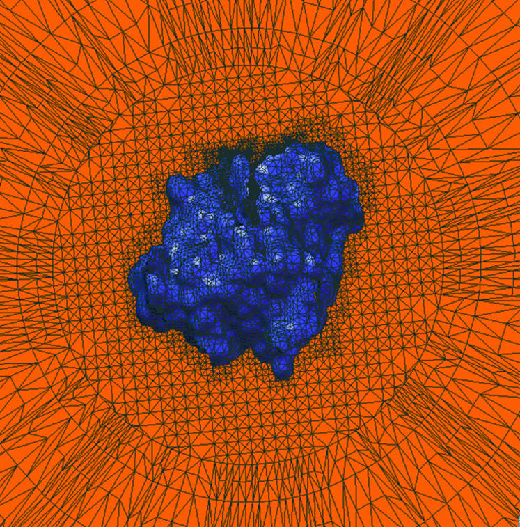
Cross section of the initial finite element mesh used for mAChE calculations.
The outer boundary of the domain was assigned bulk Dirichlet boundary conditions (Eq. 2), the nonreactive portions of the inner boundary were assigned reflective Neumann conditions (Eq. 5), and the reactive portions were assigned the “infinite reactivity” Dirichlet condition (Eq. 4). This reactive condition was chosen to agree with previous BD (Tara et al., 1998) and SE (Song et al., 2003) simulations and is justified by the extremely high catalytic efficiency of mAChE (Anglister et al., 1995). In the previous finite element SE studies, the reactive boundary was defined as the spherical reactive surface typical for Brownian dynamics calculations (Song et al., 2003). In the current study, the reactive boundary is defined using the biomolecular surface. Following Tara et al. (1998), the mAChE structure was reoriented to center the carbonyl carbon of the active site S203 at the origin and to align the active site gorge with the y axis. Reactive boundaries were based on 6 spheres placed along the y axis: sphere 1 centered at (0.0, 16.6, 0.0) with a 12 Å radius, sphere 2 centered at (0.0, 13.6, 0.0) with a 9 Å radius, sphere 3 centered at (0.0, 10.6, 0.0) with a 6 Å radius, sphere 4 centered at (0.0, 7.6, 0.0) with a 6 Å radius, sphere 5 centered at (0.0, 4.6, 0.0) with a 6 Å radius, and sphere 6 centered at (0.0, 1.6, 0.0) with a 6 Å radius. For the biomolecular surface-based reaction criteria, each reactive surface N was defined as that portion of the mAChE molecular surface inside the union of spheres N through 6. For example, surface 1 was the portion of the mAChE surface inside the union of spheres 1–6 whereas surface 6 was the portion of the mAChE surface inside 6. The six reactive surfaces defined in this manner are shown in Fig. 3 a. This definition differs considerably from the spherical reaction criteria used in the previous work (Song et al., 2003) wherein each reactive surface N was defined by explicitly including the union of spheres N−6 in the mAChE structure. For comparison, the first reactive surface of based on the spherical definition is shown in Fig. 3 b.
FIGURE 3.

Reactive boundary definitions for mAChE: (a) molecular reactive boundaries Nos. 1–6 (left to right) and (b) spherical reactive boundary No. 1.
Wild-type mAChE reaction rates
mAChE reaction rates were calculated with the initial mesh and new reactive boundary definitions described. The diffusing ligand was treated as a sphere with a +1 e charge, a 2.0 Å exclusion radius, a diffusion constant of 7.8 × 10⁴ Å2/μs; this spherical model and its parameters are similar to those used in previous BD models of the TFK+ ligand (Tara et al., 1998). Following standard procedure in BD-based rate constant calculations, only electrostatic contributions to the PMF for the SE were included in these calculations, reflecting the known importance of electrostatics in mAChE binding kinetics (Radic et al., 1997). Although the true PMF is certainly more complex than this simple description, such simple interaction models have successfully been used in numerous BD calculations of binding rate constants (for examples, see Allison and McCammon, 1985; Antosiewicz and McCammon, 1995; Tara et al., 1998). (For an excellent example of diffusion simulations with more detailed PMFs, see Im and Roux, 2002). Other considerations in developing more accurate effective ligand-protein interactions are presented in the context of protein-protein encounter simulations by Elcock et al. (2001). Finally, Roux and Simonson (1999) provide a very good general discussion of the caveats associated with the simple implicit solvent electrostatic PMF used here.
The electrostatic potential used for our PMF was obtained from the Poisson-Boltzmann equation using the APBS software (http://agave.wustl.edu/apbs/) (Baker et al., 2001b). The CHARMM22 force field was used to assign the partial changes and radii of the atoms for mAChE, the dielectric values of 4 and 78 were assigned for the protein and solvent, a solvent probe radius is 1.4 Å, and an ion exclusion layer is 2.0 Å. Various ionic strengths (between 0 and 0.670 M) were used in the PMF calculations.
Additionally, the adaptive finite element methods described above were used to calculate the reaction rates for both the molecular-surface-based (Fig. 3 a) and spherical (Fig. 3 b) reactive boundary No. 1 as a function of ionic strength. Iterative error-based refinement of the initial 656,823-simplex mesh was performed until the global error was <107, a problem-value chosen to provide reaction rates which did not change appreciably upon further refinement (see Fig. 4). The reaction rate results from these calculations are shown in Fig. 5. As this figure illustrates, the spherical and molecular-surface-based reaction criteria both give results that are in good overall agreement with each other and experiment. The comparison (at 150 mM ionic strength) between the molecular and spherical boundary definitions for the 6 reactive surfaces is shown in Fig. 6. Again, the two methods are in good overall agreement but do show some differences at surfaces No. 1 and No. 2 where the differences between the reactive boundaries—in particular, their surface areas—are most extreme (see Fig. 3).
FIGURE 4.

Percent change in the calculated wild-type mAChE reaction rates during adaptive refinement for 0 (•), 50 (▪), 100 (♦), 150 (▴), 300 (◂), 450 (×), and 670 (*) mM ionic strengths.
FIGURE 5.

Comparison mAChE wild-type ligand binding rates calculated with various methods: adaptive calculation with molecular reactive boundary No. 1 (•), nonadaptive calculation with molecular reactive boundary No. 1 (○), adaptive calculation with spherical reactive boundary No. 1 (▴), Brownian dynamics calculation with spherical reactive boundary No. 1 (▪), and from Debye-Hückel fit to experimental data (Tara et al., 1998) (solid line).
FIGURE 6.

Comparison of the mAChE wild-type binding rate results (150 mM ionic strength) as a function of reactive boundary location: (•) molecular reactive boundary and (▴) spherical reactive boundary.
Table 1 illustrates the rate constants for various ionic strengths obtained with and without error-based adaptation of the mesh. The reaction rates calculated from the adaptive finite element solution for wild-type mAChE deviate by ∼10–100% from the nonadapted calculation for the molecular reactive surface and by ∼1–10% for the spherical reactive surface. Therefore, although the mesh used in the previous work (Song et al., 2003) is fine enough for the qualitative description of ionic strength dependence, there are cases where substantial improvement is provided by the adaptive method. Furthermore, it is important to note that the simple geometric definitions used to generate the initial nonadapted mesh for mAChE may not always give even a qualitative level of predictive power without subsequent error-based refinement. In particular, molecules with high charge densities (nucleic acids, actin, etc.) will likely require error-based adaptive refinement to generate reliable diffusion profiles and rate constants. Therefore, when applying this method, it is recommended that users examine the sensitivity of the results to adaptive refinement before using rates from any nonadapted calculations.
TABLE 1.
Nonadaptive and adaptive solution results of reaction rates (in units of 109 M−1 min−1) for reactive surface 1 of wild-type mAChE
| Ionic Strength | Nonadapted results | Adapted results |
|---|---|---|
| 0 | 758 (971) | 853 (1040) |
| 50 | 249 (324) | 293 (354) |
| 100 | 209 (277) | 237 (294) |
| 150 | 188 (254) | 213 (265) |
| 300 | 152 (223) | 165 (227) |
| 450 | 117 (208) | 131 (207) |
| 670 | 35 (191) | 77 (189) |
Values not in parentheses are from the molecular reactive surface; results in parentheses are from the spherical reactive surface.
As with the spherical case, adaptive finite element calculations are significantly more expensive than their nonadapted counterparts. As for the sphere test case, the following timing data was obtained using a version of SMOL compiled with Intel FORTRAN and C (version 8.0, “−O2” optimization) and running on a 2.4 GHz Intel Xeon machine with 1.5 GB RAM. For the molecular reactive boundary, the average nonadapted runtime was 415 seconds and the average adapted runtime was 8800 seconds; for the spherical reactive boundaries the average nonadapted and adapted runtimes were 415 and 6600 seconds, respectively. The impact of this increased computational effort is discussed in the Conclusions section of this work.
Reaction rate calculation for mutant mAChE with a molecular-surface reactive boundary
One of the distinct advantages of the biomolecular reactive surface definition is the ability to directly map molecular information about the protein onto the reaction criteria. In this work, we demonstrate the ability of the biomolecular surface reactive boundary definition to correctly describe the kinetics of mAChE active site and gorge mutants. Specifically, we examined the effects of E202Q, D74N, and D74N/E202Q mutations on the mAChE ligand binding rate. The location of D74 and E202 are indicated in Fig. 3 a. D74 is located between reactive surface 3 and 4, whereas E202 is located within reactive surface 6, close to the active site. The chosen mutations constitute changes adjacent to the catalytic triad (E202Q) and in the active site gorge (D74N). These mutants have been characterized both experimentally (Radic et al., 1997) and computationally (Tara et al., 1999), using BD methods. The purpose of this work is to determine the ability of the molecular reactive surface boundary to quantitatively capture the effects of these mutations on the reaction rate.
The simulation protocol for these mutations is the same as for the ionic strength calculations described above, with one important difference. New electrostatic PMFs are recalculated for each of the three mutants at 150 mM ionic strength. Due to the isosteric nature of the mutations, all other parameters (particularly the mesh) remain unchanged.
To compare the continuum diffusion rate constants with BD results, simulations similar to those of Tara et al. (1998) were repeated using the UHBD software (Madura et al., 1995) to calculate the 150 mM ionic strength reaction rates at each of the 6 reactive surfaces for D74N, E202Q, and D74N/E202Q mutations. In particular, for each set of conditions, 5 BD runs of 200 trajectories each were simulated. The ligand was modeled as a sphere with +1 charge and a 2.0 Å radius. Each trajectory was started at a random location on a spherical surface of 55 Å (centered on the protein) and terminated when the ligand either passed the reactive boundary (see above) or a second spherical surface of radius 300 Å. The BD equation of motion was integrated using the standard Ermak-McCammon algorithm (Ermak and McCammon, 1978) and variable time steps: 5 fs at 100 Å from the mAChE center, 1 ps at 100–175 Å from the mAChE center, and 5 ps at 175–300 Å from the mAChE center.
Fig. 7 presents the log-ratios of reaction rates for the wild-type, E202Q, D74N, and D74N/E202Q mAChE calculated from the adaptive SE calculations and BD simulations at 150 mM ionic strength. This figure also includes experimental values (Radic et al., 1997) for reference. These results indicate that the continuum SE calculations generate rates with similar trends as BD; however, the actual values can differ by as much as two orders of magnitude between the two methods. Such discrepancies in predicted rates are not too surprising and simply reflect differences in methods, particularly their definitions of reactions and reactive boundaries.
FIGURE 7.

Log-ratio of reaction rates  for mAChE mutants (150 mM ionic strength) as a function of the molecular reactive boundary location. (a) D74N results: experimental (solid line), adaptive SMOL (•), and BD (▪). (b) E202Q results: (solid line), adaptive SMOL (•), and BD (▪). (c) D74N/E202Q results: experimental (solid line), adaptive SMOL (•), and BD (▪).
Fig. 7 also shows that reactive surface No. 5 provides the best overall results for the binding rate across all versions of mAChE studied. This surface is shown as the fifth picture of Fig. 3 a, which is the molecular surface along the reactive gorge within 10.6 Å from the active site. This surface is below the location of D74 but above the active site and residue E202. The agreement with experimental data and correlation with BD trends demonstrates the ability of this new adaptive method to calculate reaction rates for ligand binding both with traditional spherical and with new molecular-surface-based reactive boundaries.
CONCLUSIONS AND DISCUSSIONS
We have presented an adaptive version of the finite element solver described in an earlier work (Song et al., 2003) and demonstrated that error-based refinement of the mesh improves the calculation of reaction rates. Additionally, we have described a new molecular-surface reactive boundary definition for the SE and applied this definition to the calculation of ligand-binding rates for mAChE. The molecular-surface reactive boundary condition showed good agreement with the experimental dependence of binding rate on ionic strength and mutations. Additionally, the adaptive molecular-surface calculation results were comparable to the trends observed in BD simulations, although specific values varied by as much as two orders of magnitude between the two methods. Comparisons with experimental mutation results show that molecular reactive surface within 10.6 Å from the active site best represents the effect of D74N, E202Q, and D74N/E202Q mutations on the reaction rate of mAChE.
The timing information provided for the adaptive method illustrates that it is definitely more computationally-demanding than the nonadaptive calculations and, in some cases, even more expensive than the traditional BD simulations. However, judicious use of these expensive calculations can save substantial time and still provide an overall gain over BD simulations. As mentioned earlier, the initial mesh is generated based on the biomolecular geometry and does not necessarily provide the best possible basis set for solution of the SE. Therefore, adaptive refinement should be a standard part of finite element SE calculations to ensure the most accurate results. In particular, a “benchmark” adaptive refinement calculation is needed for each system studied to determine the error in rates calculated on the initial mesh and to obtain the global error tolerance at which the calculated rates are converged (cf. Fig. 4). However, much of the refinement performed in the each of the various adaptive calculations described above is redundant; i.e., the same regions of the initial mesh are refined for each system. Therefore, substantial time could be saved by reusing the refined mesh from the benchmark calculation as a starting point for subsequent simulations and thereby avoiding some of the expensive refinement steps.
Furthermore, as mentioned in the previous work, these continuum diffusion methods are designed to address a different scale of simulation from traditional BD methods; specifically, laying the groundwork for integration of molecular-scale information into cellular-scale systems (Smart and McCammon, 1998; Tai et al., 2003). In particular, this ability of FE-based continuum methods to integrate scales is demonstrated by performing the diffusion calculations on a finite element mesh of 0.31 μm × 0.28 μm × 0.37 μm, or ∼5 times the length of the BD domain (600 Å long). The adaptive methods developed in this work further facilitate our ultimate goal of multiscale modeling by enabling the efficient solution of the SE through adaptively allocating the unknowns based on error estimates.
Finally, one particularly useful aspect of the molecular surface boundary definition introduced in this work is the ability to directly connect the reactive surfaces of the simulation with the underlying biomolecule. For example, surface 6 maps directly onto the catalytic triad and are the most intuitive reactive boundary definitions available for this system. Additionally, these surfaces performed well in quantifying the impact of mutation on binding-rate constants. Such molecular-based reactive definitions suggest future possibilities of connecting coarse-grained simulations of diffusion with more detailed descriptions of enzyme function; in particular molecular dynamics and quantum mechanics worked describing the details of biomolecular binding and catalysis (Luty et al., 1993; Zhang et al., 2002).
Acknowledgments
N. A. Baker and C. L. Bajaj thank M. Holst for access to the FEtk software, S. Bond for help with various aspects of FEtk, and J. Andrew McCammon for access to the mAChE BD data, advice, and stimulating discussions. Y. Song thanks M. Bradley and T. Dolinsky for their help with the project.
The work at Washington University was supported by the National Science Foundation-National Partnership for Advanced Computational Infrastructure, National Biomedical Computation Resource (National Institutes of Health P41 RR08605), and an Alfred P. Sloan Research Fellowship to N.A.B. The work at the University of Texas was supported in part by National Science Foundation grants ACI-0220037, CCR-9988357, and EIA-0325550; a University of Texas-M. D. Anderson Cancer Center Whitaker grant; and a subcontract from the University of California, San Diego 1018140 as part of the National Science Foundation-National Partnership for Advanced Computational Infrastructure project.
References
- Agmon, N., and A. L. Edelstein. 1997. Collective binding properties of receptor arrays. Biophys. J. 72:1582–1594. [DOI] [PMC free article] [PubMed] [Google Scholar]
- Allison, S. A., and J. A. McCammon. 1985. Dynamics of substrate binding to copper zinc superoxide dismutase. J. Phys. Chem. 89:1072–1074. [Google Scholar]
- Anglister, L., J. R. Stiles, B. Haesaert, J. Eichler, and M. M. Salpeter. 1995. Acetylcholinesterase at neuromuscular junctions. In Enzymes of the Cholinesterase Family. D. M. Quinn, A. S. Balasubramanian, and B. P. Doctor, editors. Plenum Press, New York.
- Antosiewicz, J., and J. A. McCammon. 1995. Electrostatic and hydrodynamic orientational steering effects in enzyme-substrate association. Biophys. J. 69:57–65. [DOI] [PMC free article] [PubMed] [Google Scholar]
- Antosiewicz, J., J. A. McCammon, S. T. Wlodek, and M. K. Gilson. 1995. Simulation of charge-mutant acetylcholinesterases. Biochemistry. 34:4211–4219. [DOI] [PubMed] [Google Scholar]
- Antosiewicz, J., S. T. Wlodek, and J. A. McCammon. 1996. Acetylcholinesterase—role of the enzyme's charge distribution in steering charged ligands toward the active site. Biopolymers. 39:85–94. [DOI] [PubMed] [Google Scholar]
- Axelsson, O., and V. A. Barker. 1984. Finite Element Solution of Boundary Value Problems. Theory and Computation. Academic Press, San Diego.
- Baker, N., M. Holst, and F. Wang. 2000. Adaptive multilevel finite element solution of the Poisson-Boltzmann equation II. Refinement at solvent-accessible surfaces in biomolecular systems. J. Comput. Chem. 21:1343–1352. [Google Scholar]
- Baker, N. A., D. Sept, M. J. Holst, and J. A. McCammon. 2001a. The adaptive multilevel finite element solution of the Poisson-Boltzmann equation on massively parallel computers. IBM J. Res. Dev. 45:427–438. [Google Scholar]
- Baker, N. A., D. Sept, S. Joseph, M. J. Holst, and J. A. McCammon. 2001b. Electrostatics of nanosystems: Application to microtubules and the ribosome. Proc. Natl. Acad. Sci. USA. 98:10037–10041. [DOI] [PMC free article] [PubMed] [Google Scholar]
- Braess, D. 1997. Finite Elements. Theory, Fast Solvers, and Applications in Solid Mechanics. Cambridge University Press, Cambridge.
- Elcock, A. H., M. J. Potter, D. A. Matthews, D. R. Knighton, and J. A. McCammon. 1996. Electrostatic channeling in the bifunctional enzyme dihydrofolate reductase-thymidylate synthase. J. Mol. Biol. 262:370–374. [DOI] [PubMed] [Google Scholar]
- Elcock, A. H., D. Sept, and J. A. McCammon. 2001. Computer simulation of protein-protein interactions. J. Phys. Chem. B. 105:1504–1518. [Google Scholar]
- Ermak, D. L., and J. A. McCammon. 1978. Brownian dynamics with hydrodynamic interactions. J. Chem. Phys. 69:1352–1360. [Google Scholar]
- Gabdoulline, R. R., and R. C. Wade. 1998. Brownian dynamics simulation of protein-protein diffusional encounter. Methods 14:329–341. [DOI] [PubMed] [Google Scholar]
- Holst, M. 2001. Adaptive numerical treatment of elliptic systems on manifolds. Adv. Comp. Math. 15:139–191. [Google Scholar]
- Holst, M., N. Baker, and F. Wang. 2000. Adaptive multilevel finite element solution of the Poisson-Boltzmann equation I. Algorithms and examples. J. Comput. Chem. 21:1319–1342. [Google Scholar]
- Im, W., and B. Roux. 2002. Ion permeation and selectivity of OmpF porin: a theoretical study based on molecular dynamics, Brownian dynamics, and continuum electrodiffusion theory. J. Mol. Biol. 322:851–869. [DOI] [PubMed] [Google Scholar]
- Krissinel, E. B., and N. Agmon. 1996. Spherical symmetric diffusion problem. J. Comput. Chem. 17:1085–1098. [Google Scholar]
- Kurnikova, M. G., R. D. Coalson, P. Graf, and A. Nitzan. 1999. A lattice relaxation algorithm for three-dimensional Poisson-Nernst-Planck theory with application to ion transport through the gramicidin A channel. Biophys. J. 76:642–656. [DOI] [PMC free article] [PubMed] [Google Scholar]
- Luty, B. A., S. Elamrani, and J. A. McCammon. 1993. Simulation of the bimolecular reaction between superoxide and superoxide dismutase: synthesis of the encounter and reaction steps. J. Am. Chem. Soc. 115:11874–11877. [Google Scholar]
- Madura, J. D., J. M. Briggs, R. C. Wade, M. E. Davis, B. A. Luty, A. Ilin, J. Antosiewicz, M. K. Gilson, B. Bagheri, L. R. Scott, et al. 1995. Electrostatics and diffusion of molecules in solution—simulations with the University of Houston Brownian Dynamics Program. Comput. Phys. Commun. 91:57–95. [Google Scholar]
- Northrup, S. H., S. A. Allison, and J. A. McCammon. 1984. Brownian dynamics simulation of diffusion-influenced biomolecular reactions. J. Chem. Phys. 80:1517–1524. [Google Scholar]
- Radic, Z., P. D. Kirchhoff, D. M. Quinn, J. A. McCammon, and P. Taylor. 1997. Electrostatic influence on the kinetics of ligand binding to acetylcholinesterase—distinctions between active center ligands and fasciculin. J. Biol. Chem. 272:23265–23277. [DOI] [PubMed] [Google Scholar]
- Roux, B., and T. Simonson. 1999. Implicit solvent models. Biophys. Chem. 78:1–20. [DOI] [PubMed] [Google Scholar]
- Schuss, Z., B. Nadler, and R. S. Eisenberg. 2001. Derivation of Poisson and Nernst-Planck equations in a bath and channel from a molecular model. Phys. Rev. E. 64:036116. [DOI] [PubMed] [Google Scholar]
- Smart, J. L., and J. A. McCammon. 1998. Analysis of synaptic transmission in the neuromuscular junction using a continuum finite element model. Biophys. J. 75:1679–1688. [DOI] [PMC free article] [PubMed] [Google Scholar]
- Song, Y., Y. Zhang, T. Shen, C. L. Bajaj, J. A. McCammon, and N. A. Baker. 2003. Finite element solution of the steady-state Smoluchowksi equation for rate constant calculations. Biophys. J. 86:2017–2029. [DOI] [PMC free article] [PubMed] [Google Scholar]
- Stiles, J. R., and T. M. Bartol. 2000. Monte Carlo methods for simulating realistic synaptic micro-physiology using MCell. In Computational Neuroscience: Realistic Modeling for Experimentalists. E. De Schutter, editor. CRC Press, New York.
- Tai, K., S. D. Bond, H. R. MacMillan, N. A. Baker, M. J. Holst, and J. A. McCammon. 2003. Finite element simulations of acetylcholine diffusion in neuromuscular junctions. Biophys. J. 84:2234–2241. [DOI] [PMC free article] [PubMed] [Google Scholar]
- Tara, S., A. H. Elcock, P. D. Kirchhoff, J. M. Briggs, Z. Radic, P. Taylor, and J. A. McCammon. 1998. Rapid binding of a cationic active site inhibitor to wild type and mutant mouse acetylcholinesterase: Brownian dynamics simulation including diffusion in the active site gorge. Biopolymers. 46:465–474. [DOI] [PubMed] [Google Scholar]
- Tara, S., T. P. Straatsma, and J. A. McCammon. 1999. Mouse acetylcholinesterase unliganded and in complex with huperzine A: a comparison of molecular dynamics simulations. Biopolymers. 50:35–43. [DOI] [PubMed] [Google Scholar]
- Zhang, Y., C. Bajaj, and B. S. Sohn. 2003. Adaptive and Quality 3-D Meshing from Imaging Data. Proc. ACM SM 2003. ACM Press, Seattle. 286–291. (Full version to appear in CMAME).
- Zhang, Y., J. Kua, and J. A. McCammon. 2002. Role of the catalytic triad and oxyanion hole in acetylcholinesterase catalysis: An ab initio QM/MM study. J. Am. Chem. Soc. 124:10572–10577. [DOI] [PubMed] [Google Scholar]