Model-Based Fitting of Single-Channel Dwell-Time Distributions

Abstract

Single-channel recordings provide unprecedented resolutions on kinetics of conformational changes of ion channels. Several approaches exist for analysis of the data, including the dwell-time histogram fittings and the full maximal-likelihood approaches that fit either the idealized dwell-time sequence or more ambitiously the noisy data directly using hidden Markov modeling. Although the full maximum likelihood approaches are statistically advantageous, they can be time-consuming especially for large datasets and/or complex models. We present here an alternative approach for model-based fitting of one-dimensional and two-dimensional dwell-time histograms. To improve performance, we derived analytical expressions for the derivatives of one-dimensional and two-dimensional dwell-time distribution functions and employed the gradient-based variable metric method for fast search of optimal rate constants in a model. The algorithm also has the ability to allow for a first-order correction for the effects of missed events, global fitting across different experimental conditions, and imposition of typical constraints on rate constants including microscopic reversibility. Numerical examples are presented to illustrate the performance of the algorithm, and comparisons with the full maximum likelihood fitting are discussed.

INTRODUCTION

The conformational changes of proteins are often modeled as a Markov process, where the transitions between conformations are independent of history, but only on the current state. As such, the data can be analyzed via Markov modeling to probe the information about the underlying mechanisms. The best-studied examples are the molecules of ion channels, where single-channel recording, consisting of a sequence of dwell-times at different conductance levels, provides a detailed view on the time course of the dynamics of the channel protein.

Several approaches exist for analysis of single-channel data. The simplest, but perhaps the most common one, is the fitting of duration histograms. The Markov theory predicts that the distributions of the dwell-times of a subset of states, e.g., the closed or the open states, follow sums of exponential functions. Therefore, fitting the histograms of open or closed dwell-times can provide information on some aspects of the underlying process, such as the minimal number of states, the time constants, and proportions of the individual components. The one-dimensional histograms do not contain correlations between adjacent events, which is only available in the high-order distributions (Fredkin et al., 1985) and is crucial for identification of models with complex topologies (Rothberg and Magleby, 1998). The use of time constants also incurs the difficulty to allow for simultaneous fitting of multiple distributions across different conditions. Such problems can be alleviated by fitting two-dimensional dwell-time distributions with explicit kinetic schemes (Rothberg and Magleby, 1998).

More advanced techniques include the maximum likelihood fitting of dwell-time sequences, the hidden Markov modeling (HMM), and the simulation-based approach. The dwell-time sequence approach calculates the distribution of entire dwell-time sequences and optimizes the model so as to maximize the probability (Horn and Lange, 1983; Ball and Sansom, 1989; Qin et al., 1997, 1996; Colquhoun et al., 1996, 2003). Procedures for rapid evaluation of likelihood function and its derivatives have been developed, which allow fast search for the maximum likelihood (Qin et al., 1997). Essential to the success of the approach is the correction for missed events. Due to limited-time resolution, brief events may go undetected, and as a result, the apparent dwell-time durations become elongated. Such distortions are generally taken into account by appropriately correcting the dwell-time distributions predicted from the model assuming a fixed dead time. Both exact and approximate solutions to the problem have been developed (Blatz and Magleby, 1986; Roux and Sauve, 1985; Crouzy and Sigworth, 1990; Hawkes et al., 1990, 1992; Colquhoun et al., 1996). With a first-order correction, the full likelihood approach has been shown to work reasonably well for a variety of channels while maintaining the feasibility for analytical evaluations of the derivatives of the likelihood function (Qin et al., 1996).

Hidden Markov modeling is also a full maximum likelihood approach, but it differs from the dwell-time sequence fitting in that it fits a model to the samples. The model has two parts; one is the kinetics of the channel, and the other the current amplitudes and noise statistics. The general theory of HMM has been applied to many problems including speech recognition, gene finding, sequence alignment, and so on. Its application to molecular kinetic modeling imposes some novel challenges, such as the parameterization of rate constants, the dependence of parameters on experimental conditions, and the characteristic non-white noise. Several approaches have been proposed to tackle these problems (Venkataramanan and Sigworth, 2002; Qin et al., 2000a,b). Because noise is taken into explicit account, the HMM has the advantage of eliminating the need of intermediate idealizations of raw data. The expense of doing so, however, is the significantly increased computational load, since the probability of the model has to be evaluated through individual samples instead of dwell-times.

The simulation-based approach exploits a different paradigm based on iterative simulations of single-channel currents and comparisons of the resulting dwell-time histograms with the experimental ones (Magleby and Weiss, 1990a,b). The simulated currents are analyzed in a manner identical to that used to analyze the experimental data, so that the resulting dwell-time histograms are subject to the same distortions that occur on the experimental ones. As a result, problems like low-pass filtering and missed events are taken account of implicitly. Unfortunately, the approach is computationally inefficient because of the need to repeatedly simulate and idealize the data.

The maximum likelihood fitting of dwell-time sequences is more efficient than the HMM and the simulation approach, and proves adequate for many problems. However, it has a computational complexity that increases more than quadratically with the size of the model and linearly with the number of events (Qin et al., 1996). For large models and/or long data sets, the approach can be prohibitively slow, taking hours to days. This is the case, for example, when the gating of the channel involves multiple subunits, and transitions within a subunit consist of multiple steps. Problems like this can easily result in models with tens of states. For such problems, histogram fitting becomes a handy alternative, especially when limited computational resources are available.

We present here an improved procedure for histogram fitting. The approach uses iterative fitting of one-dimensional and two-dimensional dwell-time distributions to estimate rate constants, as has been done previously. We have greatly speeded up the method with a derivative search for the rate constants and compared the method to the full likelihood method, where it is found to compare favorably in estimating rate constants, but is much faster for large amounts of data. Finally, the fitting programs are made available through the QuB site.

THEORY

Dwell-time distributions

The gating of the channel is modeled as a stochastic Markov process, x(t), with a finite state space {s_i, i = 1…N}. The transitions between states are described by the first-order rate constants k_ij, i.e.,

(1)

For ion channels, the transitions are observed as discrete jumps between conductance levels. There may be multiple states with the same conductance, and the transitions among such states are not observed directly. Instead, they can only be deduced from statistical distributions.

For convenience of notation, the rate constants are collectively designated by a matrix Q = [k_ij]_N×N, which is known as the infinitesimal generator matrix (Colquhoun and Hawkes, 1982). The (i,j)^th element of the matrix defines the rate from state i to state j, and the diagonal elements are defined so that the sum of each row equals to zero, for the conservation of flux through state i. According to the observable classes, the matrix is partitioned so that the states of the same class are adjacent to each other, i.e.,

where the diagonal blocks designate rates of transitions within the classes and the off-diagonal ones between classes.

The discrete jumps observed between different conductance levels can be described by two essential probabilities. One is the probability of transitions between states within a class, and the other the probability to leave for another class. They can be formulated respectively (Colquhoun and Hawkes, 1982) as

(2)

(3)

where the (i,j)^th element of P_aa(t) is the probability to start from state i and end at state j after time t without leaving the class, and similarly, the (i,j)^th element of P_ab(Δt) is the probability of a transition from state i of class a to state j of class b in an infinitesimal time Δt.

Given the probabilities for transitions within a class and between two classes, the distribution of an observed dwell-time at a given conductance level follows (Colquhoun and Hawkes, 1982) as

(3a)

where π_a specifies the probability of the channel to enter the states of class a at the equilibrium, represents the set of the complement states not in class a, and summarizes the probability of transitions leaving class a for an unknown destination state. That is, the distribution is given by the entry probability into the class, multiplied by the probability of transitions within the class, and then the probability to exit the class.

The entry probability π_a is given by (Fredkin et al., 1985)

(4)

which defines a set of homogeneous equations, and can be solved in combination with the probability totality constraint.

Similarly, the two-dimensional dwell-time distributions, i.e., the joint probability of two adjacent dwell-times of different classes, are given by (Fredkin et al., 1985)

(5)

that is, the probability entering the first class, multiplied by the probability of transitions between states within that class, multiplied by the probability of transitions from states in the first class to states in the second class, and so on.

In general, the higher the order of a distribution, the more information it contains. However, there is an upper limit on the maximal order it needs before having all the information of the data. The limit depends on the number of observable classes. For a process with two classes at equilibriums, there is an elegant theory stating that the third-order distributions do not contain more information than those of the second-order (Fredkin et al., 1985). In the other words, the distributions with orders higher than two are redundant, and they can be obtained from the one-dimensional and two-dimensional distributions. Ion channels are mostly binary, either closed or open. The theory implies that the two-dimensional dwell-time distributions provide a complete information context, and therefore suffice to describe the data at equilibriums. For this reason, we will restrict ourselves in the following to the case of binary channels.

For binary channels, the distributions described above can be simplified. Following the conventional notation with C and O representing the two classes, the dwell-time distributions can be rewritten as

(6)

(7)

(8)

(9)

and the entry probability as

(10)

(11)

where Q_cc corresponds to the transitions between closed states, Q_co from closed states to open states, Q_oc from open states to closed states, and Q_oo between open states.

Evaluation of dwell-time distributions

Given a set of rate constants, the dwell-time distributions can be evaluated using standard matrix decomposition techniques as previously described (Qin et al., 1997). Briefly, from the eigenvalues and eigenvectors of a rate matrix, one can determine the corresponding transition probability matrix as

(12)

(13)

where n_a is the number of states in class a, λ_i-values are the eigenvalues of Q_aa, and A_i values are the matrices multiplied from the eigenvectors (Colquhoun and Hawkes, 1982). The one-dimensional and two-dimensional dwell-time distributions are then given by

(14)

(15)

and

(16)

(17)

respectively, where for simplicity of notation the closed and open eigenvalues are designated differently with λ- and μ-values, respectively. The entry probability is determined by the linear equation

where the matrix Φ_aa can be reformulated into

(18)

(19)

These equations allow the matrix to be evaluated analytically from the expansions of Q_cc and Q_oo without the need to calculate their inversions. The dwell-time distribution equations suggest that the one-dimensional distributions have the form of sums of one-dimensional exponentials whereas the two-dimensional distributions are sums of two-dimensional exponentials.

Derivatives of dwell-time distributions

The availability of the derivatives of the dwell-time distribution functions is essential to rapid optimization of likelihood function as well as to accurate estimation of model parameters. The calculation of the derivatives involves several steps. But the central step is the calculation of the derivatives of a matrix exponential, which follows

(20)

where γ is a scalar function determined by the eigenvalues (Ball and Sansom, 1989; Qin et al., 1996). From the equation, the derivatives of the one-dimensional dwell-time distributions can be obtained as

(21)

and the two-dimensional dwell-time distributions as

(22)

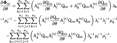
For the derivatives of the entry probability, one first calculates the derivatives of the matrix Φ_cc, which can be derived as.

(23)

The derivatives of the entry probability are then determined by

(24)

The equation has the same coefficient matrix as the one for the entry probability itself; therefore they can be solved together to reduce computations. Note that only the derivatives of the closed distribution f_c(t) and the closed and open distribution f_co(t,s) are described here; the derivations of the other two distributions, the open distribution f_o(s) and the open and closed distribution f_oc(s,t), are in exact parallels.

Likelihood functions

The goodness of a fit is ranked using the pseudo-likelihood criterion as for exponential-based histogram fitting (Colquhoun and Sigworth, 1995). The likelihood of a one-dimensional fit is defined as

(25)

where F-values are the probabilities of dwell-times with durations in the range of specified bins. Similarly, the likelihood of a two-dimensional fit is given as

(26)

where F-values are the joint probabilities of the pairs of closed-and-open or open-and-closed dwell-times. For fine bins of small durations, the probabilities are approximately proportional to the density functions. For large bins, they are calculated by integrating the corresponding density functions over the bins. Since the distributions are of sums of exponentials, the integrals can be readily calculated by Eqs. 14–17. The small bins can provide statistically efficient estimates, but they may incur the problem of intensive computations.

In practice, the likelihoods themselves may be out of computer numeric ranges. To avoid possible overflow, the log likelihoods are used instead, yielding

(27)

(28)

The derivatives of the log likelihoods can be written as

(29)

(30)

where the derivatives of the probability F values in the summations can be obtained analytically from the derivatives of the dwell-time distribution functions in Eqs. 21 and 22.

Note that the likelihood functions defined above involve multiple distributions. For one-dimensional, the likelihood consists of both closed and open dwell-time distributions, and for two-dimensional, it involves both closed-open and open-closed dwell-time distributions. This is different from the exponential-based histogram fitting where each individual histogram is fitted separately. For model-based fitting, the distributions are not independent and need to be fitted simultaneously. Furthermore, for global fitting of data spanning over a range of experimental conditions, the likelihoods can be further extended to sum over all distributions across different individual conditions.

Maximization of likelihood functions

Estimation of model parameters is based on maximization of the pseudo-likelihood functions for dwell-time distributions. The optimization is carried out using the same approach as proposed previously for maximizing the full likelihood of dwell-time sequences (Qin et al., 1997, 1996). Briefly, the rate constants are parameterized into

(31)

where C_ij is the concentration of the drug that the rate k_ij is sensitive to and V is the membrane potential or other global variables such as force. Instead of solving for the rate constants directly, the parameters a_ij and b_ij are chosen as variables. For the rates that are independent of concentrations, C_ij = 1. Similarly, for the rates that are independent of voltages, b_ij = 0. In the case that the data does not span over multiple conditions, it follows that k_ij = a_ij.

The above parameterization of rate constants has the advantage to allow for combined fitting of multiple distributions from different experimental conditions. A further twist in the implementation is that the variables a_ij are actually represented in their exponential forms. By doing so, it facilitates the handling of multiplicative constraints such as the detailed balance conditions. With the new representation, these constraints are reduced to linear equations, which can be taken into account explicitly by matrix decompositions.

Search of the likelihood space is performed using a quasi-Newtonian method (Press et al., 1992). The method exploits an approximate Hessian matrix accumulated from the first-order derivatives and features a quadratic convergence near the maximal point. Other optimizers were also attempted, but they were generally inferior to the quasi-Newtonian approach, particularly in terms of the accuracy of the estimates. For example, the non-gradient-based simplex method was often found to bog down when the parameters were still far away from the true values. The problem becomes increasingly aggravated when the parameter space is large.

Correction for missed events

The effects of missed events on the apparent dwell-time durations are corrected using a first-order approximation (Roux and Sauve, 1985; Qin et al., 1996). Given a fixed dead time t_d, this is done by simply correcting the rate constant matrix,

(32)

(33)

where a and b are ether closed or open, but a ≠ b, and the matrix E_aa is the correction term given by

(34)

Both the correction matrix itself and its derivatives can be calculated analytically from the spectral expansions of the rate constant matrices (Qin et al., 1996). There are other solutions, both approximate and exact, to the missed events problem (Crouzy and Sigworth, 1990; Hawkes et al., 1992). Although these solutions are more accurate (Hawkes et al., 1990), the first-order approximation has the advantage on the availability of its analytical derivatives. This is important since it allows one to use fast optimization algorithms to search the likelihood space; otherwise, one has to either evaluate the derivatives numerically or employ non-derivative-based optimizers, both of which can slow down the fitting process significantly. The first-order approximation is valid under the assumption that the missed event durations are negligible compared to the apparent durations.

Examples

A few examples are presented here to demonstrate the performance of the algorithm and its applicability to experimental data. Examples are also given to illustrate the limit of one-dimensional fitting and the improvement of two-dimensional fitting. For simulation, continuous dwell-times were generated using exponentially distributed random numbers. Histograms of dwell-time durations were constructed with logarithmically scaled binning. Probabilities of individual bins were integrated explicitly from dwell-time distributions. Calculations of eigenvalues and eigenvectors were performed using routines translated from EISPACK (www.netlib.org; see also Wilkinson and Reinsch, 1971). Several methods were implemented for search of the likelihood space, including the non-gradient-based simplex method, the gradient-based variable metric method, and the conjugate gradient method. These optimizers were taken from the book Numerical Recipes (Press et al., 1992), with modifications on step size and exception handling. The fitting was monitored with visual display of the predicted one-dimensional and two-dimensional dwell-time distributions in superimposition with experimental histograms. At the end of fitting, the time constants and proportions of individual closed and open components were calculated from the resultant model. The algorithm is implemented in C/C++ with a graphical user interface. The program is available through the IcE/QuB software suite (www.qub.buffalo.edu).

A sequential model

A linear sequential model has the simplest topology, but nevertheless has been successfully used to describe the gating of many ion channels. Scheme I shows such a model for nicotinic acetylcholine receptor (nAChR) ion channels. The model consists of two binding steps with a single open state. Table 1 (column 2) lists the values of the rate constants. For simulation, a set of 89,000 events was generated for both closed and open dwell-times, which corresponds to ∼7 min in total duration.

SCHEME I.

TABLE 1.

Parameter estimates by different approaches for Scheme I

Rate	True value	Estimate* (1D)	Estimate† (1D)	Estimate† (2D)	Estimate† (MIL)
k12	200	211	209	211	210
k21	500	516	522	532	524
k23	400	428	451	432	527
k32	25,000	27,882	28,981	29,165	34,657
k34	60,000	50,326	48,793	54,777	38,974
k43	240	196	184	202	149

^*No dead time was imposed.

^†Maximal dead times were used, with t_d = 30, 40, and 50 μs for the one-dimensional histogram fitting, the two-dimensional histogram fitting and the full likelihood fitting, respectively.

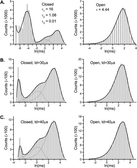
One essential feature of the model is that it has a single closed state leading to the openings. Models of this kind have no correlation between closed and open dwell-times. As a result, the one-dimensional dwell-time distributions contain sufficient information to resolve them. Table 1 (column 3) lists the estimation results for Scheme I obtained by fitting the one-dimensional dwell-time histograms. As expected, the estimates were all close to the true values of the rate constants. Fig. 1 A shows the corresponding closed and open dwell-time distributions predicted from the resultant model, which superimposed well with the histograms. It is emphasized that the model is fit to both closed and open histograms simultaneously, and the fitting resulted in rate constants directly, without relying on conversion from time constants.

FIGURE 1.

Histogram analysis of a linear sequential model. The one-dimensional histogram fitting sufficed to resolve the model (A), but it is less sustainable to missed events (B) than the two-dimensional histogram fitting (C). The imposition of a dead time had the most profound effect on the short closures (the leftmost peak in the solid histograms). The openings remained a single exponential, but the mean time increased. Data were simulated from the nicotinic ACh receptor ion channel in Scheme I. The solid lines show the overall distributions predicted from the estimated models, and the dotted lines represent the individual components.

Different dead times were attempted to assess the capability of the algorithm for correction of missed events. Although both one-dimensional and two-dimensional fittings were able to resolve the model, they appeared to have different sensitivity to missed events. For one-dimensional fitting, the algorithm worked up to a dead time t_d = 30 μs. This dead time was about the lifetime of the shortest closed state and led to a nearly 60% loss of events. For two-dimensional fitting, an even larger dead time, t_d = 40 μs, was allowed, suggesting that the two-dimensional fitting has a higher degree of tolerance for missed events. The full maximum likelihood fitting of the entire dwell-time sequence was most robust, with t_d = 50 μs. Table 1 (columns 4–6) lists the estimates from different fittings. Fig. 1, B and C, show the histograms and the distributions predicted from the best one-dimensional and two-dimensional fits with the maximally imposed dead times. As compared to the original distributions, the missed events produced considerable distortions in the closed histogram, especially on the peak of the short closures. With t_d = 50 μs, only a small tail of the peak remained. The algorithm, however, was capable of extrapolating it back to recover all the estimates. The example also illustrates that the high-order dwell-time distributions can be more reliable in practice, even though they may contain no more information than the one-dimensional distributions.

A branched model

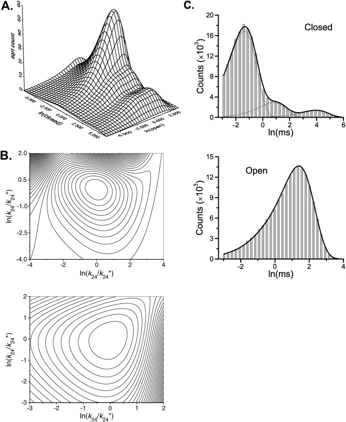
Branched models are another type of commonly used model. These models are often useful in describing channels that exhibit partial activity, e.g., openings from partial ligand binding. Scheme II illustrates an example, which was proposed for gating of Ca²⁺-activated K⁺ channels (Magleby and Pallotta, 1983). The two open states are connected to two different closed states. As a result, correlations arise between different closed and open dwell-times (Magleby and Weiss, 1990b; Magleby and Song, 1992). Fig. 2 A shows the two-dimensional dwell-time distribution predicted by the model. The rate constants used for simulation are given in Table 2, column 2. One essential feature of the distribution is that the one-dimensional sections sliced along different closed or open durations have different appearances. This is particularly evident in the open dwell-time distributions adjacent to the long and the short closures. The former exhibited two distinct peaks, whereas the latter exhibited only one. A feature like this in the two-dimensional dwell-time distributions is indicative of the existence of correlations between adjacent dwell-times.

SCHEME II.

FIGURE 2.

Models that cannot be discriminated by one-dimensional dwell-time distributions can be resolved by high-order dwell-time distributions, but they may remain as local maximum solutions. (A) The two-dimensional dwell-time distribution predicted from Scheme II for Ca²⁺-activated potassium channels. The existence of coupling between closed and open dwell-times is evident from the different appearances of the one-dimensional open dwell-time distributions in adjacency to different closed durations. (B) Contours of the likelihood surface at the true solution (top) and a local maximum point (bottom). Each interval corresponds to 918 (top) and 38,835 (bottom) log likelihood units, respectively. The local maximal solution is inferior to the true one by ∼4000 units. The axes represent the logarithms of the ratios of the rates to their true values used in simulation (top) or to their local maximum solutions (bottom). (C) The one-dimensional dwell-time distributions predicted by the local maximal solution. It fits well both closed and open histograms. The dotted lines represent the individual components. A dead time of 40 μs was used for all analysis except for the plot of the theoretical two-dimensional dwell-time distribution in A.

TABLE 2.

Parameter estimates by one-dimensional and two-dimensional dwell-time histogram fitting for Scheme II

Rate	True value (s−1)	Estimate* (1D)	Estimate† (1D)	Estimate* (2D)	Estimate† (2D)
k12	34	34	24	34	23
k21	180	181	291	180	274
k23	285	286	333	285	381
k32	600	603	332	601	388
k24	120	117	3918	117	3850
k42	2860	2770	320	2839	323
k35	3950	3926	245	3924	185
k53	322	320	2853	320	3137

^*Estimates given by one-dimensional and two-dimensional histogram fittings starting with an initial value of 100 for all rates. A dead time of t_d = 40 μs was imposed.

^†Estimates obtained with a starting value of 100 for all rates except k₂₄ = 5000, k₄₂ = 300, and k₅₃ = 2000. A dead time of t_d = 40 μs was imposed.

A linear branched model has a complexity the same as a linear sequential model, both of which involve a total of 2(N–1) rate constants, where N is the number of states. This complexity coincides with the total degrees of freedom in the one-dimensional dwell-time histograms. Therefore, it seemed that the one-dimensional histograms had sufficient complexity to resolve the model. Unfortunately, the problem is complicated by the branched openings. For the particular model in Scheme II, it has been shown that the one-dimensional histograms cannot discriminate it from other branched or sequential models (Magleby and Weiss, 1990b). Furthermore, even with a fixed topology, the fitting of one-dimensional histograms may not have a unique solution. For example, starting with all rates equal to 100 s⁻¹ for Scheme II, the one-dimensional fitting correctly estimated all parameters, as listed in Table 2, column 3. However, when perturbing the starting values to k₂₄ = 5000, k₄₂ = 300, and k₅₃ = 2000, the fitting converged to a different model (Table 2, column 4). The model, as opposed to the correct one, has the fast openings arising from C₂ and the slow ones from C₃. However, the model retained exactly the same maximum likelihood. The analysis imposed a dead time t_d = 40 μs, which resulted in a 30% loss from a total of 500,000 simulated dwell-times.

One might expect that the failure of one-dimensional histogram fitting was due to the absence of the dwell-time correlation information, and therefore could be avoided if that information was used. Unfortunately, this was only partially true. On the one hand, a high-order distribution such as the two-dimensional histograms or the full dwell-time sequence distribution did give different likelihood values for the two isomeric models obtained by the one-dimensional fitting, with the correct one scoring a higher likelihood. On the other hand, the fitting still failed when starting from the initial values that bogged down the one-dimensional fitting. This was true for both two-dimensional histogram fitting and the full maximum likelihood approach. Examination of the likelihood surface showed that the two isometric models were both the maxima of the likelihood function, even though the incorrect model has an inferior likelihood value (Fig. 2 B). Therefore, it seemed that without the use of correlation information, the two maximums attained identical likelihood values. The addition of the correlation information suppressed the likelihood value of the incorrect model, but did not suffice to remove it. As a result, it became a local maximum point. Fig. 2 C shows the one-dimensional dwell-time distributions calculated from the inferior model. As expected, it fits well both the open and the closed histograms. The presence of such local maximums certainly introduces additional complexity to the fitting, which needs to be guarded carefully against inferior local solutions.

An allosteric model

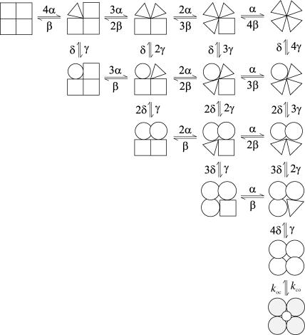
Gating of ion channels involves allosteric transitions between multiple subunits. A faithful description of the process usually requires many conformational states. Scheme III illustrates such an example. The model was modified from that proposed for gating of Shaker K⁺ channels (Zheng and Sigworth, 1997). The channel consists of four identical subunits, and each subunit involves two steps of conformational changes. The transitions between subunits are independent except the last step of opening, which is concerted.

SCHEME III.

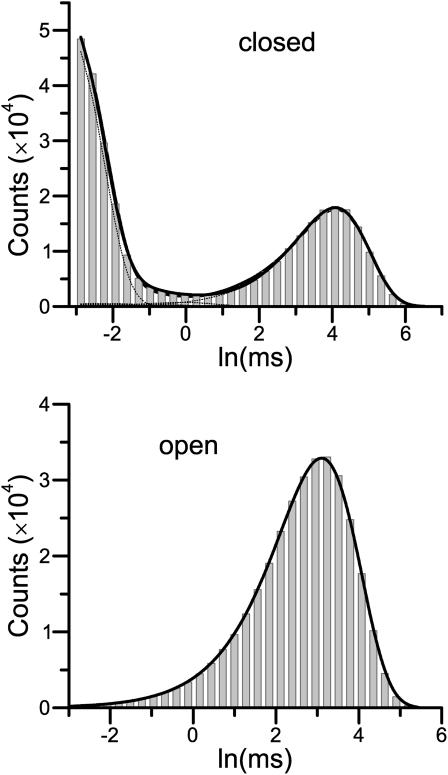
The model is large in size but involves only a few free parameters, and therefore is well suited for histogram analysis. As a test, a sequence of ∼1.2 × 10⁶ dwell-times was generated from the scheme. Table 3 (column 2) lists the values of the rate constant used in simulation. Both one-dimensional and two-dimensional histograms were fitted. A dead time t_d = 40 μs was imposed, which resulted in a loss of approximately one-half of the total number of dwell-times. Fig. 3 shows the one-dimensional histograms of the remaining dwell-times. The nature of the allosteric transitions was taken into account by imposition of constraints among the rate constants. There are a total of 36 such constraints, leaving six independent variables. The final estimates of the parameters were listed in Table 3, columns 3–4. The two-dimensional fitting successfully recovered all parameters to a good accuracy, whereas the one-dimensional fitting performed poorly on the rates between distant closed states, presumably due to the existence of branched transitions. Despite the biases on the estimated parameters, the one-dimensional fitting produced dwell-time distributions that were virtually no different from those generated by the two-dimensional fitting and fitted the histograms well, as shown in Fig. 3. The example again demonstrates the inadequacy of one-dimensional histograms for resolving branched models, even in the presence of a large number of constraints. It should be note that such ambiguity is generally pertinent to the use of a single dataset and could be reduced if the one-dimensional fitting is carried out for simultaneous fitting of data obtained under a number of experimental conditions. For this example, the two-dimensional histogram fitting took ∼1 min to converge, starting from a set of initial values at one-tenth of the true values.

TABLE 3.

Parameter estimates by one-dimensional and two-dimensional dwell-time histogram fitting for Scheme III

Parameter	True value (s−1)	Estimate (1D)	Estimate (2D)
α	1000	220	989
β	500	26	505
δ	2000	1925	2036
γ	1000	722	1023
kco	20,000	18,688	19,635
koc	100	95	97

FIGURE 3.

Dwell-time histograms and their best one-dimensional and two-dimensional fits (solid lines) for the allosteric model in Scheme III. The dotted lines superimposed on the histograms represent the individual components calculated from the two-dimensional fit. The one-dimensional and two-dimensional fits were virtually identical in the overall distributions. However, they differed in the individual closed components. Most closed components had a negligible occurrence, except the ones that constituted the two major peaks at τ = 0.038 and 52 ms, respectively.

Application to experimental data

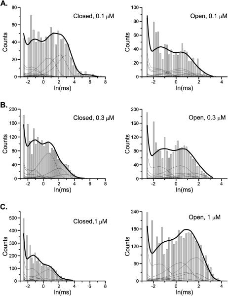
As a last example, we consider the analysis of real data from a VR1 receptor ion channel expressed in Xenopus oocytes. The recordings were made from outside-out patches perfused with different capsaicin concentrations. Data were digitized at a sampling rate of 20 kHz and lowpass-filtered to 10 kHz. Three concentrations were chosen for combined analysis. The idealization of the data was performed using the SKM procedure, with resulting dwell-times at 0.1, 0.3, and 1 μM capsaicin, respectively. A dead time of 40 μs was imposed to correct for missed events.

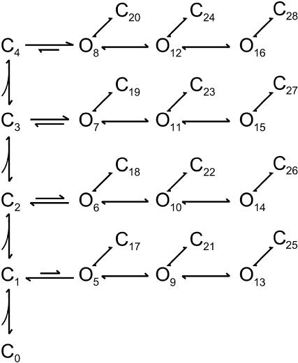
Preliminary analysis (Hui et al., 2003) suggested that the gating of the channel involves multiple closed (≥5) and open (≥3) states, and that all open states are accessible from each level of ligand binding. The open time constants are invariant to ligand concentrations, suggesting that ligand binds exclusively to the closed channel. Scheme IV illustrates a hypothesized model that is consistent with the observations. Four ligand-binding steps are assumed, with each binding leading to a burst of openings interrupted by brief closures. Multiple bindings tend to stabilize the burst, but the activity within bursts is independent of the level of ligand binding. Furthermore, it is assumed that the binding and unbinding of capsaicin to different subunits is independent.

SCHEME IV.

Fig. 4 shows the dwell-time distributions resulting from the two-dimensional histogram fit. The model involves 29 states and 56 transition rates. After taking account of all constraints, 20 independent variables remain. Table 4 lists the values of the resultant rate constants. The fitting involves six two-dimensional histograms, i.e., two closed-open and open-closed distributions at three concentrations. Also shown are the distributions of the individual closed and open components, which were calculated from the fitted model. There were eight distinct closed and twelve open components, of which only the four longest closed ones showed dependence on ligand concentration.

FIGURE 4.

Single-channel analysis of a VR1 receptor ion channel. The two-dimensional histograms constructed from three different ligand concentrations were fit simultaneously with a model showing independent ligand binding but partial openings. The solid lines superimposed on the histograms correspond to the one-dimensional dwell-time distributions predicted from the resultant model. The dotted lines represent the individual components. There were a total of 8 closed and 12 open components at each concentration, of which only four closed components exhibited concentration-dependent time constants. The other components including all openings varied in their proportions as the ligand concentration changed. A dead time of 40 μs, corresponding to two sampling durations, was imposed for the analysis.

TABLE 4.

Parameter estimates by two-dimensional dwell-time histogram fitting for Scheme IV

Rate (s−1)	Estimate (2D)	Rate (s−1)	Estimate (2D)
k01	51	k59	1924
k10	5	k95	1018
k15	57	k9,13	112
k51	4261	k13,9	213
k26	140	k5,17	825
k62	1860	k17,5	5161
k37	589	k9,21	98
k73	1940	k21,9	1245
k48	15	k13,25	117
k84	15	k25,13	8200

Only the independent rates are listed.

The two-dimensional dwell-time distributions allow determination of coupling between different closed and open components. Table 5 lists the results for the above fitted model. Although the model predicted a large number of components, many of them showed similar time constant values. For clarity of comparison, the components that exhibited similar kinetics were grouped. This gave rise to four types of closures, namely, short (<1 ms), intermediate (∼2 ms), medium (6–7 ms), long (>10 ms), and three types of openings, short (<1 ms), medium (1–2 ms), and long (4–5 ms). As evident from the table, the long openings were mostly coupled to short closures, and the short openings were mostly to the long closures. The binding of ligand increased the occurrences of long openings and short closures while it suppressed the occurrences of short openings and long closures.

TABLE 5.

Coupling between closed and open components for Scheme IV

Components	Coupling (%) (0.1 mM)	Coupling (%) (0.3 mM)	Coupling (%) (1 mM)
CSOL	10	18	35
CM1OL	3	6	5
CM2OL	4	2	1
CLOL	2	1	1
CSOM	12	15	18
CM1OM	9	17	15
CM2OM	11	7	2
CLOM	9	3	1
CSOS	8	8	8
CM1OS	8	15	13
CM2OS	9	6	2
CLOS	15	4	1

The coupling was measured as the relative proportions of the volume of a given pair of two-dimensional exponentials in the two-dimensional dwell-time distribution. Key: C_S, C_M1, C_M2, and C_L represent the closed components with time constants in the ranges of <1, ∼2, 6–7, and >10 ms, respectively. O_S, O_M, and O_L are the open components with time constants in the ranges of <1, 1–2, and 4–5 ms, respectively. C_S and C_L each consist of three components, C_M1 and C_M2 have single components, and O_S, O_M, and O_L each contain four components.

It is emphasized that the model, although fits the data, remains hypothetical and may not represent the full gating mechanism of the channel. It is used only to demonstrate the effectiveness of the proposed approach. For models of this size, the full maximum likelihood approach becomes prohibitively slow, and the histogram approach has to be used for a fast turnaround.

DISCUSSIONS

An approach for fitting both one- and two-dimensional dwell-time histograms has been described. It fits a kinetic model directly and optimizes the pseudo-likelihood between the distributions predicted from the model and the experimental histograms. Compared to the existing ones (Rothberg and Magleby, 1998), the method features a significant improvement on computational efficiency. It calculates the analytical derivatives of the likelihood functions and applies the gradient-based optimizers such as the variable metric method for rapid search of the likelihood space. The method has many essential features of the full maximum likelihood approach proposed for direct fitting of dwell-time sequences. These include, for example, the capability of correction for missed events, the imposition of constraints on rate constants, and the allowance for global fitting of data across multiple experimental conditions.

The two-dimensional histogram fitting offers a higher degree of model identifiability than the one-dimensional fitting, and in theory it should be comparable to that of the full dwell-time sequence fitting for equilibrium data. Numeric examples showed that the one-dimensional fitting could resolve sequential models involving single open states. For branched models with multiple open states, the fitting of one-dimensional dwell-time distributions was inadequate, even though the model has a complexity equal to that of the one-dimensional distributions. This arises because the correlation information between closed and open dwell-times is not preserved in the binned histograms. Interestingly, although adding the extra correlation information improves the identifiability, the improvement may be limited. The models that the one-dimensional histograms fail to discriminate may remain as local maximums on the likelihood surface. As a result, an inappropriate starting point may lead to a false solution even with the use of high-order distributions. This is the case for both the two-dimensional histogram fitting and the full maximum likelihood approach, as demonstrated with the simple five-state model for Ca²⁺-activated potassium channels. It remained to see whether similar observations hold for other models.

The proposed method is most useful when the computation is intensive. For models of moderate sizes, the full likelihood fitting is generally fast and can be used instead. For models of large sizes, however, the full likelihood fitting becomes computationally slow, in which case the histogram fitting can be applied to speed up the analysis. The approach is also useful for applications involving extensive modeling. When a large number of models need to be evaluated, a significant amount of time can be reduced with histogram fitting.

The algorithm needs to be used with some care in practice. The existence of local maxima requires that the fitting be tested with different starting values. For branched models, some opens may be short and some long, and few of the fitting routines can shift this relationship during the fit. Consequently, one can start the fits with some opens fast and some opens slow and then reverse the start. Experience also suggests that the fitting is particularly prone to local solutions for large models. Therefore it is important to avoid models with redundant states. Models with loops can be problematic, especially when a single data set is used. The presence of loops may make the model inherently non-identifiable. Such models often involve more than 2N_cN_o free parameters, which is the upper limit that can be extracted from a single equilibrium data set (Fredkin et al., 1985). For loop-containing models, multiple datasets over a wide range of experimental conditions have to be analyzed simultaneously to exceed the limit.

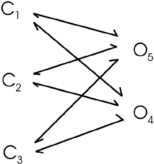
Besides the necessity to repeat fits with different initial parameters, it is important to check the optimality of the resultant model to avoid possible false solutions. An uncoupled but otherwise fully connected model, as illustrated in Scheme VI, can be used to obtain the theoretical best likelihood for an individual data set (Rothberg and Magleby, 1998; Gil et al., 2001; Kienker, 1989). A globally optimal fit should have its best likelihood comparable to this theoretical best likelihood for the same data set. The fit can be further validated by inspection of the resulting dwell-time distributions against the actual histograms. For two-dimensional distributions, the dependency plots have been shown to be a sensitive display for fractional difference between the number of observed interval pairs and the numbers expected from the model (Magleby and Song, 1992).

SCHEME VI.

The choice of dead times for missed events poses another problem. For data that is idealized with hidden Markov modeling, it is ∼2–3 times the sampling duration, irrespective of channel kinetics and noise. For data idealized with threshold crossing, the value varies with the extent of low-pass filtering. In practice, the dead time may have to be chosen retrospectively. With the dead time too large, the likelihood surface becomes flat, and the fitting tends to produce nonunique solutions, which is indicative of an upper limit to the dead time. With the current program, problems like these have to be addressed manually. It remains a challenge to automate the solutions.

Model-independent fitting

Although the approach has been described as a model-based fitting technique, it allows model-independent fitting as well. This could be useful in many cases, especially for studies of newly identified ion channels, where an explicit knowledge of the model is unavailable. Under such circumstances, the exponential-based one-dimensional and two-dimensional histogram fitting provides a good staring point. The acquired knowledge of the time constants of the components and their proportions is also essential to establishment of a full kinetic scheme.

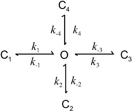
The equivalent exponential fittings can be achieved with the proposed approach using models of special topology. For one-dimensional histograms, a star model can be used. Fitting of a closed histogram with N components is equivalent to fitting the histogram using a model with N closed states connected to a single open state as in Scheme V.

SCHEME V.

The time constants of the components are the inverses of the opening rates, and the proportions are the relative frequencies of closures from the common open state; i.e.,

(35)

Since the proportion of a component is the area underneath it, the exponential coefficient of the component is given by

(36)

The fitting of an open histogram is essentially the same, with a star model consisting of a single closed state surrounded by as many open states as the expected number of exponential exponents.

The two-dimensional dwell-time distributions comprise two-dimensional exponentials with a total of 2N_cN_o degrees of freedom, where N_c and N_o are the number of closed and open components, respectively. The fitting of the two-dimensional histograms therefore requires a model involving the same number of parameters. One-such model is the fully connected but uncoupled one, as shown in Scheme VI.

The model is fully uncoupled, thereby ensuring its identifiability. The equivalent exponential fittings can be obtained by fitting the model to the two-dimensional dwell-time histograms, and then calculating the time constants and coefficients of the two-dimensional exponentials. The proportions of the individual two-dimensional components can be determined from the volume underneath each component.

The two-dimensional fitting described above assumes no knowledge of equilibrium. If the system is known at equilibrium, the rates of transitions that occur on a closed loop need to satisfy the detailed balance condition, which will lead to a reduction in the degrees of freedom of the model. This can potentially be used as a test for equilibrium. The fitting of two-dimensional histograms based on uncoupled models also alleviates the problem of handling constraints. With exponential fitting, there are a number of constraints that need to be imposed. These include the probability totality constraint and the constraints for self-consistency between marginal probabilities. Handling of these constraints is not straightforward as they are highly nonlinear in the parameters. With the use of a fully connected but uncoupled model, however, the constraints become implicitly satisfied.

Comparison to the full maximum-likelihood fitting

Although the one-dimensional histograms have limitations on the use of correlation information, the two-dimensional histograms, in theory, contain all information of the data for binary channels. This raises the question about the differences between the two-dimensional fitting and the full likelihood fitting of the dwell-time sequences, both of which utilize the correlation information between dwell-times.

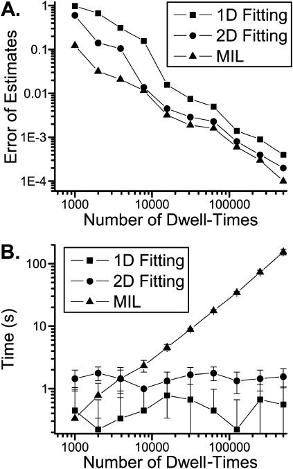
For comparison, data were simulated from the model in Scheme II, and the different fitting approaches were applied to re-estimate the rate constants. A dead time of t_d = 40 μs was used in all cases. Fig. 5 shows the mean deviations of the estimates from their true values and the corresponding time for each approach. The one-dimensional fitting is inadequate to resolve the model in general, but it nevertheless converged to the correct model given appropriate starting values. The full likelihood fitting has the least variances, which is in good agreement with the theory that the maximum likelihood approach is the most efficient estimator. For all three fittings, increasing data length reduces the estimation deviations, and the reduction is approximately inversed to the number of events. For this particular example, an ∼10% of mean error could be achieved with ∼4000 events for the two-dimensional histogram fitting and ∼8000 events for the one-dimensional fitting, respectively. Therefore, when the number of events is abundant, the histogram fitting could attain estimates with acceptable accuracy. On the other hand, the computational cost of both one-dimensional and two-dimensional fittings are independent of data length, whereas the time of the full likelihood fitting increases proportionally.

FIGURE 5.

Comparisons of the one-dimensional and two-dimensional histogram fittings with the full likelihood fitting of dwell-time sequences. (A) Mean errors of the estimates of parameters. Increasing data length reduced the estimation variances, and the reduction was approximately inversely proportional to the square-root of the number of events. The full likelihood fitting has the least variances among the three approaches, but the differences become relatively insignificant when the number of dwell-times is large. The mean errors are determined by where n is the number of rates, q-values are the true values of the rates used in simulation, and -values are the corresponding estimates. (B) Computational times of the fittings. The histogram fittings had a complexity virtually independent of data length, whereas the full likelihood approach increased proportionally. Analysis was based on data simulated from the five-state model for Ca²⁺-activated K⁺ channels in Scheme II. A dead time t_d = 40 μs was used throughout all tests. Results were averaged from 10 independent data sets, which were generated with different random seeds.

It should be noted that the histogram fitting applies only to channels at equilibrium. For channels that inactivate or with nonstationary stimuli, the full dwell-time sequence likelihood fitting has to be used. The analysis of these channels depends on the starting probability, and the time dependence of the data is lost after binning. In addition, histogram fitting, as described above, allows for data exhibiting only two conductance levels. The approach could be extended to multiple channels or single channels with substates, but there are usually a limited number of dwell-times for the high conductance levels, which may limit the quality of histograms, and in turn the accuracy of the estimates.

Model identification

The goal of kinetic analysis is the establishment of a model that can best describe the experimental data. Unfortunately, the problem has no analytical solution. It is relatively easy to find a model that gives the maximum likelihood at any single condition. For example, a fully connected and uncoupled model is always one of the candidates given a fixed number of states. The difficulty of the problem is to find a common model that gives the maximum likelihoods under all conditions.

One simple approach to the problem is perhaps an exhaustive search over all models. Although possible, the approach can be time-consuming even with the fast fitting procedure presented here. This is because the number of candidate models can be astronomically large even for a moderate size and it increases more than exponentially with the number of states. Therefore, it is always important to limit candidate models by making use of a priori information. The size of the model can be determined from the minimal number of components in the dwell-time distributions. Experience suggests that two-dimensional histograms provide more reliable estimates than one-dimensional histograms. Some components that are located close to each other in one-dimensional histograms may be separated in the two-dimensional histograms if their adjacent components are resolvable. The connections between the states are more difficult to determine and require comparisons of a large number of candidate models. Some aspects of the information may be deduced from the stimulus-dependence of the component results. For example, the components that remain at a saturated stimulus likely reside in the stimulus-independent regions of the model. The variability of the time constants of the components indicates whether the components are directly involved in stimulus-dependent transitions. Information may also come from other sources such as the structure of the channel and its biophysical and biochemical properties. In general, multiple sources of information have to be combined to reach a mechanistically coherent model.

References

- Ball, F. G., and M. S. P. Sansom. 1989. Ion-channel gating mechanisms: model identification and parameter estimation from single channel recordings. Proc. R. Soc. Lond. B Biol. Sci. 236:385–416. [DOI] [PubMed] [Google Scholar]
- Blatz, A. L., and K. L. Magleby. 1986. Correcting single channel data for missed events. Biophys. J. 49:967–980. [DOI] [PMC free article] [PubMed] [Google Scholar]
- Colquhoun, D., C. J. Hatton, and A. G. Hawkes. 2003. The quality of maximum likelihood estimates of ion channel rate constants. J. Physiol. 547:699–728. [DOI] [PMC free article] [PubMed] [Google Scholar]
- Colquhoun, D., and A. G. Hawkes. 1982. On the stochastic properties of bursts of single ion channel openings and of clusters of bursts. Philos. Trans. R. Soc. Lond. B Biol. Sci. 300:1–59. [DOI] [PubMed] [Google Scholar]
- Colquhoun, D., A. G. Hawkes, and K. Srodzinski. 1996. Joint distributions of apparent open and shut times of single-ion channels and maximum likelihood fitting of mechanisms. Philos. Trans. R. Soc. Lond. A Math. Phys. Eng. Sci. 354:2555–2590. [Google Scholar]
- Colquhoun, D., and F. J. Sigworth. 1995. Fitting and statistical analysis of single channel records. In Single-Channel Recording. B. Sakmann and E. Neher, editors. Plenum Publishing, New York. 483–587.
- Crouzy, S. C., and F. J. Sigworth. 1990. Yet another approach to the dwell-time omission problem of single-channel analysis. Biophys. J. 58:731–743. [DOI] [PMC free article] [PubMed] [Google Scholar]
- Fredkin, D. R., M. Montal, and J. A. Rice. 1985. Identification of aggregated Markovian models: application to the nicotinic acetylcholine receptor. Proc. Berkeley Conf. Neymann Kiefer.
- Gil, Z., K. L. Magleby, and S. D. Silberberg. 2001. Two-dimensional kinetic analysis suggests nonsequential gating of mechanosensitive channels in Xenopus oocytes. Biophys. J. 81:2082–2099. [DOI] [PMC free article] [PubMed] [Google Scholar]
- Hawkes, A. G., A. Jalali, and D. Colquhoun. 1990. The distributions of the apparent open times and shut times in a single channel record when brief events cannot be detected. Phil. Trans. R. Soc. Lond. A. 332:511–538. [DOI] [PubMed] [Google Scholar]
- Hawkes, A. G., A. Jalali, and D. Colquhoun. 1992. Asymptotic distributions of apparent open times and shut times in a single channel record allowing for the omission of brief events. Phil. Trans. R. Soc. Lond. B. 337:383–404. [DOI] [PubMed] [Google Scholar]
- Horn, R., and K. Lange. 1983. Estimating kinetic constants from single channel data. Biophys. J. 43:207–223. [DOI] [PMC free article] [PubMed] [Google Scholar]
- Hui, K. Y., B. Y. Liu, and F. Qin. 2003. Capsaicin activation of the pain receptor, VR1: multiple open states from both partial and full binding. Biophys. J. 84:2957–2968. [DOI] [PMC free article] [PubMed] [Google Scholar]
- Kienker, P. 1989. Equivalence of aggregated Markov models of ion-channel gating. Proc. R. Soc. Lond. B Biol. Sci. 236:269–309. [DOI] [PubMed] [Google Scholar]
- Magleby, K. L., and B. S. Pallotta. 1983. Calcium dependence of open and shut interval distributions from calcium-activated potassium channels in cultured rat muscle. J. Physiol. 344:585–604. [DOI] [PMC free article] [PubMed] [Google Scholar]
- Magleby, K. L., and L. Song. 1992. Dependency plots suggest the kinetic structure of ion channels. Proc. R. Soc. Lond. B Biol. Sci. 249:133–142. [DOI] [PubMed] [Google Scholar]
- Magleby, K. L., and D. S. Weiss. 1990a. Estimating kinetic parameters for single channels with simulation—a general method that resolves the missed event problem and accounts for noise. Biophys. J. 58:1411–1426. [DOI] [PMC free article] [PubMed] [Google Scholar]
- Magleby, K. L., and D. S. Weiss. 1990b. Identifying kinetic gating mechanisms for ion channels by using two-dimensional distributions of simulated dwell times. Proc. R. Soc. Lond. B Biol. Sci. 241:220–228. [DOI] [PubMed] [Google Scholar]
- Press, W. H., S. A. Teukolsky, W. T. Vetterling, and B. P. Flannery. 1992. Numerical Recipes in C. Cambridge University Press, Cambridge, UK.
- Qin, F., A. Auerbach, and F. Sachs. 1996. Estimating single channel kinetic parameters from idealized patch-clamp data containing missed events. Biophys. J. 70:264–280. [DOI] [PMC free article] [PubMed] [Google Scholar]
- Qin, F., A. Auerbach, and F. Sachs. 1997. Maximum likelihood estimation of aggregated Markov processes. Proc. R. Soc Lond. 264:375–383. [DOI] [PMC free article] [PubMed] [Google Scholar]
- Qin, F., A. Auerbach, and F. Sachs. 2000a. A direct optimization approach to hidden Markov modeling for single channel kinetics. Biophys. J. 79:1915–1927. [DOI] [PMC free article] [PubMed] [Google Scholar]
- Qin, F., A. Auerbach, and F. Sachs. 2000b. Hidden Markov modeling for single channel kinetics with filtering and correlated noise. Biophys. J. 79:1928–1944. [DOI] [PMC free article] [PubMed] [Google Scholar]
- Rothberg, B. S., and K. L. Magleby. 1998. Investigating single-channel gating mechanisms through analysis of two-dimensional dwell-time distributions. Meth. Enzymol. 293:437–456. [DOI] [PubMed] [Google Scholar]
- Roux, B., and R. Sauve. 1985. A general solution to the time interval omission problem applied to single channel analysis. Biophys. J. 48:149–158. [DOI] [PMC free article] [PubMed] [Google Scholar]
- Venkataramanan, L., and F. J. Sigworth. 2002. Applying hidden Markov models to the analysis of single ion channel activity. Biophys. J. 82:1930–1942. [DOI] [PMC free article] [PubMed] [Google Scholar]
- Wilkinson, J. H., and C. Reinsch. 1971. Linear algebra. In Handbook for Automatic Computation, Vol. II. Springer-Verlag, New York.
- Zheng, J., and F. J. Sigworth. 1997. Selectivity changes during activation of mutant Shaker potassium channels. J. Gen. Physiol. 110:101–117. [DOI] [PMC free article] [PubMed] [Google Scholar]