Studies of Proton Translocations in Biological Systems: Simulating Proton Transport in Carbonic Anhydrase by EVB-Based Models

Abstract

Proton transport (PTR) processes play a major role in bioenergetics and thus it is important to gain a molecular understanding of these processes. At present the detailed description of PTR in proteins is somewhat unclear and it is important to examine different models by using well-defined experimental systems. One of the best benchmarks is provided by carbonic anhydrase III (CA III), because this is one of the few systems where we have a clear molecular knowledge of the rate constant of the PTR process and its variation upon mutations. Furthermore, this system transfers a proton between several water molecules, thus making it highly relevant to a careful examination of the “proton wire” concept. Obtaining a correlation between the structure of this protein and the rate of the PTR process should help to discriminate between alternative models and to give useful clues about PTR processes in other systems. Obviously, obtaining such a correlation requires a correct representation of the “chemistry” of PTR between different donors and acceptors, as well as the ability to evaluate the free energy barriers of charge transfer in proteins, and to simulate long-time kinetic processes. The microscopic empirical valence bond (Warshel, A., and R. M. Weiss. 1980. J. Am. Chem. Soc. 102:6218–6226; and Åqvist, J., and A. Warshel. 1993. Chem. Rev. 93:2523–2544) provides a powerful way for representing the chemistry and evaluating the free energy barriers, but it cannot be used with the currently available computer times in direct simulation of PTR with significant activation barriers. Alternatively, one can reduce the empirical valence bond (EVB) to the modified Marcus' relationship and use semimacroscopic electrostatic calculations plus a master equation to determine the PTR kinetics (Sham, Y., I. Muegge, and A. Warshel. 1999. Proteins. 36:484–500). However, such an approximation does not provide a rigorous multisite kinetic treatment. Here we combine the useful ingredients of both approaches and develop a simplified EVB effective potential that treats explicitly the chain of donors and acceptors while considering implicitly the rest of the protein/solvent system. This approach can be used in Langevin dynamics simulations of long-time PTR processes. The validity of our new simplified approach is demonstrated first by comparing its Langevin dynamics results for a PTR along a chain of water molecules in water to the corresponding molecular dynamics simulations of the fully microscopic EVB model. This study examines dynamics of both models in cases of low activation barriers and the dependence of the rate on the energetics for cases with moderate barriers. The study of the dependence on the activation barrier is next extended to the range of higher barriers, demonstrating a clear correlation between the barrier height and the rate constant. The simplified EVB model is then examined in studies of the PTR in carbonic anhydrase III, where it reproduces the relevant experimental results without the use of any parameter that is specifically adjusted to fit the energetics or dynamics of the reaction in the protein. We also validate the conclusions obtained previously from the EVB-based modified Marcus' relationship. It is concluded that this approach and the EVB-based model provide a reliable, effective, and general tool for studies of PTR in proteins. Finally in view of the behavior of the simulated result, in both water and the CA III, we conclude that the rate of PTR in proteins is determined by the electrostatic energy of the transferred proton as long as this energy is higher than a few kcal/mol.

INTRODUCTION

Proton translocations (PTRs) play a major role in biochemistry in general and bioenergetics in particular (Ermler et al., 1994; Gennis, 1989; Mitchel, 1961; Okamura and Feher, 1992; Wikstrom, 1998). Molecular understanding of this issue is crucial for the elucidation of the action of ATPase (Girvin et al., 1998), bacteriorhodopsin (Luecke et al., 1999; Luecke, 2000; Royant et al., 2000; Sass et al., 2000), cytochrome c oxidase (Ostermeier et al., 1997; Yoshikawa et al., 1998), and other important systems.

The considerations of the molecular details of PTR processes have been quite challenging and controversial. Many workers followed the influential model of Nagle and co-workers (Nagle and Morowitz, 1978; Nagle and Mille, 1981) and assumed, at least implicitly, that PTR in biological systems can be described as a concerted transfer across a “proton wire” where the key control is provided by the orientation of the elements that constitute the wire (Berendsen, 2001; de Groot and Grubmuller, 2001; Kong and Ma, 2001; Law and Sansom, 2002; Murata et al., 2000; Nagle and Morowitz, 1978; Nagle and Mille, 1981; Sansom and Law, 2001; Tajkhorshid et al., 2002; Zeuthen, 2001). It is important to clarify in this respect that in Nagle's model the PTR is controlled by two steps, a HOP step where the proton is being transferred and a TURN step where the water file rearranges its orientation. It is thus assumed implicitly that the overall barrier for the PTR process involves the effect of these two steps. However, the electrostatic energy of the transferred proton was not considered and the emphasis was placed on the orientational effect (see also below). In view of the reliance on the orientational process in water, we will refer to this view as the “orientational control model”. This idea is consistent with the description of proton transfer (PT) in water and ice, where all the sites are equivalent. Recent interest (Schmitt and Voth, 1998; Vuilleumier and Borgis, 1999) in the identification of the exact mechanism of H⁺ diffusion in water (the so-called Grotthus mechanism; Agmon, 1995; Eigen, 1964; Zundel and Fritcsh, 1986) has probably strengthened the focus on the proton wire concept, although the issue of the reorientation of the environment has also been considered consistently.

A different perspective has been put forward by Warshel and co-workers (Sham et al., 1999; Warshel, 1979, 1986), where the key factor that controls PT in proteins in general and PTR in particular has been identified as the electrostatic free energy of the transferred charge (the water reorganization was also taken into account but this was done while considering the system with the proton present on the donor or acceptor state). According to this view, (which is based on microscopic empirical valence bond (EVB) simulations of PTR in proteins; Warshel, 1979, 1991) the reorganization of the proton donor and acceptor (in the absence of the proton) are of secondary importance relative to the change in solvation free energy along the proton transport path. Interestingly, theoretical studies of PTR in bacterial reaction centers (RC) and cytochrome c oxidase (Kannt et al., 1998; Lancaster et al., 1996; Okamura and Feher, 1992) have implicitly recognized the importance of electrostatic effects by focusing on the pK_a values of ionizable groups and/or internal water molecules (Sham et al., 1999). An interesting, related point was made recently by Williams (2002).

At this point it might be important to clarify that the electrostatic control idea referred to the electrostatic energy of the transferred proton and not to the electrostatic energy of the water molecules that has been indeed considered by the proponents of the orientational control model. In other words, the electrostatic control model emphasizes the change of the energy of the transferred proton upon moving between different sites of the channel. It seems to us that calculations that did not consider the charge of the transferred proton could not evaluate its electrostatic barrier and thus did not contain the main element of the electrostatic model. Another aspect of the electrostatic model has been the prediction that the barrier for PTR is controlled by the electrostatic energy of the transferred proton and that the barrier is proportional to this electrostatic energy. This view is incompatible with the orientational model that emphasized the orientation of the water file without the proton. In other words, almost all those who adopted the orientational model focused, at least implicitly in their discussions and pictures, on the orientation of the water file. This was based perhaps on the assumption that once the water file is oriented correctly the transfer of the proton is not rate limiting (see discussion in “Assessing the approximations used”). Apparently, the idea that the electrostatic energy of the transferred proton is a crucial element in the control of the PTR was considered to be problematic (Nagle and Mille, 1981). More specifically, it was assumed that the use of the electrostatic energies of the proton to estimate the free energy diagrams for PTR is incorrect, not realizing perhaps the fact that ΔG^‡ is close to ΔG⁰ (and linearly correlated) in cases of PT with a small separation between the donor and acceptor (Warshel, 1981; Åqvist and Warshel, 1993). Instead it was suggested that the “mobility measured in ice” should be used “to estimate the rate constants for fundamental conduction processes along hydrogen-bonded chains in proteins.” In this respect one may argue that the proton wire model formally includes energy states (Nagle et al., 1980) that resemble the states of the electrostatic model. However, the connection between these energies and the electrostatic free energy of the transferred proton were never made, nor evaluated. In fact, the states considered seem to correspond to orientational states rather than charge states (e.g., Fig. 2, a and b) in Nagle et al., 1980). Thus, we believe that there is a clear and fundamental difference between the orientational and electrostatic models.

FIGURE 2.

Comparing the autocorrelation of the energy gap for the full model for in water (black line) and the corresponding underdamped models. The simulations were done using γ = 30 ps⁻¹ and γ = 25 ps⁻¹ for S/A (gray line) and S/B (gray line with ▪), respectively.

The contrast between the two views of the control of PTR in biological systems has been illustrated in our recent study of the water/proton selectivity in aquaporin (Burykin and Warshel, 2003) where it was demonstrated that the selectivity is due to an electrostatic barrier and not to the orientation of the unprotonated water molecules. Interestingly, several research groups have now concluded that the electrostatic effect must play a major role (de Groot et al., 2003; Ilan et al., 2004; Jensen et al., 2003; Yarnell, 2004).

To examine whether the electrostatic control model is valid for general PTR processes, it is crucial to look for a system where the time dependence of the PTR is known experimentally (in aqauporin we only know that the PTR is blocked). Here one of the best benchmarks is provided by carbonic anhydrase III (CA III), because in this system we know the rate constant for PTR and its change with mutations (Silverman et al., 1993). Reproducing the observed trend by microscopic simulations can provide a very powerful way of distinguishing between different conceptual models. If, for example, we find that the PTR in CA III is controlled by the electrostatic energy of the transferred proton rather than the water orientation, we are one step forward. In view of this consideration we will focus here on CA III. We note, however, that this study addresses the general issue of PTR in proteins and simply considers CA III as a powerful benchmark. We believe that an approach that reproduces the rate in CA III from first principles will provide the correct tool for analyzing PTR in other systems. Conversely we believe that methods that cannot reproduce the PTR in CA III are not capable of modeling PTR in other proteins and channels (as long as these have a significant barrier). We also note that the PTR in CA III involves a chain of several water molecules and other donors and acceptors, thus making it relevant to other proton-conducting systems. Here it is significant that the free energy barrier for PTR in CA III is ∼10 kcal/mol, which is much lower than the ∼20 kcal/mol barrier in aquaporin (Burykin and Warshel, 2003) (which has been considered originally to reflect the water orientation effects) and quite close to the estimated ∼6 kcal/mol barrier in gramicidin A.

To obtain a molecular understanding of PTR in proteins and to resolve the above controversies, it is essential to be able to develop simulation methods capable of converting the available structural information about relevant systems to the corresponding observed kinetics. The method of choice for actual simulations is probably the EVB method. This method was developed in 1980 for studies of chemical reactions in proteins (Warshel and Weiss, 1980) and has been used extensively by our group and by others for simulations of PT in proteins and solution (for a recent review, see Warshel, 2003). It may be important to note that recent EVB versions (for a list of versions, see Florian, 2002) have basically the same ingredients as the original EVB model. This includes the MS-EVB model (Schmitt and Voth, 1998, 1999; Vuilleumier and Borgis, 1997, 1998) used in recent attempts to study PTR in proteins (Ilan et al., 2004). More specifically, the original EVB model (Warshel and Weiss, 1980) and many of its subsequent applications used multistate models and the main point, adopted in all EVB studies of reactions in proteins, is the introduction of the electrostatic potential of the environment in the EVB Hamiltonian. As clarified in the Methods section, this is not much different than, for example, an early MS-EVB study of PTR within six water molecules in water (Vuilleumier and Borgis, 1997). At any rate, the EVB provides a general combined quantum mechanical/molecular mechanics (QM/MM) method that can be applied for basically any process in condensed phases. Moreover, the EVB can be used and has been used extensively in quantitative studies of activation free energies for PT in proteins (e.g., Åqvist and Warshel, 1992, 1993; Warshel, 1991, 2003). The problem, however, is to evaluate the actual kinetics (and/or proton current) in cases with high activation barriers and many binding sites for the proton. In such cases it is practically impossible to use direct microscopic EVB simulations to reproduce the time-dependent PTR process, because this process can occur on a millisecond timescale. Thus it is important to develop related but simpler approaches.

Recently we developed semimacroscopic approaches that should allow one to simulate general PTR processes in proteins (Sham et al., 1999). This approach starts with the EVB formulation, which is then reduced to a simplified expression (a modified Marcus' formula) for the activation free energy for the PTR processes. The free energy changes needed for this treatment are then evaluated by semimacroscopic electrostatic calculations and the resulting calculated activation free energies and rate constants are used to evaluate the relevant kinetics by a master equation. However, this modified Marcus' approach involves several approximations that have not yet been verified by careful comparison to the corresponding microscopic results. Considering the effectiveness of the modified Marcus' approach, it seems to us that it is crucial to establish its general validity. It is also important to try to move from the master equation treatment to a more “molecular” time-dependent treatment that will also be closer to the full EVB treatment, but still allow us to study long-time PTR processes.

In view of the above considerations we developed in this work an approach that is halfway between the full EVB model and the modified Marcus' treatment. This model evaluates the effective free energy surfaces in terms of simplified EVB surfaces and then compares the results of Langevin dynamics (LD) on these surfaces with those obtained from explicit all-atom molecular dynamics (MD) simulations on actual EVB surfaces. The performance of our model is examined first by simulating PTR along a linear chain of EVB water molecules in water. It is shown that the rate of the PTR process depends exponentially on the free energy of the proton at the highest point of the free energy profile of a stepwise transfer process. With this finding in mind we move to the main challenge, which is the simulation of the PTR in CA III. It is found that the simplified EVB model reproduced the observed rate constant for PTR in CA III and in some mutants without adjusting any parameters for the protein calculation. This seems to establish the validity of our model and its applicability for general studies of PTR in proteins.

THE CA III SYSTEM

As stated in the introduction it is important to have a well-defined benchmark for studies of PTR processes in proteins. Unfortunately there are very few well-characterized systems where we know the starting initial and final position of the transferred proton and the corresponding transfer rate. Even in gramicidin A, it is not entirely clear what is the rate-limiting step of the PTR process (Decoursey, 2003). Fortunately, as will be shown below, CA III provides an excellent benchmark with clear structural information and well-studied rate constants for the PTR process (Silverman, 2000).

The catalytic reaction of CA III can be described in terms of two steps. The first is an attack of a zinc-bound hydroxide on CO₂ (Åqvist and Warshel, 1993; Silverman and Lindskog, 1988):

(1)

The reversal of this reaction is called the “dehydration step”. The second step involves the regeneration of the OH⁻ by a series of PT steps (Åqvist and Warshel, 1992; Silverman and Lindskog, 1988).

(2)

where (in the notation of Silverman et al., 1993), BH⁺ can be water, buffer in solution, or the protonated form of Lys-64 (other CAs have His in position 64). A groundbreaking study of Silverman and co-workers (Silverman et al., 1993) has determined the k_B for the native enzyme and its mutants. This provided an extremely clear benchmark for PTR in proteins. Obviously, a model that can reproduce the rate constant for PTR in this system is likely to provide a useful tool for general studies of PTR in biological systems. Conversely, models that cannot accomplish this task are not likely to describe correctly PTR in proteins. Here one of the obvious questions is whether the rate constant for PTR in proteins is determined by the free energy of the transferred proton or by the orientation of the unprotonated water molecules (note that the electrostatic free energy of the proton reflects the reorganization of the protein plus water system).

The subsequent sections will examine our ability to model the PTR in CA and will also address the general implications of our findings. It is important to note here that the CA III system is highly relevant to other systems that “conduct” protons because it includes several well-defined water molecules that have been considered as a proton wire (e.g., Cui and Karplus, 2003; Isaev and Scheiner, 2001; Silverman, 2000). In addition to the benefit of using CA III as a model for PTR in proteins, it is also useful to understand the nature of the proton shuttle in CA III to gain a better understanding of the action of this enzyme.

METHODS

Our initial goal is to provide a general potential surface for PT between all the relevant sites in a given biological system. Here we believe that currently the most effective way to describe PT in condensed phases is the EVB method (Warshel, 1991). Alternative ab initio QM/MM methods are still too slow to allow for reliable simulations of general PTR (see discussion in Warshel, 2003). The EVB method was used in many works and by many research groups, and its reliability has been demonstrated in studies of PT in proteins and solution (e.g., Åqvist and Warshel, 1992, 1993; Bala et al., 2000; Billeter et al., 2001; Feierberg and Åqvist, 2002; Hwang et al., 1988; Kim et al., 2000; Kong and Warshel 1995; Schmitt and Voth, 1998; Vuilleumier and Borgis, 1998a,b; Warshel and Weiss, 1980; Warshel, 1991, 2003). Thus we will not give here a description of the EVB method and refer the reader to the available literature and book (Warshel, 1991). We also would like to point out that the EVB program is implemented in the MOLARIS program (Chu et al., 2004). However, we will describe here the EVB for the case of n protonation sites (which are considered formally as bases) and one excess proton. In this case we describe the EVB quantum system in terms of diabatic states

(3)

where B_iH⁺ is the protonated form of the B_i protonation site (e.g., an H₃O⁺).

Now, the i-th diagonal element of the Hamiltonian of this system is described by a force-field-like function that describes the bonding within donors, the bond of the proton to the i-th base, as well as the nonbonded interactions in the system and its interactions with the surroundings (protein or water). More specifically, the diagonal elements are described by

(4)

where the b⁽ⁱ⁾ values and θ⁽ⁱ⁾ values are, respectively, the bond lengths and bond angles in the quantum mechanical system composed of the n bases and the excess protons. The r_k,k′ runs over all the nonbonded distances in the quantum system, and the q values are residual charges of the indicated atom in the given resonance state. The screening of the charge-charge interaction is introduced only for short distances (bonding distances) where the correct quantum mechanical description does not follow the classical prescription. The r⁻⁴ term represents an approximation for the inductive interaction between the solute charges. describes the interaction between the quantum system (the “solute”) in its i-th state and the surrounding classical system (the “solvent”) that includes water molecules and/or protein atoms. is the solvent-solvent classical potential surface. Finally, is the so-called “gas phase shift” that determines the relative energy of the diabatic states (Warshel, 1991). The off-diagonal elements (the H_ijs) are described by empirical functions that are fitted to experimental information and ab initio calculation, and the ground-state energy, E_g, is obtained by diagonalizing the EVB Hamiltonian.

(5)

More detail on the nature of the EVB matrix elements for different systems is given elsewhere (e.g., Åqvist and Warshel, 1993; Warshel, 1991). In this work we represent the cases where the bases are water molecules with a slightly modified version of the parameters used in reference (Štrajbl et al., 2002). In other cases (i.e., His, Lys, Asp, and Glu as proton acceptors) we adjusted previously used EVB parameters.

The EVB Hamiltonian represents the basis functions of Eq. 3, where the proton can be located on any of the sites of the “active space” (the part of the system that is described quantum mechanically). The rest of the system is described classically. At this point, it might be useful to clarify that the EVB and the so-called MS-EVB (Schmitt and Voth, 1998; Vuilleumier and Borgis, 1998a,b) that were so effective in studies of proton transport in water, are more or less identical. More specifically, the so-called MS-EVB includes typically six EVB states in the solute quantum mechanical (QM) region and the location of this QM region changes if the proton moves. The QM region is surrounded by classical water molecules (the molecular mechanics (MM)) whose effect is sometimes included inconsistently by solvating the charges of the gas phase QM region (this leads to inconsistent QM/MM coupling with the solute charges as explained in, e.g., Shurki and Warshel, 2003; Villa and Warshel, 2001). More recently the coupling was introduced consistently by adding the interaction with the MM water in the diagonal solute Hamiltonian. Now our EVB studies were performed repeatedly with multistate treatment (e.g., five states in Warshel and Russell, 1986) and this has always been done with a consistent coupling to the MM region. Thus the only difference that we can find between our EVB and the recent MS-EVB version is that our EVB studies did not update the location of the QM region during the simulations, because they dealt with processes in proteins, where the barrier is high, rather than with low barrier transport processes (so that the identity of the reacting region has not changed during the simulations. Also note that the MS-EVB simulations in proteins, which involve a limited number of quantum sites, do not change the QM region (e.g., Cuma et al., 2001) during the simulations. Finally, in cases of high barriers the change of the QM region is not useful, because the main issue is the ability to obtain a proper evaluation of the free energy associated with climbing the barrier. Thus we conclude that the EVB and MS-EVB are identical methods, although we appreciate the elegant treatment of changing the position of the QM region during simulations, which is a very useful advance in EVB treatments of processes with a low-activation barrier.

At this point, we would like to clarify that we view the full EVB treatment as a reliable, fully documented, and established method for simulating PTR in condensed phases. The MOLARIS program (Chu et al., 2004; Lee et al., 1993) can perform EVB calculations on any biological system. Thus the validity of the EVB is not the issue of this work. What we need here, however, is a simplified EVB-based model that will reproduce the results of the full EVB model (which treats the protein and solvent explicitly) in a much shorter simulation time, and allows for simulations of PTR processes in the microsecond range. The simplified model can be based on an effective potential that treats explicitly only the molecules that are involved directly in the PTR (the active space). In doing so, our first priority is to force the free energy functionals associated with each simplified EVB state (the microscopic Marcus' parabolas), at the given environment, to have the same minimum and similar curvature as the corresponding functionals of the full EVB model. In other words, using the full EVB treatment we describe the adiabatic ground-state free energy, Δg, for a PT between two sites by considering the free energy functionals (Δg₁ and Δg₂) associated with the diabatic energies (the ε₁ and ε₂) and mixing them by the off-diagonal element H₁₂. The results of such a treatment are described in Fig. 1 (the figure also defines the reorganization energy, λ₁₂, which will also be discussed below). Now when we construct the simplified EVB model we try to force its free energy functionals to overlap those obtained by the full model. This can be done quite effectively by representing the simplified EVB surface by the same type of solute surface as in Eq. 4, while omitting the solute-solvent and solvent-solvent terms (the U_Ss and U_ss terms) and modifying the Δ⁽ⁱ⁾ values to reflect the missing effect of the solvent. With this in mind we use here an effective Hamiltonian, of the form

(6)

The free energy, associated with the ground-state potential () of the simplified Hamiltonian, (here the free energy accounts for the average over the coordinates of the active space) is treated as the effective free energy surface that includes implicitly the rest of the system. In other words, we use

(7)

where r are the coordinates of the active space. Now the treatment of Eq. 6 provides a simple and powerful way of representing the energetics of the environment implicitly by adjusting the Δ⁽ⁱ⁾ values to the corresponding Δ̄⁽ⁱ⁾ values while imposing the requirement

(8a)

(8b)

where ( )_eff represents the quantity obtained with the effective EVB potential and ( )_complete designates the results obtained when the EVB treatment considers the entire system explicitly. For convenience we usually determine (and the corresponding Δ⁽ⁱ⁾ values of the effective model) by the semimacroscopic electrostatic calculations described below. At this point we would like to clarify that what is done to satisfy Eq. 8a is not some ad hoc treatment, but a well-defined procedure that exploits the fact that the EVB free energy functionals, g, change linearly with the gas phase shift (the Δ⁽ⁱ⁾). To satisfy Eq. 8b we need to have a similar curvature to the EVB functional of the simplified and the full model. Here we have two options. The first is to modify the solute potential (usually it is enough to change the D in the ε⁰ of Eq. 4) in the simplified model, and thus to change the solute reorganization energy to account for the effect of the reorganization energy of the missing solvent. The second option is to add effective solvent coordinates to the simplified model (both options will be used here).

FIGURE 1.

A description of the relationship between the diabatic free energy functions (g₁ and g₂), the adiabatic ground state free energy (g), the reorganization energy (λ), and the mixing term (H₁₂). The specific results are taken from EVB simulations of a PT step in CA III.

It is useful to note that in moving to the simplified models we try to keep the parameters in similar to those in the full model. However, because the solvent contribution is not included explicitly in we do not have the electrostatic screening effect of the solvent and we have to reduce the residual solute charges (see below). The effect of the solvent on the free energy functionals is, of course, still included by adjusting the Δ⁽ⁱ⁾ values and the parameters that determine the reorganizational energy.

Finally, to obtain a stable result we have to consider one more step. That is, the calculation of by the EVB/umbrella sampling (EVB/US) approach (Warshel, 1991) or by the related free energy perturbation approaches can be quite challenging due to convergence problems. Instead, we chose to use the semimacroscopic PDLD/S-LRA method (Lee et al., 1993; Schutz and Warshel, 2001) used effectively in our previous studies of PTR and ion transport (Burykin and Warshel, 2003; Sham et al., 1999). This approach describes the total free energy of each proton configuration as

(9)

where is the charge of the k-th group in the m-th configuration. The relevant pK_a values in the different sites of the protein are determined semimacroscopically by evaluating the change in solvation energy of moving the charged group from water to the given site (for a review of this approach, see Schutz and Warshel, 2001). Now the free energy of a proton transfer between site i and site j is given by Warshel (1981):

(10)

where is the change in the effective charge-charge interaction between the donor and acceptor upon PT and ε(R) is the effective dielectric constant for this interaction (at a charge separation R).

With the effective potential defined by Eqs. 6 and 7 above it is possible to examine the time dependence of PTR processes by Langevin dynamics (LD) simulations. That is, the time dependence of the system is determined by a Langevin equation (McQuarrie, 1976):

(11)

where is the effective potential of Eq. 7, i runs over the ions, α runs over the x, y, and z Cartesian coordinates of each ion, is the mass of the i-th ion, γ_i is the friction coefficient for the i-th ion, and A_iα is a random force, which is related to γ_i through the fluctuation-dissipation theorem (Kubo and Toyozawa, 1955).

The above LD treatment represents the effect of the solvent by modifying the solute reorganization energy and by the friction coefficient of Eq. 11. A more physically consistent treatment should include also an explicit effective solvent coordinate. The prescription for doing so is well known in the electron transfer community (e.g., Dakhnovskii and Ovchinnikov, 1986; Warshel and Parson, 2001), where the solvent coordinate, Q, is considered as the corresponding reaction field, or more microscopically by the electrostatic component of the energy gap (Hwang et al., 1988; Warshel, 1982). This type of solvent coordinate has been introduced to general studies of charge transfer reactions in the framework of a two-state EVB formulation (Hwang et al., 1988). For the benefit of the reader, we outline some elements of this treatment, but recommend reading (Hwang et al., 1988) for the details. Now in the two-state model, one can write

(12)

where the r and q are the actual “normal” coordinates of the solute and solvent molecules, whereas R and Q are the effective dimensionless coordinates for the solute and solvent, respectively. The effective frequencies ω_Q and ω_R are evaluated by in which P(ω) is the normalized power spectrum of the corresponding contribution to (ε₂ − ε₁). The R are related to the regular solute reaction coordinate R′ = (b₁ − b₂) by where μ_R is the reduced mass for the normal mode that is the compression of b₁ and extension of b₂. The reaction coordinate Q is defined in terms of the electrostatic contribution (ε₂ − ε₁)_el to (ε₂ − ε₁). Thus, we have Q = −(ε₂ − ε₁)_el/ℏω_Qδ_Q), which is also related to the dimensional solvent reaction coordinate, Q′, by Q = Q′(ω_Qm_Q/ℏ)^1/2. ΔV₀ is the difference between the minima of ε₂ and ε₁. Here we replace the contribution from each set of coordinates by one effective coordinate. The displacements (the δs) are related to the reorganization energy, λ, given by

(13)

An equivalent and more familiar definition of the solvent coordinate (see also Eq. 12) can be obtained in terms of the macroscopic reaction field (ξ_R) at the solute cavity, i.e., taking Q to be proportional to ξ_R we obtain

(14)

where μ₁ and μ₂ are the dipole moments of the solute for the corresponding diabatic states, and Q = ξ_‖/C (here ξ_‖ is the projection of ξ on (μ₁ − μ₂)). In the simple two state case we can obtain a convenient description of the dependence of the ground-state potential (Hwang et al., 1988) on the solvent coordinate using:

(15)

where μ is the adiabatic dipole moment of the solute. The derivatives of the ground-state potential with respect to R and Q gives a pair of coupled LD equations for the solute and solvent systems (see Hwang et al., 1988). Here we would like to adopt the above treatment, but we have to extend it to a multistate model that describes a chain of water molecules. This is done by writing

(16)

where is defined in Eq. 9 and where we assign two solvent coordinates to each state that corresponds to a proton inside the chain. In this way we have one coordinate (Q_i,k(i)) assigned to the i-th oxygen (which is protonated in state i) and to the subsequent oxygen, while assigning a second coordinate (Q_i,k′(i)) to the i-th oxygen and the oxygen before it. When i is the first oxygen, we do not have a Q_i,k′(i). In the case of only one pair of oxygens (only Q_i,k(i)), we have the same treatment as in Eqs. 12 and 15, except that we use δ instead of δ/2, for reasons that will be clarified below. Now when we consider the total energy of the system we can write

(17)

is the lowest eigenvalue of Eq. 5, and the B term expresses the coupling between the solvent coordinates. Here reflects the effect of the ε_is of Eq. 16, and the other terms in the equation reflect the cost in solvent-solvent energy associated with moving the solvent coordinates from their equilibrium position. This treatment is slightly different than the one used by (Hwang et al., 1988), because in that treatment the solvent-solvent repulsion was already incorporated in the δ values. As a result, this δ is given by Note that this relationship is different (by √2) than the standard relationship, due to the presence of the solvent term in Eq. 17.

Substituting Eq. 16 in Eq. 5 we obtain

(18)

where is the solute Hamiltonian (with as diagonal elements and the gas phase as off-diagonal elements) and C_g is the ground state eigenvector of the simplified EVB Hamiltonian (with the diagonal elements of Eq. 16). The corresponding LD equation for the solvent coordinate is now expressed as

(19)

where , whereas and m_Q are the effective friction and effective mass of the solvent. Here we replace the coupling between the solute dipole and the solvent reaction field (the term of Eq. 15) by the alternative expression, which is exact in the two-state case. Now, determines the amount of positive charge on the i-th site, and also plays the role of In the multistate case we introduce a significant approximation and consider independently the coupling of the solvent to each charge.

The parameter in Eq. 16 can be obtained from the power spectrum of the solvent fluctuations (see Hwang et al., 1988) and is obtained from the electrostatic contribution to the solvent reorganization energy, The friction coefficient, can be obtained (see Hwang et al., 1988) from the relationship where

(20)

In this work we considered two models; model S/A (where S designates simplified) only includes the solute coordinate (Eq. 11), whereas S/B considers the solute and solvent coordinate (Eqs. 11 and 19) simultaneously. Both models should reproduce the main dynamical and energetic features of the PTR process. Here we note that the dynamics of the PT processes are controlled by the fluctuation of the energy gap (Hwang et al., 1988; Warshel, 1984; Warshel and Parson, 2001). Thus we require that the autocorrelation of the energy gap for the active and complete systems will be similar. Thus, we required that

(21)

We also required that the effective dynamics of the proton transport process will be similar (similar residence time) in both the simplified and full models. For model S/A we obtained the best fit using and a.u. The performance in terms of satisfying Eq. 21 is described in Fig. 2, whereas other aspects are considered in “Simulating representative models”. The use of a large for H reflects the fact that this model tries to account simultaneously for the missing solvent fluctuations by the effective dynamics of the solute. In looking for the optimal parameters for model S/B we started by fixing the solute and considering only the solvent coordinate for both the simplified and full model. This gave with obtained from the power spectrum of the electrostatic energy gap of the full model for the solvated H₃O⁺ H₂O system (see discussion in Hwang et al., 1988), and obtained from the autocorrelation of the solvent contribution to the energy gap (Hwang et al., 1988). The fitting of both models also gave us a solvent reorganization energy, of 30 kcal/mol. The solvent effective mass was estimated by using the relationship that gave The values of and were then obtained by trying to satisfy Eq. 14 for both the total energy gap, where both the solute and solvent are free to move, and also by requiring that the time dependence of the proton transport (see below) will be similar in both models. A reasonable fit was obtained with and (see Fig. 2). Furthermore, we obtained an excellent fit between the λ_Q of the full model and model S/B.

In general, one could have tried to obtain different friction coefficients for different atoms. However, we obtained similar results while changing the γ values of the heavy atoms, and the next important improvement is the inclusion of the solvent coordinates. Another important issue is the friction used for the protein simulations. Here we used the same friction as in the water simulations, because the autocorrelation of the energy gap in the protein and in solution were found to be similar.

We would like to emphasize at this point that the exact value of the optimal dynamical parameters is not so crucial here because different parameters allow us to satisfy Eq. 21. More importantly, our main aim is to see if models that reproduce the approximated trend of the dynamics of the full model can be used to explore the dependence of the PTR rate on the free energy of the central proton. If we can establish a Boltzmann type dependence of the PTR rate on the electrostatic free energy of the transferred proton (with a reasonable range of parameters for the simplified model), and if we can capture such a trend with the full model (in the time range available for this model) we can gain some confidence in the validity of the electrostatic model. On the other hand, if we find “conduction band”-like PTR processes even with the large electrostatic barrier, then the orientational model is valid. It is also useful to note that it is harder to fit simultaneously the free energy surfaces and the dynamics of model S/A and the full model, than to do so with model S/B and the full model. Here the obvious difference is the fact that model S/B provides a much more realistic description of the solvent coordinate than model S/A. Nevertheless, having two different models allows us to be more certain about the validity of our conclusion.

The simulations that used the above parameters and the LD equations (Eqs. 11 and 19) were found to be too slow to allow us to obtain the relevant proton current in cases with high activation barriers. In such cases it might be advantageous to treat the system in the overdamped limit at the expense of having a large transmission factor. Thus we decided to use the overdamped LD approach (Schuss, 1980; van Gunsteren et al., 1981) of model S/A in studies of cases with high activation barriers. Now we obtained the optimal behavior (in terms of stability of the simulations) using For model S/B, we found the underdamped model to be sufficiently effective. In this case we took into account the incorrect “dynamical” effects by using the relationship

(22)

The scaling factor, S, reflects the change in transmission factor upon change from the underdamped to overdamped model (with the specific γ_H and ). The dependence of this factor on the activation barrier for the transfer process was evaluated using a model of six water (a, b, c, d, e, f) molecules where the pK_a of the two central molecules is being changed artificially to establish the desired activation barrier, Δg^‡. The ratio between the transmission factor of the two models was then determined, according to the prescription of Hwang et al. (1988), by running downhill trajectories (starting with a proton at the center of the system) and evaluating the average time of relaxing to H₂O_b or H₂O_e. This procedure gave S ≈ 16 for Δg^‡ ≈ 0, and S ≈ 7 for Δg^‡ > 4. This means that for the challenging high barrier case the overdamped and underdamped models gave similar rate constants, but the overdamped model requires less integration steps.

To examine actual PTR in proteins, we considered the K64H-F198D mutant of CA III as a model system (see Schutz and Warshel, 2004; Silverman et al., 1993; Silverman, 2000 for a discussion of this system). The starting configuration was taken from the x-ray structure of S-glutathiolated carbonic anhydrase III (Protein Data Bank identification code 1FLJ; Mallis et al., 2000) that was then “mutated” to the K64H-F198D mutant and relaxed in a long relaxation run (100 ps) while being subjected to distance constraints of 9 Å between the Zn⁺² ion and the N^ε nitrogen of His-64. This generated an “in” conformer for the histidine with a shorter chain of water molecules between the Zn⁺² ion and the histidine, and thus simplified the simulation and discussion. To construct the active space (the part included explicitly in the simplified models) we started by our regular procedure of embedding the protein in water and running a relaxation run (Lee et al., 1993). Next, we located all internal water molecules that can be involved in the PTR process and the protein groups that can participate in this process. Next we examined two options. In the first one, we kept all the internal water molecules and evaluated pK_a values of their protonated form by the PDLD/S-LRA approach. We then looked for the shortest network between the molecules with the highest pK_a (H₃O⁺). These molecules were then used as the active space of the simplified model with a Cartesian position restraint with K = 10 kcal·mol⁻¹·Å⁻². We also added a distance restraint of the form with K = 4 kcal·mol⁻¹·Å⁻² between the oxygens of nearby water molecules. In the second procedure we kept in the active space all internal water molecules that were a reasonable distance from each other, and then again, used the Cartesian restraint V′ upon moving to the simplified model. It was eventually concluded that the first model is sufficiently reliable for this set of calculations. The LD simulations were done with our MOLARIS simulation program (Chu et al., 2004; Lee et al., 1993), considering the given chain of donor and acceptors. The optimal time steps were 20 fs and 1 fs for the overdamped and underdamped models, respectively. All the PDLD/S-LRA calculations, including the MD simulation needed to generate the protein configurations for the LRA calculations, were performed using the MOLARIS package. Similarly, we used MOLARIS to perform the EVB calculations with the complete model. The EVB parameters for the full model were taken from our previous EVB studies of the autodissociation of water in water (Štrajbl et al., 2002) with minor modifications (see Table 1). The EVB parameters of the simplified models were similar to those of the full model, and the main changes (see Table 1) were: i), the reduction of D in the Morse potential of the O-H stretch (this was done to reduce the solute reorganization energy in model S/A so that the total reorganization energy would be similar to that of the full model, which includes the solvent. We also used, for convenience, the same D in model S/B, although here we could use higher D and different H₁₂. ii), The charges of the simplified model were reduced because this model does not include explicitly the screening effect of the surrounding environment.

TABLE 1.

EVB parameters used in different models

	Full model*					Model S/A					Model S/B
Bond parameters†	D		b0		β	D		b0		β	D		b0		β
OW-HW	120.0	0.988			2.0	50.0	0.988			2.0	50.0	0.988			2.0
OH-HH	80.0	0.988			2.2	50.0	0.988			2.0	50.0	0.988			2.0
EVB atom‡	Charges					Charges					Charges
OW	–	−0.80			–	–	−0.40			–	–	−0.40			–
OH	–	−0.65			–	–	−0.40			–	–	−0.40			–
HW	–	0.40			–	–	0.20			–	–	0.20			–
HH	–	0.55			–	–	0.20			–	–	0.20			–
Off-diagonal Hijs	A	α′	β′	γ′		A	α′	β′	γ′		A	α′	β′	γ′
H2O⋯H3O+	260.0	0.9	0.0	0.0	0.0	200.0	0.9	0.0	0.0	0.0	200.0	0.9	0.0	0.0	0.0

^*Only parameters that are different than those used in Strajbl et al., 2002 are listed.

^†O_W-H_W denotes a bond present in the neutral water molecules, O_H-H_H denotes the bonds in the hydronium ion.

^‡The W subscript indicates it is an atom type in water, the H subscript denotes it is an atom type in hydronium.

It should be noted that the above approach for calculations of the effective free energy can be augmented by considering an approximated expression for the ground-state free energy, and the activation free energy for PT steps, For example, with a simple two-state model (Fig. 1) we can obtain a very useful approximation to the curve. That is, using the above-mentioned free energy perturbation/umbrella sampling formulation we obtain the that corresponds to the E_g and the free energy functions (the ) that correspond to the surfaces. This leads to the approximated expression

(23)

where x is the generalized reaction coordinate, which is given by Now we can exploit the fact that the curves can be approximated by parabolas of equal curvatures (this linear response relationship was found to be valid by many microscopic simulations (e.g., Åqvist and Warshel, 1993) and write

(24)

where the reorganization energy, λ, (which is illustrated in Fig. 1) includes now both the solute and solvent contributions. Using Eqs. 23 and 24, one obtains our modified Marcus relationship (Åqvist and Warshel, 1993; Hwang et al., 1988; Warshel, 1991)

(25)

where is the free energy of the reaction, and H_ij is the off-diagonal term that mixes the two relevant states whose average value at the transition state are and respectively. The first term in this expression is the regular Marcus' equation (Marcus, 1964), which corresponds to the intersection of and at The second and third terms represent, respectively, the effect of H₁₂ at and

It is useful to point out that the same approach used to derive Eqs. 23 and 25 can be used to derive an expression for a concerted path in a three-state system. This can be easily done numerically by a 3 × 3 EVB equation with identical reorganization energies and with

(26)

where the coordinate system is defined in Fig. 3. This type of system will be discussed at the end of the next section.

FIGURE 3.

A two-dimensional representation of the free energy surface for a concerted PT. The figure considers the EVB results for the 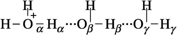system as a function of the O_α-H_α and O_β-H_β distances. The spacing of the contour lines is 3 kcal/mol. The figure demonstrates that the concerted path (α→γ) does not provide a lower barrier than the stepwise path (α→β→γ) in the typical case where and

SIMULATING REPRESENTATIVE MODELS

Before moving to calculations in proteins it is useful to establish the validity and performance of our approach in model systems. Thus we started this study by comparing the LD of the simplified model and MD of a complete model of a chain of six EVB water molecules embedded in a classical water sphere. The calculations were done for two cases, one with six identical water molecules (a, b, c, d, e, f) so that the PTR process involves a very small barrier and the second case where the gas phase shifts of the third and fourth water molecules are increased to simulate a decrease in the pK_a of H₃O⁺ in these positions. The simulated behavior of two such cases is considered in Figs. 4 and 5. Fig. 4 compares the calculated time dependence of the coefficients of the EVB wave function (the ) whose values tell us about the proton position. The time dependence for the of the full model (Fig. 4 a) corresponds to a picture where the proton spends 10 ps being delocalized on a specific pair of water molecules before moving to another (the average residence time over many trajectories was found to be ∼20 ps). This result is slower by about a factor of 10 from the ∼2 ps mean residence time anticipated from NMR experiments (see Vuilleumier and Borgis, 1998a,b). However, this is not a major concern for this work for the following reasons. i), A related overestimate was reported in an early EVB study and was attributed to the neglect of nuclear quantum mechanical (NQM) effects (Vuilleumier and Borgis, 1998b). Obviously, we could have followed the subsequent study of Borgis (Vuilleumier and Borgis, 1999) and improved the residence time of the model, but this would not have changed substantially any of the conclusions of this article. ii), This model considers a transfer along one direction in a three-dimensional water system. The rate of transfer in the case can be somewhat different than that obtained when the proton is allowed to move in all directions. iii), As noted above, the physics of our full EVB model is identical to that of the so-called MS-EVB model (Schmitt and Voth, 1998; Vuilleumier and Borgis, 1998a,b), and it is not essential to repeat their calculations. Thus, we only want to make sure that the parameterization of our full model gives reasonable results. More specifically, our point is not the validation of the full EVB model in bulk water, but the calibration of the simplified models that would reproduce the main properties of a reasonable full model. With this in mind, the main point of Fig. 4 is the similar behavior of the underdamped version of model S/A and the full model. We also show in Fig. 4 c that the transfer time of the overdamped version of model S/A is ∼16 times longer than that of the underdamped version. Similar behavior was obtained by model S/B.

FIGURE 4.

Comparing the time dependence of the probabilities of the different EVB states, (the ) of the (H₂O_a, H₂O_c, H₂O_d, H₂O_e, H₂O_f) model system (where ΔG_αβ = 0 kcal/mol for all PT steps) using the full model (a), the simplified model (S/A) in the underdamped (b) and overdamped limits (c). When a proton is localized on a given site, the corresponding is unity.

FIGURE 5.

Comparison of the time dependence of the probability amplitudes of the transferred proton for the (H₂O_a, H₂O_c, H₂O_d, H₂O_e, H₂O_f) model system, with ΔG_bc = ΔG_ed = 2 kcal/mol, using the full model (a), the simplified model (S/A) in the underdamped limit (b) and the overdamped limit (c). The coordinates are the same as those described in Fig. 4.

Next we start to consider our main point, which is the dependence of the average transfer rate on the electrostatic free energy of the transferred proton. Here we start with a case that can be simulated by the full EVB model (ΔG_ab = 0, ΔG_bc = ΔG_cd = 2, ΔG_de = 0). Now we find that the rate becomes slower, and that again the average transfer time of the overdamped model is ∼16 times longer than that of the underdamped model. A more general comparison was done by a systematic variation of the gas phase shifts of states c and d (or the corresponding pK_a values of the and ) evaluation of the resulting ΔG_b→d and by our EVB/US procedure and then calculations of the actual transfer time, τ_b→e for the full model and for models S/A and S/B. The results of this study are summarized in Fig. 6. As seen from the figure, once Δg^‡ is larger than 4 kcal/mol, the dependence of τ⁻¹ on Δg^‡ follows the trend predicted by transition state theory. That is, assuming that the frictional effects are independent of we can write

(27)

where we used the fact that

FIGURE 6.

Examining the relationship between the average time (in s) of transfer from b to e for different ΔG₀ values (ΔG_bc = ΔG_ed = ΔG₀). The figure describes the results of the full model and models S/A and S/B. The line with diamonds corresponds to the underdamped version of model S/A, squares to the overdamped version of model S/A, circles to the full model, and stars to the underdamped version of model S/B. The dashed line designates the trend predicted by transition state theory.

The above results were obtained for cases where the barrier for transfer between two water molecules involves two intervening water molecules. Another interesting case involves only one intervening water molecule. This case is less sensitive to the decrease of the pK_a of the central H₃O⁺ because of the fact that the concerted path helps to overcome the barrier of the stepwise path. This problem does not occur, however, with two intervening water molecules (see discussion in “Concluding remarks”).

Finally, we would also like to point out that we obtained the same trend in longer chains of explicit water molecules, including a chain of 12 molecules, which corresponds to the length of the water channel in gramicidin A.

SIMULATIONS OF PTR IN CA III

After verifying the performance of our approach in simple representative cases, we considered the PTR in CA III, which is our main benchmark. The groups that were considered in the active space are shown in Fig. 7. Of course, we could have considered explicitly more protein groups but this would not have changed our verification study (see below).

FIGURE 7.

The active space groups in the K64H-F198D mutant of CA III.

The first step of our simulation has been the evaluation of the free energies of protonation of the different protonation sites of the K64H-F198D mutant. The free energy for PT from the zinc-bound water to the next water molecule was evaluated previously (Åqvist and Warshel, 1992) by EVB calculations (because it requires a special treatment of the Zn⁺² ion). The free energies for all the subsequent steps were obtained by the PDLD/S-LRA approach. The corresponding results are given in dark lines in Fig. 8. We chose this mutant because it involves a relatively low barrier for PTR from site d to site a. Using these free energies we constructed the overall free energy profile for the simplified model using the standard EVB/US procedure (Warshel, 1991), but with the underdamped version of model S/A. In this procedure, we adjusted the gas phase shifts (the Δ⁽ⁱ⁾ values) to force the simulated ΔG_ij to reproduce the corresponding PDLD/S-LRA results (this corresponds to the use of Eqs. 8a and 10). The corresponding profile is also shown in Fig. 8. We also converted the PDLD/S-LRA results to the corresponding activation barriers for the PTR process using Eq. 25 with λ_ij = 80 kcal/mol, and H_ij = 20 kcal/mol, as was done recently (Schutz and Warshel, 2004). This led to results that were almost identical to those presented in Fig. 8. Similar results were also obtained by the EVB/US treatment of the complete model (not shown).

FIGURE 8.

Converting the PDLD/S-LRA results to an approximated EVB profile. The PDLD/S-LRA free energies of protonating each site (at pH = 7) are designated by bars, and the profiles for PT between different sites are designated by dashed lines. These profiles were evaluated by the EVB/umbrella sampling approach using the overdamped version of model (S/A). Similar results were obtained with the underdamped model.

Combining the above analysis and the conclusions from Fig. 6 indicates that the overall PTR is determined by the highest barrier and the corresponding ΔG_ij values. However, it is still crucial to establish that the frictional effects do not change the overall picture, and that our approach is capable of handling complex multisite kinetics. It is also crucial to establish that a proper multistate EVB treatment gives the same trend obtained by the modified Marcus' treatment. To establish these points, we used the simplified EVB and explored the PTR dynamics of the K64H-F198D mutant of CA III. In doing so, we explored first a PTR from His-64 to the zinc-bound OH⁻. The rate of this process should correspond to the k_B of Silverman et al. (1993). Because direct simulations took too long even with the overdamped model (about two weeks on an IBM Pentium III 1.13 GHz processor (Armonk, NY)) we pushed up the minimum at site d (His-64) by 1.2 kcal/mol, and obtained trajectories of the type presented in Fig. 9. This gave an average transfer time of

(28)

FIGURE 9.

The time dependence of the probability amplitude of the transferred proton for an LD trajectory for a PTR that starts at His-64 and ends at OH⁻ in the overdamped version of model S/A of the K64H-F198D mutant of CA III. The calculations were accelerated by considering a case where the minimum at site d is raised by 1.2 kcal/mol.

Correcting τ_d→a for the free energy shift (a factor of ∼7) and for the S factor of Eq. 22 (a factor of ∼7) gives now τ_d→a ≈ 7 × 10⁻⁷ s. This result is obtained assuming that the S factor in Eq. 22 is unity for large ΔG, and this assumption is probably not perfect. Thus, we consider the present result to be in a reasonable agreement with the time obtained from the experimentally observed k_B of our mutant (). To explore the effect of PTR from the bulk solvent, we also propagated trajectories from site f, which is close to the bulk solvent. Some trajectories bypassed the “trap” of His-64 and arrived at ∼10⁻⁹ s to site a (e.g., Fig. 10, which should be corrected to ∼10⁻⁸ s, considering the factor S of Eq. 22). Others were trapped by His-64, where it took ∼10⁻⁵ s to reach site a. Comparing the kinetic implications of these results to the corresponding observed pH profile is out of the scope of this work (it might also require averaging on different configurations of His-64). However, we note that the 10⁻⁹ s arrival time should be combined with the arrival time of a bulk proton, which is ∼2 × 10⁻⁵ s at pH = 7 (see Sham et al., 1999). At any rate, these results are very encouraging because they were obtained without adjusting any parameters in the protein calculations.

FIGURE 10.

The time dependence of the probability amplitude of the transferred proton for an LD trajectory for a PTR that starts at H₂O_f and ends at OH⁻ in the overdamped version of model S/A of the K64H-F198D mutant of CA III.

Although this simulation did not explore in a systematic way the observed effect of the different CA III mutants studied by Silverman (Silverman et al., 1993), it examined them in an indirect way. That is, our simulation of the rate of PTR from site d to site a shows a Boltzmann-type dependence on ΔG_d→a (the same type of dependence obtained in Fig. 6). Now we already have shown in a previous study that used the modified Marcus' treatment (Schutz and Warshel, 2004) that such a dependence reproduced the change of rate constants in the different mutants of CA III.

It may be useful to ask whether our simplified model captures the dynamical aspects of the full model of CA III. Obviously we cannot use a direct MD simulation and the full EVB model to explore the uphill PTR in CA, because this process involves activation barriers of >10 kcal/mol. However, we can still compare the performance of the full and simplified models in steps that involve small barriers. This was done by comparing the transfer from to His-64 in both models. As seen from Figs. 11 and 12, we obtained a similar transfer time in both cases.

FIGURE 11.

Showing the time dependence of the probability amplitudes of the transferred proton for a PTR trajectory of the complete model where the proton moves from to His-64 in the K64H-F198D mutant of CA III.

FIGURE 12.

Showing the time dependence of the probability amplitudes of the transferred proton for a PTR trajectory of the underdamped version of model S/A where the proton moves from to His-64 in the K64H-F198D mutant of CA III.

Before concluding this section, it might be useful to make a general comment about the energetics of concerted and nonconcerted PTR. The most important point in this respect is the finding that the stepwise and concerted mechanisms tend to follow a similar trend in endothermic processes (Štrajbl et al., 2002; Warshel and Weiss, 1980; Warshel et al., 1988). To see this point it is useful to consider Fig. 3 when and In this case we can exploit the fact that (when the proton donor and acceptor are at a close distance). With this we obtain

(29)

Thus the trend (and the dependence on ) is similar in both cases. Of course, when is much larger than the concerted path becomes more important, but this effect is taken into account in our considerations.

ASSESSING THE APPROXIMATIONS USED

In this work, as in any other simulation study, there are obviously some approximations. In assessing the validity and nature of these approximations we have to examine what we are trying to accomplish. That is, this work's starting point is that the full EVB model is a valid approach for reliable studies of PT in proteins. This view is based on the fact that the EVB is now used by many research groups (see Warshel and Florian, 2004 for a partial list) and is known to give accurate results in cases where the energetics of the PT process are known experimentally (e.g., Åqvist and Warshel, 1993). One may still wonder about the approximations in the full EVB method, but here the use of a semiempirical model in studies of proteins is as approximated as any of the current popular force-field methods, and does not need a special discussion. In fact the problem is frequently the convergence of the calculations and not the specific parameters (see Shurki and Warshel, 2003). With this in mind the next question is what are the approximations in the simplified model. Here it should be realized that the simplified model is only used as a tool for generating an EVB model that retains the physics of the full EVB model but does not include the solvent explicitly. Obviously this is an approximation, which is common to all implicit models, and it should be judged by the performance and by the physical constraints used. Now the approximations used for capturing the dynamics of the solvent, e.g., the friction and reduced mass are very reasonable, and at least in model S/B are very physical. Here the most important requirement is that the model will reproduce reasonable dynamics as judged by the autocorrelation of the energy gap (this autocorrelation has been shown to determine the dynamics of PTR processes (e.g., Warshel and Parson, 2001) and the average jump time, which is closely related to the diffusion time (Vuilleumier and Borgis, 1998b)). There are several sets of parameters that can give reasonable results and because the main issue is not the exact dynamics but the dependence on the energetics we feel that the parameters chosen are reasonable. Furthermore, by obtaining the same dependence on the energetics by two very different simplified models we believe that the approximations used to represent the effect of the environment of the solute dynamics are reasonable. Now let us move to the main issue, which is the dependence on the electrostatic energy of the transferred proton. Here we force the simplified EVB to be reliable by forcing the diagonal free energies to reproduce the free energy functionals of the full model (Eq. 8 and the discussion in Methods). Because it is very easy to satisfy Eq. 8, the reliability is judged by the reliability of the electrostatic free energy of the full system. Here we obtain a reasonable accuracy by using the PDLD/S-LRA model, whose reliability has been established by many studies, e.g., Schutz and Warshel (2001). In summary of this section, we do not feel that the approximations used here are particularly serious and it seems to us that this model is as reliable as the full model in terms of the dependence of the rate on the energetics, except that the simplified model allows us to examine processes that occur over a long time range. Furthermore, we can also double-check our approximation by comparing its results to those of the full model in processes that occur fast enough. Finally, as with any other approximated model, the only way to judge the reliability is to examine cases where the experimental result is known and to do this without adjustable parameters. On this count we are doing quite well.

CONCLUDING REMARKS

This work examined general aspects of PTR in proteins by considering such processes in CA III. To be able to perform simulations in a reasonable computer time in CA III, or in other systems with high activation barriers, we had to develop a simplified version of the EVB model. This was done by considering the given conduction chain as an “active space”, which is represented by an explicit EVB Hamiltonian, while accounting for the effect of the surroundings implicitly by changing the effective gas phase shift (the Δ̄⁽ⁱ⁾ of Eq. 6) and some of the solute force constants. The dynamical effects of the surrounding environment were modeled by using LD simulations. More specifically, the diagonal elements of the simplified model include a shift that forced the corresponding Marcus' parabolas to have the same minima as those of the full model. Similarly, the model was forced to reproduce the reorganization free energies and activation barriers of the full model by either adjusting the solute force constant (model S/A) or by adding effective solvent coordinates (model S/B). The dynamical properties of the simplified models were forced to approximate those of the full model by adjusting the effective friction so that the autocorrelation of the energy gap of the simplified models will be similar to that of the full model. The simplified models were then used in LD simulations of PTR processes, accounting in a physically consistent way for the delocalization of the proton charge and for possible concerted pathways. The validity of the simplified models was demonstrated first by comparing the corresponding simulations of PTR in a simple test case to those obtained in a fully microscopic EVB model. The simplified models, and in particular model S/A, were then used to simulate the PTR in CA III where it reproduced the observed rate constant without adjusting any parameters to obtain this result.

The establishment of the validity of our simplified model allows us to validate an even simpler EVB-based model, where the activation barriers for each PT step are evaluated by a modified Marcus formula. The relationship between this model and the simplified EVB model are demonstrated and clarified. This includes the issue of concerted pathways that will be further discussed below. It may also be useful to clarify that the recently developed Q-HOP model (de Groot et al., 2003; Lill and Helms, 2001) is related to our EVB-based model but without the well-defined physical origin. That is, the Q-HOP model followed the philosophy of our previous work (Sham et al., 1999) and tried to extend it to MD simulation of PTR in proteins. This was done by developing an empirical approximation to our Eq. 25 (see discussion in Lill and Helms, 2001 of their Eq. 3) but without the EVB basic formulation. In this way, it is hard to treat correctly delocalization effects and/or extend the model in a consistent way to concerted pathways. At any rate, both the simplified EVB and the modified Marcus' formulations can be applied to PTR in proteins, but the simplified EVB provides a more rigorous way to explore dynamical and frictional effects (that are nevertheless, less important than the energetics of the system).

The reliability of this study and other studies of PTR in proteins depend strongly on the reliability of the calculated energetics of the proton in the different protonation sites. Here we believe that the combination of the FEP/US calculations of the a→b step and the PDLD/S-LRA calculations of the other steps provide one of the most reliable options. As much as CA is concerned, we would like to point out that at present, only EVB studies (e.g., Åqvist and Warshel, 1992) provide a reasonable estimate of the observed k_cat. In this respect, it is instructive to clarify some possible misunderstandings due to the finding of recent gas phase ab initio calculations (e.g., Cui and Karplus, 2003; Isaev and Scheiner, 2001; Lu and Voth, 1998). For example, Cui and Karplus (2003) evaluated by ab initio density functional theory (DFT) calculations of the energy profile for PT between the Zn-bound water to His-64 in a gas phase model system with different numbers of bridging water molecules (two, three, and four bridging molecules). It was found that the gas phase energy profile changes drastically (from 0.6 to 6 kcal/mol) depending on the number of bridging water molecules (the point here is the change with the number of water molecules, and not the actual barrier). However, our PDLD/S-LRA and FEP simulation studies indicated that the above findings probably reflect an artifact of the use of gas phase calculations. Basically, the dielectric effect of the protein environment is a key factor. For example, the energy of the PT from a→b is critically dependent on the screening of the effect of the Zn⁺² ion on the OH⁻ (Åqvist and Warshel, 1992) and cannot be estimated correctly without taking into account the effect of the environment. The EVB gives a barrier of ∼10 kcal/mol for the a→b step and for the concerted a→c path (note that the value for a→b is taken from the accurate calculation of Åqvist and Warshel, 1992). This result is in a complete agreement with the corresponding experimental results. It is also useful to note that in contrast to frequent implications in the literature, (where it is implied that the isotope effect in CA is inconsistent with stepwise PTR) the observed isotope effect has been reproduced by the NQM centroid calculations of Hwang and Warshel (1996) (see also discussion in Schutz and Warshel, 2004). The full information content of the experimental isotope effect studies can only be extracted by performing NQM simulations for alternative pathways and different numbers of bridging water molecules. We are not aware of any such study, and it is not clear if such a study would provide unique conclusions. Finally, it might also be useful to comment on studies that reported gas phase ab initio calculations of the reaction of CA (Lu and Voth, 1998). These calculations assumed that the success of the quantitative 1992 EVB/FEP study of CA is fortuitous. However, EVB calculations are particularly effective in reproducing accurately the difference between reactions in solutions and proteins (or the effects of mutations in a given protein). Calibrating the EVB on the solution reaction does not leave much opportunity for fortuitous results.

One of the main reasons for the apparent difficulties of accepting the electrostatic control model has probably been associated with the concerted nature of PTR in solution. It has been assumed by some that the concerted motion can provide a way to overcome the electrostatic barrier that can exist for PTR in proteins. It is also possible that it has been assumed that the modified Marcus' formulation and perhaps our EVB model are restricted to a stepwise mechanism and to a two-state model. In this respect it is important to clarify that already our first EVB studies (e.g., Warshel and Weiss, 1980; Warshel et al., 1988) explored the concerted pathways and demonstrated that the energetics of the stepwise and the concerted paths are correlated in a similar way with the effect of the environment. This point has been established at the end of the section entitled “Simulations of PTR in CA III” with the help of Fig. 3, for the case when ΔG_α→β ≫ 0 and ΔG_β→γ ≈ 0. Thus it seems to us that different attempts to imply that the concerted path is fundamentally different than the stepwise path are inconclusive at best, unless they involve a comparison of the energetics of both paths (such a comparison has been done repeatedly by our group (e.g., Strajbl et al., 2000; Warshel and Weiss, 1980). The same is true with regards to attempts to use isotope effects to prove the importance of concerted paths (see above). At any rate, the EVB model can include as many states as needed and can be used in studies of concerted pathways (although it might require a more extensive mapping procedure). The simplified EVB model also allows us to take into account the full concerted space. Finally, we would like to clarify that we recognize the fact that PTR in proteins involve a partially concerted motion of properly oriented hydrogen bonds. However, the penalty of orienting the hydrogen bonds to the correct orientation is not large and, furthermore, since the same type of least energy path exists for different ΔGs, it is the magnitude of the ΔGs that controls the corresponding rate constants.

This work has established the importance of the electrostatic energy of the transferred proton (e.g., Fig. 6 and the simulations of CA III). The same conclusions were obtained for a PTR through long chains of water molecules in water, which can be viewed as models for PTR through proton wires in general channels. Similar but more intuitive arguments have been made in our previous works using the modified Marcus' model (e.g., Sham et al., 1999). Nevertheless, the appreciation of the overwhelming contribution of electrostatic effects to PTR has been slow perhaps because of the picture that emerged from the influential model of Nagle and co-workers (Nagle and Morowitz, 1978; Nagle and Mille, 1981). This model, that was adopted implicitly in computational studies of PTR in gramicidin channels (e.g., Pomes and Roux, 1998, 2002), in membranes (e.g., Marrink et al., 1996), and in some respects, in the early discussion of aquaporin, divides the PTR process into two steps, a HOP step where the proton is being transferred and a TURN step where the water file rearranges its orientation. It was thus assumed implicitly that the overall barrier for the PTR process involves the effect of these two processes. Furthermore, since studies of PTR in membranes (e.g., Marrink et al., 1996) and other systems (Pomes and Roux, 1998, 2002) concluded that the TURN step is rate limiting in the specific systems studied, it was thus implied that the reorientation of the water file plays a major role in the overall PTR. This picture sometimes overlooked the solvation effect (e.g., moving from water to a less polar environment) on the HOP step and led, perhaps unintentionally, to the assumption that the reorganizational fluctuations of a single-file water chain in the absence of the proton in PT models can be used to estimate the overall barrier for a PTR process (again, the barrier is defined here as the overall activation barrier). Thus, it was implied that the free energy of inverting the directionality of the water file is directly relevant to the activation free energy of the overall PTR process. For example, an interesting work (Pomes and Roux, 1998) that addressed the “free energy for H⁺ conductance along hydrogen-bonded chains of water molecules” has concluded that “the inversion of the total dipole moment (of the unprotonated water file) involves an activation energy of ∼8 kcal/mol, whereas in contrast “the rapid translocation of an excess H⁺ across a chain extending between two spherical solvent droplets is an activationless process.” This finding was probably brought forth as a study that is relevant to gramicidin and other channels, and obviously the conclusion implies that the free energy barrier is mainly influenced by the water reorientation. The origin of this misunderstanding might be due to calculations of PTR without sufficient water molecules on both sides of the channel, thus obtaining a barrierless PTR step. Related attempts to consider the actual gramicidin channel (Pomes and Roux, 2002) were also put forward as a support of the Nagle proton wire mechanism. However, the calculations were restricted again to the center of the channel, thus overlooking the key problem (which is the energy for moving from bulk water to the channel).

Regardless of the issue of the contribution of the H⁺ translocation step, it is also important to recognize that the separation into HOP and TURN steps is problematic. That is, while separating the two steps may be reasonable in studies of PTR in water, it does not provide a proper computational or conceptual prescription when one deals with cases with significant electrostatic barriers. In such cases the relevant free energy should have been considered by evaluating the free energy of the proton on each site and the solvent reorganization energy (considering the presence of an actual proton). As was shown in many of our early studies of this problem (e.g., Åqvist and Warshel, 1993) and in this work, the correct adiabatic barrier associated with the (large) solvent reorganization energy is quite small for small separation between the donor and acceptor (due to the effect of H₁₂) and thus the key factor is In other words, calculations of the free energy profile for overall dipolar reorientation in the absence of the proton (e.g., Pomes and Roux, 1998) are not related directly to the energetics of the PT process and we are not aware of any formulation that established such a relationship in a consistent way. On the other hand, the EVB provides a relatively rigorous framework that relates the protein (or solvent) dipolar reorganization to the free energy profile for the PT process. This formulation (e.g., Eqs. 23 and 25) tells us exactly what type of reorganization energy, should be considered in any specific PT step. The assumption that the complete reorganization of the water file in the absence of the proton is related directly to the energetics of the PTR process is somewhat problematic even in the framework of a thermodynamic cycle that would augment the calculations of the reorientation of the file by evaluating the energy of bringing the proton to the oriented file. First, the reaction coordinate for orienting the file does not correspond to the proper orientation of the file in each step of the PTR. In fact, the PT process only requires a perfect orientation of a few water molecules. Thus, for example, the configurations that promote a PT between two water molecules in the center of the channel do not require a special orientation of the entire water file. Instead they are correlated with the maximal solvation of the reactant and product states (the maximal solvation does not require a “head to tail” orientation of all the molecules along the water file). Realizing this point is particularly important when one proposes that the protein prevents a perfect orientation of the file, and that this prevents PTR (e.g., de Groot and Grubmuller, 2001). Second, any attempt to calculate separately the electrostatic energy of orienting the water molecules without the proton and then a separate evaluation of the electrostatic energy of the proton in the particular site would involve a “double counting” unless one evaluates correctly the electrostatic energy of binding the proton to the oriented water file (rather than to the relaxed solvent structure). As clarified in this work, with a consistent EVB formulation, a proper calculation should evaluate the electrostatic free energy of bringing the proton to a given site. Once this would be done, the free energy of the PT process will be determined by the reorganization free energy of both the channel polar groups and the water file, as well as by H_ij. Introducing alternative inconsistent approaches may lead to an incorrect picture.

In view of the fact that PTR processes in water sometimes involve transfer between clusters it is natural to wonder how we can deal with such processes while considering zero-order H₃O⁺states. The answer is that the time dependence of the EVB eigenvectors (the Cs of Eq. 5) describes any form of PTR. If the process involves a transfer of it will be reflected in the corresponding Cs. The problem in realizing this point might reflect confusion between the basis set used (the isolated, localized H₃O⁺ of Eq. 3) and the actual states obtained from their mixing. Thus it is important to realize that the EVB considers the entire system (while incorporating, of course, all the field from the protein in the diagonal Hamiltonian) and then mixes the diagonal states. This means that the delocalization is obtained after the addition of the environment rather than before. This appears to be a somewhat more rigorous and physically consistent treatment than molecular orbital QM/MM. It is also important to realize that the issue of transfer of delocalized clusters becomes much less important once we have high barriers for the PTR process. That is, the EVB Hamiltonian (which provides an excellent description of the system) stops giving a delocalized picture once the energy of the isolated states go uphill. Now, on the flat region of the barrier we again may have delocalized states but their energy would be determined by the energy of the localized states. For example, the EVB produces delocalized states on the top of the barrier of aquaporin but this is irrelevant to the overall barrier because there is no delocalized state that moves the proton without a barrier from one side of the channel to another. The belief that this should be the physics of PTR in channels and proteins is perhaps the reason why the electrostatic model was rejected for a long time. At any rate, it is useful to view the PTR issue by thinking of an EVB matrix where the diagonal energies reflect the electrostatic barrier and its fluctuations. With such a model one finds that once the energies of state i + 1 and i + 2 are significantly higher than that of state i, it will be found that the PTR is controlled by ΔG_i+1. Only when the energies of all states are similar will we find that the transfer is controlled by the Grotthuss mechanism.

The use of the simplified EVB model is particularly effective in cases with high barriers and many protonation sites. However, after identifying the key pathways we can still refine the transmission factor along different high-energy plateaus by more rigorous approaches. For example, it is possible to use the full EVB model and to run downhill trajectories from different high-energy points. Comparing the corresponding paths and transmission factors can tell us if we have to modify the conclusions from the simplified model.

Our simulations of the PTR in CAIII were accelerated by raising the minimum at site d by ∼1.2 kcal/mol to reduce the computational time. Such a controlled change of the reaction landscape can be used as a general strategy in more complex PTR problems. Alternatively, it might be useful to accelerate the calculations by increasing the simulation temperature.

Some workers considered the time of forming different water configurations as a key factor in the rate of PTR (e.g., Marrink et al., 1996). Although this is unlikely to be a crucial factor in our system, it might be important in some cases where the solvent is not present in the transfer path before the transfer process (this is equivalent to the well-known issue of the Marcus' work function). Moreover, a more systematic study of CA III should have considered several alternative configurations of the donor at residue 64. Thus it might be useful to evaluate the free energy of forming different water configurations and/or different configurations of the residues that participate in the PT process. Once this is done we can obtain the overall rate constant by running the simplified EVB simulations from these configurations and averaging the results according to the probability of the initial configurations. Note, however, that we are not talking here on minor configurational changes around a given conformational state, because the PDLD/S-LRA procedure can handle this effect and provides the free energy of the proton in each conformational state.

As established in this and previous works (e.g., Schutz and Warshel, 2004) the key parameter that controls PTR is the electrostatic energy of the proton on the different bases along the transfer pathway. Evaluating these energies or the corresponding pK_a values is the key prerequisite for reliable simulations of PTR in proteins. Thus, one can and should judge different strategies for simulations of PTR in proteins by their ability to reproduce reliable pK_a values. In this respect, we view the simplified EVB method as a particularly promising approach, considering the demonstrated reliability and consistency of the PDLD/S-LRA treatment. Of course, one can also use the complete EVB FEP/US approach to evaluate the proton transfer free energies, but it is not clear that this can give more reliable pK_a values. At any rate, we believe that this simplified approach offers a general and extremely effective way for studying PTR in proteins.

References

- Agmon, N. 1995. The Grotthuss mechanism. Chem. Phys. Lett. 244:456–462. [Google Scholar]
- Åqvist, J., and A. Warshel. 1992. Computer simulation of the initial proton transfer step in human carbonic anhydrase I. J. Mol. Biol. 224:7–14. [DOI] [PubMed] [Google Scholar]
- Åqvist, J., and A. Warshel. 1993. Simulation of enzyme reactions using valence bond force fields and other hybrid quantum/classical approaches. Chem. Rev. 93:2523–2544. [Google Scholar]
- Bala, P., P. Grochowski, K. Nowinski, B. Lesyng, and J. A. McCammon. 2000. Quantum-dynamical picture of a multistep enzymatic process: reaction catalyzed by phospholipase A2. Biochem. J. 79:1253–1262. [DOI] [PMC free article] [PubMed] [Google Scholar]
- Berendsen, H. J. C. 2001. Reality simulation: observe while it happens. Science. 294:2304–2305. [DOI] [PubMed] [Google Scholar]
- Billeter, S. R., S. P. Webb, P. K. Agarwal, T. Iordanov, and S. Hammes-Schiffer. 2001. Hydride transfer in liver alcohol dehydrogenase: quantum dynamics, kinetic isotope effects, and role of enzyme motion. J. Am. Chem. Soc. 123:11262–11272. [DOI] [PubMed] [Google Scholar]
- Burykin, A., and A. Warshel. 2003. What really prevents proton transport through aquaporin? Charge self-energy versus proton wire proposals. Biophys. J. 85:3696–3706. [DOI] [PMC free article] [PubMed] [Google Scholar]
- Chu, Z. T., J. Villa, M. Strajbl, C. N. Schutz, A. Shurki, and A. Warshel. 2004. MOLARIS version beta 9.05. Los Angeles, CA.
- Cui, Q., and M. Karplus. 2003. Is a “proton wire” concerted or stepwise? A model study of proton transfer in carbonic anhydrase. J. Phys. Chem. B. 107:1071–1078. [Google Scholar]
- Cuma, M., U. W. Schmitt, and G. A. Voth. 2001. A multi-state empirical valence bond model for weak acid dissociation in aqueous solution. Journal of Physical Chemistry A. 105:2814–2823. [Google Scholar]
- Dakhnovskii, Y. I., and A. A. Ovchinnikov. 1986. Adiabatic electron transfer in polar media quantum transition state theory. Mol. Phys. 58:237–252. [Google Scholar]
- Decoursey, T. E. 2003. Voltage-gated proton channels and other proton transfer pathways. Physiol. Rev. 83:475–579. [DOI] [PubMed] [Google Scholar]
- de Groot, B. L., T. Frigato, V. Helms, and H. Grubmuller. 2003. The mechanism of proton exclusion in the aquaporin-1 water channel. J. Mol. Biol. 333:279–293. [DOI] [PubMed] [Google Scholar]
- de Groot, B., and H. Grubmuller. 2001. Water permeation across biological membranes: mechanism and dynamics of aquaporin-1 and GlpF. Science. 294:2353–2357. [DOI] [PubMed] [Google Scholar]
- Eigen, M. 1964. Proton transfer, acid-base catalysis, and enzymatic hydrolysis. Part I: Elementary processes. Angew. Chem. Int. Ed. Engl. 3:1–19. [Google Scholar]
- Ermler, U., G. Fritzsch, S. K. Buchanan, and H. Michel. 1994. Structure of the photosynthetic reaction centre from Rhodobacter sphaeroides at 2.65 Å resolution: cofactors and protein-cofactor interactions. Structure. 2:925–936. [DOI] [PubMed] [Google Scholar]
- Feierberg, I., and J. Åqvist. 2002. The catalytic power of ketosteroid isomerase investigated by computer simulation. Biochemistry. 41:15728–15735. [DOI] [PubMed] [Google Scholar]
- Florian, J. 2002. Comment on molecular mechanics for chemical reactions. J. Phys. Chem. A. 106:5046–5047. [Google Scholar]
- Gennis, R. B. 1989. Biomembranes: molecular structure and function. Springer-Verlag, New-York, NY.
- Girvin, M. E., V. K. Rastogi, F. Abildgaard, J. L. Markley, and R. H. Fillingame. 1998. Solution structure of the transmembrane H+-transporting subunit c of the F1F0 ATP synthase. Biochemistry. 37:8817–8824. [DOI] [PubMed] [Google Scholar]
- Hwang, J.-K., G. King, S. Creighton, and A. Warshel. 1988. Simulation of free energy relationships and dynamics of SN2 reactions in aqueous solution. J. Am. Chem. Soc. 110:5297–5311. [Google Scholar]
- Hwang, J.-K., and A. Warshel. 1996. How important are quantum mechanical nuclear motions in enzyme catalysis? J. Am. Chem. Soc. 118:11745–11751. [Google Scholar]
- Ilan, B., E. Tajkhorshid, K. Schulten, and G. A. Voth. 2004. The mechanism of proton exclusion in aquaporin channels. Proteins. In press. [DOI] [PubMed]
- Isaev, A., and S. Scheiner. 2001. Proton conduction by a chain of water molecules in carbonic anhydrase. J. Phys. Chem. B. 105:6420–6426. [Google Scholar]
- Jensen, M. O., E. Tajkhorshid, and K. Schulten. 2003. Electrostatic tuning of permeation and selectivity in aquaporin water channels. Biophys. J. 85:2884–2899. [DOI] [PMC free article] [PubMed] [Google Scholar]
- Kannt, A., R. D. Lancaster, and H. Michel. 1998. The coupling of electron transfer and proton translocation: electrostatic calculations on Paracoccus dentrificans cytochrome c oxidase. Biophys. J. 74:708–721. [DOI] [PMC free article] [PubMed] [Google Scholar]
- Kim, Y., J. C. Corchado, J. Villà, J. Xing, and D. G. Truhlar. 2000. Multiconfiguration molecular mechanics algorithm for potential energy surfaces of chemical reactions. J. Chem. Phys. 112:2718–2735. [Google Scholar]
- Kong, Y., and G. Ma. 2001. Dynamic mechanisms of the membrane water channel aquaporin-1 (AQP1). Proc. Natl. Acad. Sci. USA. 98:14345–14349. [DOI] [PMC free article] [PubMed] [Google Scholar]
- Kong, Y., and A. Warshel. 1995. Linear free energy relationships with quantum mechanical corrections: classical and quantum mechanical rate constants for hydride transfer between NAD+ analogues in solutions. J. Am. Chem. Soc. 117:6234–6242. [Google Scholar]
- Kubo, R., and Y. Toyozawa. 1955. Application of the method of generating function to radiative and non-radiative transitions of a trapped electron in a crystal. Prog. Theor. Phys. 13:160–182. [Google Scholar]
- Lancaster, C. R. D., H. Michel, and B. Honig. 1996. Calculated coupling of electron and proton transfer in the photosynthetic reaction center of Rhodopsedomonas viridis. Biophys. J. 70:2469–2492. [DOI] [PMC free article] [PubMed] [Google Scholar]
- Law, R. J., and M. S. P. Sansom. 2002. Water transporters: how so fast yet so selective? Curr. Biol. 12:R250–R252. [DOI] [PubMed] [Google Scholar]
- Lee, F. S., Z. T. Chu, and A. Warshel. 1993. Microscopic and semimicroscopic calculations of electrostatic energies in proteins by the POLARIS and ENZYMIX programs. J. Comp. Chem. 14:161–185. [Google Scholar]
- Lill, M. A., and V. Helms. 2001. Compact parameter set for fast estimation of proton transfer rates. J. Chem. Phys. 114:1125–1132. [Google Scholar]
- Lu, D., and G. A. Voth. 1998. Proton transfer in the enzyme carbonic anhydrase: an ab initio study. J. Am. Chem. Soc. 120:4006–4014. [Google Scholar]
- Luecke, H. 2000. Atomic resolution structures of bacteriorhodopsin photocycle intermediates: the role of discrete water molecules in the function of this light-driven ion pump. Biochim. Biophys. Acta. 1460:133–156. [DOI] [PubMed] [Google Scholar]
- Luecke, H., B. Schobert, H. T. Richter, J. P. Cartailler, and J. K. Lanyi. 1999. Structure of bacteriorhodopsin at 1.55 angstrom resolution. J. Mol. Biol. 291:899–911. [DOI] [PubMed] [Google Scholar]
- Mallis, R. J., B. W. Poland, T. K. Chatterjee, A. R. Fisher, S. Darmawan, R. B. Honzatko, and T. A. Thomas. 2000. Crystal structure of S-glutathiolated carbonic anhydrase III. FEBS Lett. 482:237–241. [DOI] [PubMed] [Google Scholar]
- Marcus, R. A. 1964. Chemical and electrochemical electron transfer theory. Annu. Rev. Phys. Chem. 15:155–196. [Google Scholar]
- Marrink, S. J., F. Jahnig, and H. J. Berendsen. 1996. Proton transport across transient single-file water pores in a lipid membrane studied by molecular dynamics simulations. Biophys. J. 71:632–647. [DOI] [PMC free article] [PubMed] [Google Scholar]
- McQuarrie, D. A. 1976. Statistical Mechanics. Harper and Row, New York, NY.
- Mitchel, P. 1961. Coupling of phosphorylation to electron and hydrogen transfer by a chemi-osmotic type of mechanism. Nature. 191:144–148. [DOI] [PubMed] [Google Scholar]
- Murata, K., K. Mitsuoka, T. Hiral, T. Waltz, P. Agrel, J. B. Heymann, A. Engel, and Y. Fujiyoshi. 2000. Structural determinants of water permeation through aquaporin-1. Nature. 407:599–605. [DOI] [PubMed] [Google Scholar]
- Nagle, J. F., and M. Mille. 1981. Molecular models of proton pumps. J. Chem. Phys. 74:1367–1372. [Google Scholar]
- Nagle, J. F., M. Mille, and H. J. Morowitz. 1980. Theory of hydrogen bonded chains in bioenergetics. J. Chem. Phys. 72:3959–3971. [Google Scholar]
- Nagle, J. F., and H. J. Morowitz. 1978. Theory of hydrogen bonded chains in bioenergetics. Proc. Natl. Acad. Sci. USA. 75:298–302. [DOI] [PMC free article] [PubMed] [Google Scholar]
- Okamura, M. Y., and G. Feher. 1992. Proton transfer in reaction centers from photosynthetic bacteria. Annu. Rev. Biochem. 61:861–896. [DOI] [PubMed] [Google Scholar]
- Ostermeier, C., A. Harrenga, U. Ermler, and H. Michel. 1997. Structure at 2.7 A resolution of the Paracoccus denitrificans two-subunit cytochrome c oxidase complexed with an antibody FV fragment. Proc. Natl. Acad. Sci. USA. 94:10547–10553. [DOI] [PMC free article] [PubMed] [Google Scholar]
- Pomes, R., and B. Roux. 1998. Free energy profiles for H+ conduction along hydrogen-bonded chains of water molecules. Biophys. J. 75:33–40. [DOI] [PMC free article] [PubMed] [Google Scholar]
- Pomes, R., and B. Roux. 2002. Molecular mechanism of H+ conduction in the single-file chain of the gramicidin channel. Biophys. J. 82:2304–2316. [DOI] [PMC free article] [PubMed] [Google Scholar]
- Royant, A., K. Edman, T. Ursby, E. Pebay-Peyroula, E. M. Landau, and R. Neutze. 2000. Helix deformation is coupled to vectorial proton transport in the photocycle of bacteriorhodopsin. Nature. 406:645–648. [DOI] [PubMed] [Google Scholar]
- Sansom, M. S. P., and R. J. Law. 2001. Aquaporins: channels without ions. Curr. Biol. 11:R71–R73. [DOI] [PubMed] [Google Scholar]
- Sass, H. J., G. Buldt, R. Gessenich, D. Hehn, D. Neff, R. Schlesinger, J. Berendzen, and P. Ormos. 2000. Structural alterations for proton translocation in the M state of wild-type bacteriorhodopsin. Nature. 406:649–653. [DOI] [PubMed] [Google Scholar]
- Schmitt, U. W., and G. A. Voth. 1998. Multistate empirical valence bond model for proton transport in water. J. Phys. Chem. B. 102:5547–5551. [Google Scholar]
- Schmitt, U. W., and G. A. Voth. 1999. The computer simulation of proton transport in water. J. Chem. Phys. 111:9361–9381. [Google Scholar]
- Schuss, Z. 1980. Theory and applications of stochastic differential equations. In Wiley Series in Probability and Mathematical Statistics. John Wiley & Sons, New York, NY. 321.
- Schutz, C. N., and A. Warshel. 2001. What are the dielectric “constants” of proteins and how to validate electrostatic models. Proteins Struct. Funct. Genet. 44:400–417. [DOI] [PubMed] [Google Scholar]
- Schutz, C. N., and A. Warshel. 2004. Analyzing free energy relationships for proton translocations in enzymes: carbonic anhydrase revisted. J. Phys. Chem. B. 108:2066–2075. [Google Scholar]
- Sham, Y., I. Muegge, and A. Warshel. 1999. Simulating proton translocations in proteins: probing proton transfer pathways in the Rhodobacter sphaeroides reaction center. Proteins. 36:484–500. [PubMed] [Google Scholar]
- Shurki, A., and A. Warshel. 2003. Structure/function correlations of proteins using MM, QM/MM and related approaches: methods, concepts, pitfalls and current progress. Adv. Protein Chem. 66:249–312. [DOI] [PubMed] [Google Scholar]
- Silverman, D. N. 2000. Marcus rate theory applied to enzymatic proton transfer. Biochem. Biophys. Acta. 1458:88–103. [DOI] [PubMed] [Google Scholar]
- Silverman, D. N., and S. Lindskog. 1988. Catalytic mechanism of carbonic anhydrase. Acc. Chem. Res. 21:30–36. [Google Scholar]
- Silverman, D. N., C. Tu, X. Chen, S. M. Tanhauser, A. J. Kresge, and P. J. Laipis. 1993. Rate-equilibria relationships in intramolecular proton transfer in human carbonic anhydrase III. Biochemistry. 34:10757–10762. [DOI] [PubMed] [Google Scholar]
- Strajbl, M., G. Hong, and A. Warshel. 2002. Ab-initio QM/MM simulation with proper sampling: “first principle” calculations of the free energy of the auto-dissociation of water in aqueous solution. J. Phys. Chem. B. 106:13333–13343. [Google Scholar]
- Strajbl, M., Y. Y. Sham, J. Villà, Z. T. Chu, and A. Warshel. 2000. Calculations of activation entropies of chemical reactions in solution. J. Phys. Chem. B. 104:4578–4584. [Google Scholar]
- Tajkhorshid, E., P. Nollert, M. Jensen, L. Miercke, R. M. Stroud, and K. Schulten. 2002. Control of the selectivity of the aquaporin water channel by global orientational tuning. Science. 296:525–530. [DOI] [PubMed] [Google Scholar]
- van Gunsteren, W. F., H. J. C. Berendsen, and J. A. C. Rullmann. 1981. Stochastic dynamics for molecules with constraints. Brownian dynamics of n-alkanes. Molecular Physics. 44:69–95. [Google Scholar]
- Villa, J., and A. Warshel. 2001. Energetics and dynamics of enzymatic reactions. J. Phys. Chem. B. 105:7887–7907. [Google Scholar]
- Vuilleumier, R., and D. Borgis. 1997. Molecular dynamics of an excess proton in water using a non-additive valence bond force field. J. Mol. Struct. 436–437:555–565. [Google Scholar]
- Vuilleumier, R., and D. Borgis. 1998a. An extended empirical valence bond model for describing proton transfer in H+(H20)n clusters and liquid water. Chem. Phys. Lett. 284:71–77. [Google Scholar]
- Vuilleumier, R., and D. Borgis. 1998b. Quantum dynamics of an excess proton in water using an extended empirical valence-bond Hamiltonian. J. Phys. Chem. B. 102:4261–4264. [Google Scholar]
- Vuilleumier, R., and D. Borgis. 1999. Transport and spectroscopy of the hydrated proton: a molecular dynamics study. J. Chem. Phys. 111:4251–4266. [Google Scholar]
- Warshel, A. 1979. Conversion of light energy to electrostatic energy in the proton pump of Halobacterium halobium. Photochem. Photobiol. 30:285–290. [DOI] [PubMed] [Google Scholar]
- Warshel, A. 1981. Calculations of enzymic reactions: calculations of pKa, proton transfer reactions, and general acid catalysis reactions in enzymes. Biochemistry. 20:3167–3177. [DOI] [PubMed] [Google Scholar]
- Warshel, A. 1982. Dynamics of reactions in polar solvents. semiclassical trajectory studies of electron-transfer and proton-transfer reactions. J. Phys. Chem. 86:2218–2224. [Google Scholar]
- Warshel, A. 1984. Dynamics of enzymatic reactions. Proc. Natl. Acad. Sci. USA. 81:444–448. [DOI] [PMC free article] [PubMed] [Google Scholar]
- Warshel, A. 1986. Correlation between structure and efficiency of light-induced proton pumps. In Methods in Enzymology. L. Packer, editor. Academic Press, London. 578–587.
- Warshel, A. 1991. Computer Modeling of Chemical Reactions in Enzymes and Solutions. John Wiley & Sons, New York, NY.
- Warshel, A. 2003. Computer simulations of enzyme catalysis: methods, progress, and insights. Annu. Rev. Biophys. Biomol. Struct. 32:425–443. [DOI] [PubMed] [Google Scholar]
- Warshel, A. and J. Florian. 2004. The empirical valence bond (EVB) method. In The Encyclopedia of Computational Chemistry. P.R. Schreiner, editor. John Wiley & Sons, Chichester, UK.
- Warshel, A., and W. W. Parson. 2001. Dynamics of biochemical and biophysical reactions: insight from computer simulations. Q. Rev. Biophys. 34:563–679. [DOI] [PubMed] [Google Scholar]
- Warshel, A., and S. Russell. 1986. Theoretical correlation of structure and energetics in the catalytic reaction of trypsin. J. Am. Chem. Soc. 108:6569–6579. [Google Scholar]
- Warshel, A., F. Sussman, and J.-K. Hwang. 1988. Evaluation of catalytic free energies in genetically modified proteins. J. Mol. Biol. 201:139–159. [DOI] [PubMed] [Google Scholar]
- Warshel, A., and R. M. Weiss. 1980. An empirical valence bond approach for comparing reactions in solutions and in enzymes. J. Am. Chem. Soc. 102:6218–6226. [Google Scholar]
- Wikstrom, M. 1998. Proton translocation by bacteriorhodopsin and heme-copper oxidases. Curr. Op. Struct. Biol. 8:480–488. [DOI] [PubMed] [Google Scholar]
- Williams, R. P. J. 2002. The problem of proton transfer in membranes. J. Theor. Biol. 219:389–396. [DOI] [PubMed] [Google Scholar]
- Yarnell, A. 2004. Blockade in the cell's waterway. Chem. Eng. News. 82:42–44. [Google Scholar]
- Yoshikawa, S., K. Shinzawa-Itoh, R. Nakashima, R. Yaono, E. Yamashita, N. Inoue, M. Yao, M. J. Fei, C. P. Libeu, T. Mizushima, H. Yamaguchi, T. Tomizaki, and T. Tsukihara. 1998. Redox-coupled crystal structural changes in bovine heart cytochrome c oxidase. Science. 280:1723–1729. [DOI] [PubMed] [Google Scholar]
- Zeuthen, T. 2001. How water molecules pass through aquaporins. Trends Biochem. Sci. 26:77–78. [DOI] [PubMed] [Google Scholar]
- Zundel, G., and J. Fritcsh. 1986. The Chemical Physics of Solvation, Vol. 2, Chap 2. Elsevier, Amsterdam, The Netherlands.