Kinetics of Filament Bundling with Attractive Interactions

Abstract

We study the kinetics of filament bundling by variable time-step Brownian-dynamics simulations employing a simplified attractive potential based on earlier atomic-level calculations for actin filaments. Our results show that collisions often cluster in time, due to memory in the random walk. The clustering increases the bundling opportunities. Small-angle collisions and collisions with short center-to-center distance are more likely to lead to bundling. Increasing the monomer-monomer attraction decreases the bundling time to a diffusional limit, which is determined by the capture cross-section and diffusion coefficients. The simulations clearly show that the bundling process consists of two sequential phases: rotation, by which two filaments align parallel to each other; and sliding, by which they maximize their contact length. Whether two filaments bundle or not is determined by the competition between rotation to a parallel state and escape. Increasing the rotational diffusion coefficient and attraction enhances rotation; decreasing attraction and increasing the translational diffusion coefficients enhance escape. Because of several competing effects, the filament length only affects the bundling time weakly.

INTRODUCTION

Polyelectrolytes such as DNA and F-actin often aggregate or bundle together in vivo or in vitro (Kawamura and Maruyama, 1970; Baeza et al., 1987; Bloomfield, 1996, 1997; Tang and Janmey, 1996; Tang et al., 1996). The aggregation of very long DNA molecules allows them to be stored in a very small volume. The bundling of actin filaments can enhance their rigidity, which is crucial for their cytoskeletal role of supporting cell extensions, and may affect the internal mechanical properties of the cell as well. On the other hand, the formation of amyloid fibrils, which are stable, ordered, filamentous protein aggregates consisting of multiple bundled protofilaments (Rochet and Lansbury, 2000), cause amyloidoses including many neurodegenerative diseases. Although there have been many theoretical studies in this field (Oosawa, 1968; Ray and Manning, 1994; Grønbech-Jensen et al., 1997; Ha and Liu, 1997; Kornyshev and Leikin, 1998; Shklovskii, 1999; Gelbart et al., 2000; Stevens, 2001; Diehl et al., 2001; Moreira and Netz, 2001; Deserno and Holm, 2002; Lau and Pincus, 2002; Manning, 2003), most of these have focused on deriving the attractive interaction between like-charged polymers. When the attractive interaction is mediated by counterions or bundling proteins, it is generally found to be short-ranged. Much less attention has been paid to the bundling process itself. Despite some theoretical studies of the thermodynamics of bundling (van der Schoot and Odijk, 1992; Sear, 1997; Khokhlov and Semenov, 1985; Yu and Carlsson, 2003), there has been no comprehensive theoretical analysis of bundling kinetics. There have been several experimental studies of bundling as a function of properties such as counterion concentration and filament length (Tang and Janmey, 1996; Tang et al., 1996), but we are not aware of systematic experimental studies of the bundling kinetics of filaments with short-ranged attractive interactions. Our purpose in this article is to establish the mechanism of bundling and develop simplified mathematical models of the bundling kinetics.

The realistic study of biopolymer bundling is often hampered by the absence of suitable interaction potentials. In our previous work (Yu and Carlsson, 2003), we derived the potentials between actin filaments in counterion solutions and simplified the attractive potential under a limited counterion concentration range as a sum of short-ranged monomer-monomer interactions. With this simplified potential, we studied the thermodynamics of bundling. The potentials of this form include the main features of the filament interaction: large anisotropy, short range, and steric exclusion. In this article, we use potentials of this form to reveal the bundling mechanism and to study its kinetics by Brownian dynamics simulations. The simulations are carried out under periodic boundary conditions, using variable time steps. Simplified mathematical models are then used to explain and summarize the simulation results.

METHODS

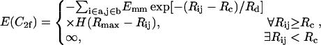
Our simplified attraction potential between two actin filaments in a two-filament conformation C_2f is of the form (Yu and Carlsson, 2003)

(1)

where a and b are two filaments containing monomers i and j, respectively; R_ij is the distance between the centers of i and j; R_d is a decay length (R_d = 7 Å); R_max is the distance cutoff for this short-ranged interaction; and H(x) is the Heaviside step function, which equals 0 for x < 0 and 1 for x ≥ 1. The monomers are arranged in a straight line. Eq. 1 implies that the bundling energy for parallel filaments varies fairly linearly with filament length. We let the monomer-monomer interaction vanish for R_ij > R_max (100 Å), and the closest approach distance allowed is R_c = 75 Å, the filament diameter. Any step leading to steric overlap (i.e., R_ij < R_c) is rejected in our Brownian dynamics simulations. E_mm is the maximal attractive energy of two monomers when they are in closest contact. The E_mm value found for attraction mediated by divalent metal ions at 32 mM is 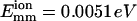(Yu and Carlsson, 2003), which may increase when mediated by bundling proteins such as fascin. Other aspects of the interaction may also be changed by bundling proteins. Note that the lowest energy for two filaments of equal length L (measured in monomers) is ∼−2LE_mm instead of −LE_mm, because a monomer can interact with more than one monomer in the other filament. Eq. 1 neglects the long-ranged interactions. Even for a simple system consisting of only two similarly charged plates and their counterions (no salt), the long-ranged monopolar repulsion is generally neutralized by the fluctuation-driven attraction (Lau and Pincus, 2002). In not-too-dilute salt solutions, the interaction will be short-ranged due to Debye-Hückel screening. As shown below, the short-ranged interaction simplifies the simulations greatly, because we can use large time steps when two filaments are far away from each other.

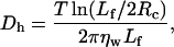
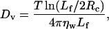
We use Brownian dynamics to simulate the filament motion, with diffusion coefficients calculated according to Doi and Edwards (1986). The three diffusion coefficients are

(2)

(3)

and

(4)

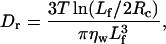
where D_h and D_v characterize the diffusion parallel and perpendicular to the filament, and D_r is the rotational coefficient. L_f is the filament length (L_f = L × 27.3 Å, where 27.3 Å is the height of a monomer), η_w is the dynamic viscosity of water, T is the temperature, and our temperature units are such that Boltzmann's constant is unity.

We carry out simulations in a periodic-boundary cubic cell (Fig. 1). One filament is chosen as the target, and this filament moves through other filaments, called environmental filaments. These constitute a solution of the desired filament concentration. Thus, we divide the whole space into periodic-boundary cubic cells, whose size is determined by the filament concentration, and fix an environmental filament at the center of each cell. The orientations of the environmental filaments could be assigned randomly for each filament, but we fix them in the z direction. This does not affect the results noticeably if the solution is dilute, and simplifies the treatment of steric exclusion. The target filament is initially put at a random position with a random orientation.

FIGURE 1.

The Brownian dynamics simulations are carried out under periodic boundary conditions, with variable time steps. One filament is chosen as the target (marked T), which moves through other environmental filaments (marked E), centered in cells. Environmental filaments are frozen; target filament moves relative to the environmental filament at the center of its cell.

Because the environmental filaments are frozen, the motion of the target filament should be taken as its motion relative to the environmental filament at the center of the same cell, i.e., its own motion with that of the central filament subtracted. Its own motion includes two parts: translation and rotation. To explain how we calculate the filament motion, we consider a horizontal filament for simplicity. 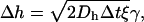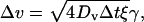Then translation has two directions: horizontal ĥ (along the filament) and vertical (perpendicular to the filament), where ĥ and are unit vectors. For each time step Δt, is randomly chosen from the directions perpendicular to the filament. The random displacements along ĥ and can be expressed as

(5)

(6)

where γ = ±1 defines the direction of the random Brownian motion, and ξ is a random variable, which satisfies We choose ξ randomly from 0 to 2. The values of γ and ξ are different in Eqs. 5 and 6, and change in every step. Thus, the translation step is

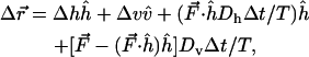(7)

where F is the force, driving the motion described by the last two terms.

To treat rotation, we define θ as the angle between the filament axis and the z axis, and φ as the corresponding azimuthal angle. The rotation is also divided into two components,

(8)

(9)

where 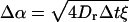is the magnitude of a random angle change and ψ is the angle between and ê_φ (the direction of φ), which is randomly chosen from 0 to 2π so that the direction of is random. τ_θ and τ_φ are torques driving rotation in the ê_θ (direction of θ) and ê_φ directions. When θ = 0, Δφ is randomly chosen from 0 to 2π. Similarly, we obtain the motion of the central environmental filament. By subtracting the motion of the central filament from the target filament's motion, we obtain the relative motion. Defining Δθ_c, and Δφ_c to be the translation and rotation of the central filament, we subtract its motion by two steps. First, we rotate the target filament by −Δθ_c about from the center of the central filament, where and are the directions of the x and y axes. Then we move the target filament by We ignore rotation about the filament axis because in our model the filament is isotropic. As mentioned above, any step leading to steric overlap is rejected.

The variable time step is chosen to depend as follows on the minimal monomer-monomer distance between two filaments, For d_ff > 120 Å, where 120 Å is an outer cutoff distance, Δt = max(Δt₀, (d_ff−120)²/(D_h × 10⁵)). This form guarantees that the target filament can move 100 steps without reaching d_ff = 100 Å, the contact distance. The time Δt₀ is the basic step used for d_ff < 120 Å. It is chosen so that the deterministic part of the motion is much less than the random part of the motion, in the presence of the interfilament force, and the energy change during a time step is much less than kT. This results in Δt₀ decreasing with increasing E_mm, and in our simulations, the Δt₀ values range from 3 to 30 ps. When the filaments contact and align parallel to each other, even very small motions can cause steric overlap so that almost all motion steps are refused. To solve this problem, we separate the motion of the target filament into three independent parts when they contact and align parallel to each other. The three parts are: rotation, sliding along and translation in the x, y plane. Although most of the rotations cause steric overlap, most sliding steps and a substantial part of the translation steps in the x, y plane will be accepted. We also decrease the time step by a factor of 15 when the interaction energy reaches 40% of its lowest value.

The bundling criteria are that the interaction energy of two filaments reaches 90% of its lowest value and the z difference is <5 Å. Generally, the sliding time is very short (∼10⁻⁵ s), and changing the 90% criterion to 80% affects the bundling time only slightly if the filament is not too short.

RESULTS

We run 150 bundling trajectories (or more) to obtain the average bundling times. Most of the simulations are carried out in the 4-μm × 4-μm × 4-μm cell, and the corresponding filament concentration is 2.596 × 10⁻¹¹ M. We also vary the filament concentration to evaluate its effect on the average bundling time. Our calculations show that the bundling rate (defined as the inverse of the average bundling time) is proportional to the filament concentration, as expected.

Time distribution of collisions

Collisions are prerequisite for bundling. We define a collision as beginning when d_ff < 100 Å (contact distance) and ending when d_ff > 120 Å (escape distance). Decreasing the escape distance increases the number of collisions (n_c). When the escape distance equals 100 Å, n_c increases abruptly and depends strongly on the time step. For larger escape distances, n_c does not depend on the time step. We chose 120 Å because it is consistent with our scheme for adjusting the time step. Changing this value does not affect our results significantly.

Fig. 2 shows the number of collisions N_c before time t for typical bundling runs using two different interaction strengths. We see that filaments with weak attraction require more time, and also many more collisions, to bundle: 303 for and 9 for 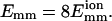The collisions tend to form clusters, as previously observed by Northup and Erickson (1992). They called the collision clusters encounters, and we will also use this terminology.

FIGURE 2.

Number of collisions n_c before time t for two simulation trajectories. (Solid line) ; (dotted line) L = 25 for both lines. Their lowest interaction energies are −0.269 eV (−10.4 kT) and −2.15 eV (−83.1 kT), respectively.

The clustering of collisions is caused by the random-walk memory, as we discuss in the Appendix. A particle in a random walk tends to return to its original position with a probability density proportional to exp [−r²/(4Dt)], which can be considered as coming from a pseudo-potential −Tr²/(4Dt), where r is the distance to the original position, D is its diffusion coefficient, and t is the time. The resulting clustering increases the contact time so that the filaments have more opportunities to rotate and find the right orientation for bundling. This increases the expected bundling rate by an approximate factor of s_e (the number of collisions in an encounter) if the orientations between neighboring collisions are not strongly correlated. For example, assuming that only a fraction 0.01 of collisions lead to bundling due to the orientation requirement, it is expected that the bundling rate for s_e = 1 will be 0.01 of the rate obtained without the orientation constraint; but if s_e = 100, the bundling rate will be almost the same as that without the orientation constraint. In Fig. 2, when although the bundling probability per collision is 1/9, the rate is the same as if the bundling probability were 1 because the first and ninth collisions occur almost at the same time. Previous studies (Schlosshauer and Baker, 2002) found that for sticking angular constraints of ∼5−15° of two balls, the reaction rate is ∼2−3 orders-of-magnitude higher than expected from a simple geometric model. Earlier calculations also showed that the reduction in reaction rate caused by orientation requirements is significantly less than suggested by the reduction in the probability for a properly oriented collision (Šolc and Stockmayer, 1971, 1973; Schmitz and Schurr, 1972; Shoup et al., 1981; Zhou, 1993).

We define an encounter as a cluster of collisions with the time spacing between all sequential collisions as <0.1 s. Within the same encounter, neighboring collisions have a very short time spacing, which is generally on the order of microseconds. However, the time spacing between two neighboring encounters can be on the order of seconds or more. In Table 1, we show the calculated averages and variances of collisions and encounters in two time intervals from the 150 simulation trajectories with L = 25 and If collisions/encounters occur independently with a uniform probability, they should obey the Poisson distribution, and thus the average should equal the variance. For collisions, the variance is found to be much larger than the average, which shows that some collisions (in the same encounter) are closely correlated. For encounters, the average almost equals the variance. Furthermore the distribution data (not shown) shows that encounters obey the Poisson distribution. Both of the observations suggest that encounters are almost independently distributed.

TABLE 1.

Average number of collisions n_c, encounters n_e, and the corresponding variances (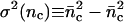 and σ²(n_e)) during two different time intervals (δt)

δt (s)
1.0	3.2	68.5	0.30	0.28
2.0	6.3	133.0	0.60	0.54

Fig. 3 shows the distribution of the encounter size s_e, averaged over 150 trajectories for L = 25 and We use 150 trajectories for the other calculated averages as well. From Fig. 3, we can see that the distribution looks reasonably geometric, as expected. We analyze the statistics of an encounter as follows. The first collision plays the role of the seed of the encounter, and it induces the next collision in the same encounter with a probability p_nc, where nc means next collision. Similarly, the second induces the third, etc., and at each stage the encounter can end with a probability of 1–p_nc. Thus the probability that s_e = n is and the average encounter size is As a first-order approximation, we use one value of p_nc for all encounters in Fig. 3. We obtain p_nc = 0.88 and by fitting the data in Fig. 3, but the value of obtained directly from the simulations is 10.7. We obtain a more refined estimate as follows. We evaluate the dependence of p_nc on the center-to-center z-direction displacement of the first collision of an encounter, which we call the encounter z-displacement (Δz_e), by dividing all encounters (2490) into two groups: group I for |Δz_e| < 150 Å (345) and group II for others (2145). Fitting gives p_nc = 0.93 and for group I, and p_nc = 0.871 and for group II. The overall average of is 8.8, closer to the value obtained directly. Thus, collisions with smaller Δz tend to induce larger encounters. Similarly, we study the dependence of p_nc on the filament-filament angle of the first collision of an encounter (θ_e). For the group with θ_e < 45° or θ_e > 135° (798 encounters), p_nc = 0.87 and ; for the group of the other encounters (1692), p_nc = 0.89 and Thus θ_e does not strongly affect p_nc.

FIGURE 3.

Distribution of the encounter size s_e. N(s_e) is the number of encounters with s_e collisions. (Solid line) Results from 150 trajectories for L = 25 and (Dotted line) Fit by the geometric distribution The geometric distribution is the discrete exponential distribution.

Flowchart for bundling

A typical simulation trajectory can be visualized according to the model shown in Fig. 4 a. It begins with the first free state (1F); the target filament collides with an environmental filament. Then it has three options: short free state (f), free state (F), and bundling (B). State f means the target filament will return to state c soon, in ≪0.1 s, whereas state F means the encounter ends and the target filament will return after at least 0.1 s. The probabilities from state c to states F, f, and B are p_cF, p_cf, and p_cB, respectively. The states labeled with lower-case letters are those with short lifetimes. We define the encounter state (E) in Fig. 4 b as the combination of states c and f. From our results, the time in state 1F is smaller but very close to that in state F. Thus we combine states 1F and F, and simplify the flow chart as in Fig. 4 c. In Fig. 4 c,

(10)

Here the t_F and t_E terms account for the time spent in states F and E, and the last term accounts for the probability that the filament is recycled to state F, starting the process over. So

(11)

where t_b is the bundling time, and t_X is the time in state X (X = c, f, F, 1F, E). Our results show that t_F and t_1F are much larger than t_c, t_f, and t_E. Therefore

(12)

FIGURE 4.

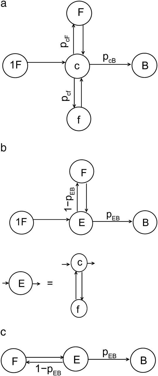
Flowchart of filament states. 1F, first free state; F, free state between two encounters; c, collision; E, encounter; f, short free state between two collisions; and B, bundling. (a) Flowchart for collisions; (b) flowchart for encounters; and (c) flowchart obtained by combining states 1F and F. Transition probabilities (p_cF, etc.) are defined in text.

Similarly, in Fig. 4 a, t_b = t_1F + (t_c + p_cft_f + p_cFt_F)/p_cB, and in Fig. 4 b, t_b = t_1F + (t_E + (1 − p_EB)t_F)/p_EB. Thus,

(13)

and

(14)

In Fig. 4 a, p_cf equals p_nc, because state f always induces the next collision in a very short time. In addition, p_cF + p_cf + p_cB = 1. Therefore,

(15)

and

(16)

Eqs. 15 and 16 define the relation between encounters and collisions.

Bundling probability of collision/encounters

We now consider the dependence of the bundling probability on the angle (θ_c or θ_e) and the center-to-center distance (d_cc) when the collision/encounter happens. Bundling is an orientationally constrained reaction. Therefore, the bundling probability p_cB of a collision, which is the probability that bundling occurs before the collision ends, is sensitive to the collision angle if E_mm is not extremely large. If E_mm is extremely large, every collision leads to bundling and p_cB = 1. We find that the distribution of collision angles (θ_c) is proportional to sin(θ_c), as expected. The collisions near θ_c = 90° are thus the most abundant. The solid line of Fig. 5 a shows the dependence of p_cB on θ_c for L = 25 and Collisions of smaller angle (those near 180° are equivalent to angles near 0°) have larger bundling probability. The most abundant collisions near θ_c = 90° have nearly zero bundling probability. But the situation is quite different for encounters. The encounter angle θ_e has no significant effect on p_b. The encounters near θ_e = 90° can lead to bundling, because the first collision of such an encounter can induce a collision of smaller angle and thus a larger bundling probability. As expected, the bundling probability of an encounter is much larger than that of a collision. Increasing the attraction increases the bundling probability and widens the range of collision angles that allow bundling (Fig. 5 b). The dot-dashed line for strong attraction is much more bumpy, because a bundling event includes much fewer collisions. Thus the total number of collisions is much less than those of the other two cases, and the sampling is insufficient. Similarly, curves for encounters are more bumpy than the corresponding ones for collisions in Fig. 5, a and c.

FIGURE 5.

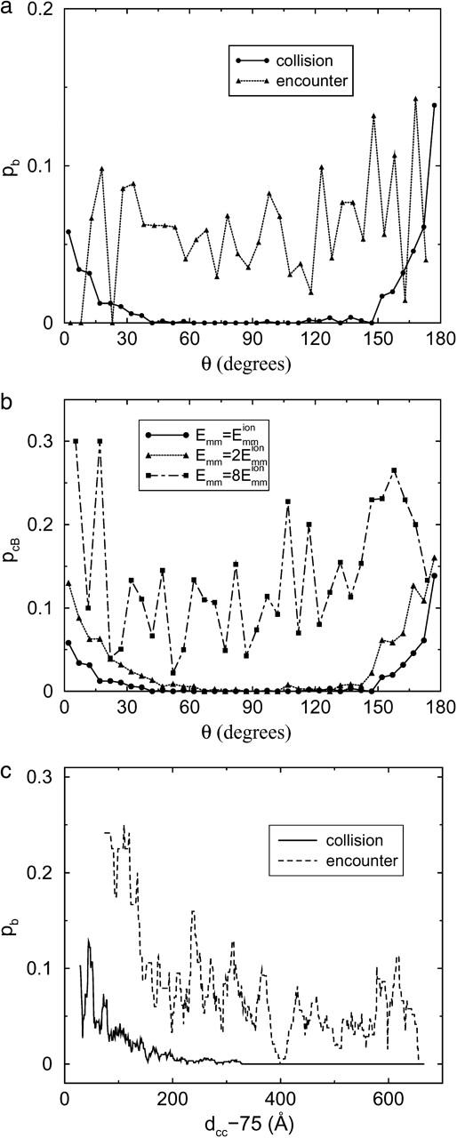
Dependence of bundling probability on filament geometry when collision/encounter begins. The value p_b is the probability that bundling happens in a given collision/encounter (p_cB or p_EB). The value θ is the angle between two filaments when they begin to collide. (a) Dependence of p_b on θ. (b) Dependence of p_cB on θ and the maximal attractive energy E_mm of two monomers. (c) Dependence of p_b on the center-to-center distance d_cc of two filaments. L = 25 for a–c and for all unlabeled curves.

Fig. 5 c shows that collisions/encounters with smaller d_cc tend to have larger bundling probabilities. Compared with the encounter angle, d_cc has a much stronger effect on p_EB. This is due to its effect on the encounter size. p_cB is also enhanced by smaller d_cc because the geometry is closer to the final bundled geometry. We extract the encounters with d_cc < 200 Å, and we find that their averaged size is 13.7, which is significantly larger than the global average of 10.7. Then we extract the encounters of θ < 45°, and find an average size of 10.5, very close to the global average 10.7. The encounter d_cc thus affects the encounter size and therefore the bundling probability, whereas the encounter angle does not.

Bundling process

The bundling process is seen most clearly in the case of strong attraction (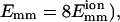 shown in Fig. 6 and the movie as supplemental material. Stronger attraction increases the duration of a collision, so it can induce more changes in the filaments' relative position and orientation. In Fig. 6 a, the energy fluctuates randomly before t = 7.2 μs; then it steeply drops to −1.2 eV and finally it drops more slowly, with fluctuations. In Fig. 6 b, θ also fluctuates before t = 7.2 μs; then it quickly drops to near 0° and stays there. The situation for the z-displacement Δz is similar to that for θ. However, the drop in Δz occurs later than the drop in θ. It fluctuates until E = −1.2 eV and then drops to zero (bundled state). These results clearly show that there are two phases: rotation and sliding. The initial rotation appears to be random. When θ reaches a certain limit, two filaments quickly align parallel to each other, and the energy drops steeply. Then the sliding begins and leads to bundling.

FIGURE 6.

Bundling for strong attraction and L = 25 . (a) Energy during last collision, which leads to bundling. The value t = 0 is the beginning time for this collision. (b) Angle θ (solid line) and displacement Δz along the z axis between the centers of two filaments (dotted line) during the last collision. Downward arrows mark separation of the rotation and sliding phases of bundling.

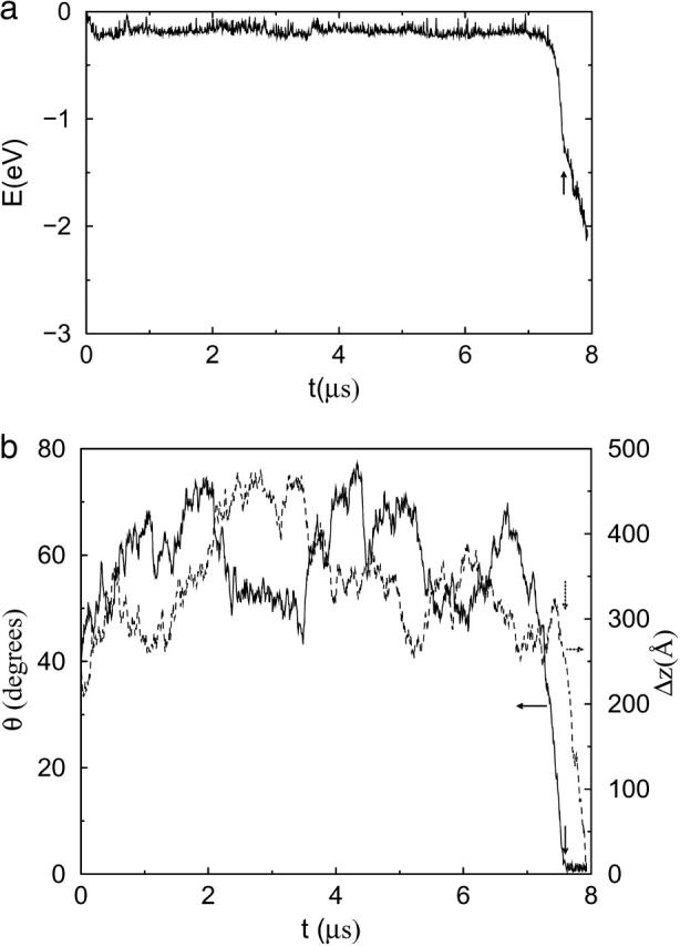
For weak attraction, a collision lasts a short time, and the driving force for rotation is weak, so only small geometric changes occur during a collision. Therefore, a high bundling probability for a collision requires small geometric differences in the collision angle and d_cc, as shown previously in Fig. 5. In Fig. 7, we show the final encounter of a typical such trajectory. Compared with Fig. 6 b which has θ = 40° and Δz = 245 Å, the final collision, which leads to bundling, has smaller values: θ = 8° and Δz = 20 Å. Many collisions are required to obtain a small-angle collision so that the filaments can bundle.

FIGURE 7.

Bundling for weak attraction and L = 25 . Energy (a), angle θ (b, solid line), and z-displacement Δz (b, dotted line) during last encounter. (Open triangles) Collisions begin; (solid circles) collisions end. Last collision leads to bundling.

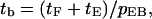
Bundling time

The bundling time depends on the attractive interaction, the filament length, and the diffusion coefficients, which are in turn determined by the filament geometry (length and radius) and the solution viscosity. In addition to performing simulations with the correct parameters, we also artificially change a single parameter at a time to evaluate its role in bundling. In our simulations, most of the trajectories, including almost all of those with the correct parameters, end in a bundled state, but some of the artificial simulations, especially those of extremely small D_r, do not always end with bundling within the time limit of our simulations. We obtain the bundling time t_b by dividing the total running time of all trajectories by the number of bundling trajectories (N_b): This is equivalent to assuming that those trajectories which do not bundle, on average, need an extra time t_b to bundle, i.e.,

The model given in Fig. 4 can help us analyze the bundling time. There are two timescales in a trajectory: the encounter timescale and the collision timescale. The trajectory consists of encounters and an encounter consists of collisions. We then define the trajectory size s_t as the number of encounters in a trajectory, and s_t should obey the geometric distribution according to the previous analysis of s_e. In addition, the distribution of the time in state F, t_F, obeys a continuous geometric (or exponential) distribution. For the 150 trajectories for L = 25 and the average t_F is 16.2 s and the standard deviation is 15.4 s; for an exactly exponential distribution, their values would be identical. In Fig. 4, the time in state E can be ignored in comparison with t_F according to our results, so

(17)

where t_Fi is the i^th t_F in a given trajectory. Thus the distribution of bundling times of a set of trajectories should be a geometric distribution. The average bundling time of the 150 trajectories for L = 25 and is 55.9 s and the standard deviation is 55.1 s, close to the average. This property strongly suggests an exponential distribution, which is confirmed by fitting the distribution. The error of the bundling time of one trajectory is exactly the real average bundling time Thus the error of the average bundling time of N_traj trajectories is i.e., the relative error is We keep N_traj ≥ 150, so relative errors are within 8%.

Fig. 8 shows the dependence of bundling time (Fig. 8 a) and its corresponding rate constant (Fig. 8 b) on attraction strength and filament length. In Fig. 8 a, increasing the attraction between the filaments decreases the bundling time. There is a diffusion limit for the bundling time. If the attraction is strong enough, p_EB = 1 and t_b = t_F according to Eq. 12; t_F is determined entirely by the diffusion coefficients and the filament length. The dependence of t_b on filament length (L) is weak. Although increasing the filament length can expand the capture region and thus decrease t_F and increase s_e, it also decreases the diffusion coefficients, which increases t_F. If the translational diffusion coefficients D_h and D_v changed by the same factor as the rotational diffusion coefficient D_r, adjusting the time step Δt by the inverse of this factor would leave Eqs. 6–10 unchanged and the bundling probability for a collision (p_cB) would be the same. But increasing L decreases D_r more than D_h and D_v, by a factor of L⁻². This results in a decrease of p_cB because p_cB is determined by the competition between rotation (dominated by D_r) and escape (controlled mainly by D_v and affected less by D_r and D_h). Because (Eq. 15), the dependence of p_EB on L is also determined by the same two competing factors as that of t_F on L. Therefore, t_b ∼ t_F/p_EB is only weakly affected by L. The dependences of the bundling parameters on L at are shown in Table 2. The dependences are weak, as expected. We also see t_1F ∼ t_F, supporting our earlier analysis.

FIGURE 8.

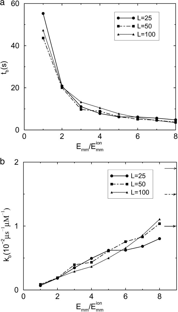
Dependence of bundling time t_b (a) and its corresponding rate constant k_b (b) on filament length and attraction. Increasing potential decreases the bundling time. Large D_r and E_mm give upper limits for bundling rate constants, whose values for the three lengths are marked by arrows in b.

TABLE 2.

Dependence of bundling parameters on L for

L	se	1/pcB	1/pEB	tF (s)	t1F (s)	tb (s)
25	10.7	178	16.7	3.33	2.91	55.3
50	17.9	285	15.9	2.73	2.80	43.6
100	33.5	702	20.9	2.27	2.19	47.3

s_e, average number of collisions in an encounter; 1/p_cB, average number of collisions needed for bundling; 1/p_EB, average number of encounters needed for bundling; t_F, average time in state F; t_1F, average time in state 1F; and t_b, average bundling time.

Increasing D_r should increase p_EB by increasing the orientational search speed, and decrease t_F by increasing the collision rate. Therefore, increasing D_r should decrease the bundling time t_b. This expectation is confirmed by the numerical results for the dependence of t_b, t_F, and p_EB on D_r, shown in Table 3. The inverse of p_EB is the number of encounters needed for bundling, which decreases with increasing D_r. This effect is stronger than the decrease in t_F.

TABLE 3.

Dependence of bundling time t_b, bundling probability p_EB of an encounter and time t_F in state F on D_r for L = 25 and

Dr	tF (s)	1/pEB	tb (s)
0.01	4.95	135	686
0.03	4.61	77.3	443
0.1	4.26	41.5	178
0.3	3.85	25.2	97
1	3.32	16.5	55
3	2.91	12.9	35
10	2.53	11.7	29

We vary D_r artificially while keeping other parameters fixed. Units of D_r are chosen such that original value is 1.

If D_r and E_mm are large enough, the two filaments will contact and bundle almost as soon as d_cc = L_f, since the orientational search will be faster than the translational search. We use a simple model to estimate the bundling rate constant in this limit. In this model, an environmental filament is centered in a sphere of radius R_s ≫ L_f and the target filament is randomly located at r (r < R_s). When d_cc = L_f, the target is captured. When the target is captured, bundling is almost instantaneous, so t_b is the capture time w(r). If the target moves out of the sphere, it is assumed to run into another sphere, so Therefore, according to Gardiner (1985),

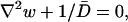(18)

with

where 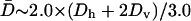is twice the average translational diffusion coefficient (twice because of the relative motion). The solution is

(19)

The average of w(r) shows that the last term dominates, i.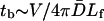e., where is the volume of the sphere. So the bundling rate constant k_b for large D_r and E_mm is The values for L = 25, 50, and 100 are 1.0 × 10⁻², 1.5 × 10⁻², and 1.9 × 10⁻² μM⁻¹ μs⁻¹, which are marked as arrows in Fig. 8 b. These limits are consistent with the numerical results. Because the effect of the reduced D_r coming from increasing L is ignored in the limits, the dependence of k_b on L is stronger than that in the numerical results, but still weak.

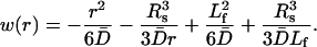
Two-step potential well model

To explain the dependence of t_b on E_mm, we use the two-step potential well model shown in Fig. 9 a. Particles reaching x = 0 are regarded as bundled and the particles are restricted to the region x ≤ X_c. The first well of depth −E₁ represents the rotation phase, and the second well, of depth −E₂ relative to the bottom of the first well, represents the sliding phase. When two filaments collide, the particle enters the first well; when they rotate and align parallel with each other, the particle drops into the second well. The first well thus shuttles the particle to the second well. The capture time for the particle at x, w(x), satisfies Gardner (1985),

(20)

with

where β is inverse temperature, is the force, and D is the diffusion coefficient. Letting u(x) ≡ Dw(x),

(21)

with

FIGURE 9.

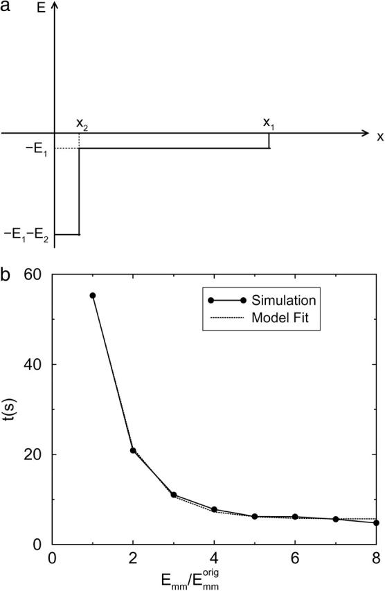
Two-step potential well model (a) and fitting results (b) for L = 25 using Eq. 25. The fit parameters are t_∞ = 5.68 s, t₀ = 162.2 s, and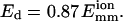

The solution for x > x₁ is

(22)

where u(x;a, b) is the solution for E₁ = a and E₂ = b (a and b can be 0 or ∞ here). The u functions in Eq. 22 are easily obtained, but we do not specify them here because they are not needed for our result.

Usually, the second well is much deeper and narrower than the first, and two filaments in the sliding phase almost always bundle (βE₂ ≫ 1). The first two terms can thus be ignored. So

(23)

and the bundling time

(24)

where t_∞ is the bundling time for E₁ = ∞ and t₀ is for E₁ = 0. We can assume that E₁ is proportional to E_mm, i.e., βE₂ = E_mm/E_d, where E_d is a constant, and

(25)

Thus dependence on E_mm is exponential. From Fig. 9 b, we can see that Eq. 25 fits the simulation results closely.

CONCLUSIONS

In summary, we have found the following. In a bundling event, collisions are clustered in time. Collisions of smaller angles and smaller d_cc are more likely to lead to bundling. The bundling process consists of two phases: rotating and sliding. The bundling rate depends only weakly on filament length. Increasing the attraction decreases the bundling time to a lower limit, which is determined by diffusion properties. A simple two-step-well model predicts an exponential dependence of the bundling time on the interaction strength, which is confirmed by the simulation results.

APPENDIX: COLLISION CLUSTERING

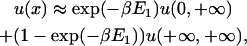
In this Appendix, we show, by studying a simple system, that the phenomenon of collision clustering (Northup and Erickson, 1992) is a universal and a direct property of random walks. In this system, two noninteracting particles are restricted to a one-dimensional lattice of unit spacing ranging from −X_m to X_m, where one is fixed at the center x = 0, and the other moves randomly. When the free particle meets the fixed one, a collision is counted. The free particle is reflected at the boundaries. The initial position of the free particle is randomly chosen. Fig. 10 shows a typical simulation trajectory for X_m = 100. Although there is no interaction between the two particles, collision clustering is obvious in Fig. 10 a, which shows the times of the first 200 sequential collisions.

FIGURE 10.

(a) Number of collisions n_c before time t, in which solid triangles show times of the first 200 sequential collisions in a simulation trajectory with X_m = 100 and 10⁹ steps; (b) probability distribution P(t_cc) of t_cc, the time spacing between two successive collisions, in the same simulation trajectory. Note that probability of odd t_cc is zero. For large, even t_cc values, the probabilities are close to zero, but are not zero. Probabilities of t_cc values >60 steps are not shown. Open triangles in b are probability ratios.

From this simulation trajectory, we obtain the distribution of time spacings t_cc between two successive collisions in Fig. 10 b. The t_cc distribution can be also calculated by the following method. First, we find all paths, from x = 0 to x = 0, of length t_cc; then we sum up the probabilities of these paths and obtain the probability of t_cc. For a path, the free particle at each point except the ending point and the boundary points can have two choices, so the probability of this path is 2⁻ⁿ, where n is the number of these points. As an example, for t_cc = 2, there are two paths: 0 → 1 → 0 (2⁻²) and 0 → −1 → 0 (2⁻²), where the numbers in parentheses are the corresponding probabilities. Thus, the probability of t_cc = 2 is 1/2. Similarly, for t_cc = 4, 6, 8, and 10, the probabilities are 1/8, 1/16, 5/128, and 7/256, respectively. These values are consistent with the simulation data in frame b. This distribution has two features. First, most of the probability is concentrated at small t_cc values, and the probability decreases with increasing t_cc. Thus, two successive collisions tend to cluster with small t_cc values. Second, the decrease slows down quickly with increasing t_cc, which is shown by the ratios of P(t_cc) to P(t_cc−2) in Fig. 10 b. Thus, there are still substantial probabilities for large t_cc values. For instance, there is a t_cc of ∼10,000 steps in Fig. 10 a. This feature guarantees that two successive collision clusters can be separated by large t_cc values, with a substantial probability. Collision clustering naturally results from these two properties.

References

- Baeza, I., P. Garislio, L. M. Rangel, P. Chavez, L. Cervants, C. Arguello, C. Wong, and C. Montanez. 1987. Electron microscopy and biochemical properties of polyamines-compacted DNA. Biochemistry. 26:6387–6392. [DOI] [PubMed] [Google Scholar]
- Bloomfield, V. A. 1996. DNA condensation by multivalent cations. Curr. Opin. Struct. Biol. 6:334–341. [DOI] [PubMed] [Google Scholar]
- Bloomfield, V. A. 1997. Polyelectrolyte effects in DNA condensation by polyamines. Biophys. Chem. 11:339–343. [DOI] [PubMed] [Google Scholar]
- Deserno, M., and C. Holm. 2002. Theory and simulations of rigid polyelectrolytes. Mol. Phys. 100:2941–2956. [Google Scholar]
- Diehl, A., H. A. Carmona, and Y. Levin. 2001. Counterion correlations and attraction between like-charged macromolecules. Phys. Rev. E. 64:011804-1–011804-6. [DOI] [PubMed] [Google Scholar]
- Doi, M., and S. F. Edwards. 1986. The Theory of Polymer Dynamics. Oxford University Press, New York. Chap. 8.
- Gardiner, C. W. 1985. Handbook of Stochastic Methods for Physics, Chemistry, and the Natural Sciences. Springer-Verlag, New York. Chap. 5.
- Gelbart, W. M., R. F. Bruinsma, P. A. Pincus, and V. A. Parsegian. 2000. DNA-inspired electrostatics. Phys. Today. 53:38–44. [Google Scholar]
- Grønbech-Jensen, N., R. J. Mashl, R. F. Bruinsma, and W. M. Gelbart. 1997. Counterion-induced attraction between rigid polyelectrolytes. Phys. Rev. Lett. 78:2477–2480. [Google Scholar]
- Ha, B.-Y., and A. J. Liu. 1997. Counterion-mediated attraction between two like-charged rods. Phys. Rev. Lett. 79:1289–1292. [Google Scholar]
- Kawamura, M., and K. Maruyama. 1970. Polymorphism of F-actin. I. Three forms of paracrystals. J. Biochem. (Tokyo). 68:885–899. [DOI] [PubMed] [Google Scholar]
- Khokhlov, A. R., and A. N. Semenov. 1985. On the theory of liquid-crystalline ordering of polymer chains with limited flexibility. J. Stat. Phys. 38:161–182. [Google Scholar]
- Kornyshev, A. A., and S. Leikin. 1998. Electrostatic interaction between helical macromolecules in dense aggregates: an impetus for DNA poly- and meso-morphism. Proc. Natl. Acad. Sci. USA. 95:13579–13584. [DOI] [PMC free article] [PubMed] [Google Scholar]
- Lau, A. W. C., and P. Pincus. 2002. Counterion condensation and fluctuation-induced attraction. Phys. Rev. E. 66:041501-1–041501-14. [DOI] [PubMed] [Google Scholar]
- Manning, G. S. 2003. Comments on selected aspects of nucleic acid electrostatics. Biopolymers. 69:137–143. [DOI] [PubMed] [Google Scholar]
- Moreira, A. G., and R. R. Netz. 2001. Binding of similarly charged plates with counterions only. Phys. Rev. Lett. 87:078301-1–078301-4. [DOI] [PubMed] [Google Scholar]
- Northrup, S. H., and H. P. Erickson. 1992. Kinetics of protein-protein association explained by Brownian dynamics computer simulation. Proc. Natl. Acad. Sci. USA. 89:3338–3342. [DOI] [PMC free article] [PubMed] [Google Scholar]
- Oosawa, F. 1968. Interaction between parallel rodlike macroions. Biopolymers. 5:1633–1647. [Google Scholar]
- Ray, J., and G. S. Manning. 1994. An attractive force between two rodlike polyions mediated by sharing of condensed counterions. Langmuir. 10:2450–2461. [Google Scholar]
- Rochet, J. C., and P. T. Lansbury. 2000. Amyloid fibrillogenesis: themes and variations. Curr. Opin. Struct. Biol. 10:60–68. [DOI] [PubMed] [Google Scholar]
- Schlosshauer, M., and D. Baker. 2002. A general expression for bimolecular association rates with orientational constraints. J. Phys. Chem. B. 106:12079–12083. [Google Scholar]
- Schmitz, K. S., and J. M. Schurr. 1972. Role of orientation constraints and rotational diffusion in bimolecular solution kinetics. J. Phys. Chem. 76:534–545. [Google Scholar]
- Sear, R. P. 1997. Cohesion and aggregation of flexible hard rods with an attractive interaction. Phys. Rev. E. 55:5820–5824. [Google Scholar]
- Shklovskii, B. I. 1999. Screening of a macroion by multivalent ions: correlation-induced inversion of charge. Phys. Rev. E. 60:5802–5811. [DOI] [PubMed] [Google Scholar]
- Shoup, D., G. Lipari, and A. Szabo. 1981. Diffusion-controlled bimolecular reaction rates. The effect of rotational diffusion and orientation constraints. Biophys. J. 36:697–714. [DOI] [PMC free article] [PubMed] [Google Scholar]
- Šolc, K., and W. H. Stockmayer. 1971. Kinetics of diffusion-controlled reaction between chemically asymmetric molecules. I. General theory. J. Chem. Phys. 54:2981–2988. [Google Scholar]
- Šolc, K., and W. H. Stockmayer. 1973. Kinetics of diffusion-controlled reaction between chemically asymmetric molecules. II. Approximate steady-state solution. Int. J. Chem. Kinet. 5:733–752. [Google Scholar]
- Stevens, M. J. 2001. Simple simulations of DNA condensation. Biophys. J. 80:130–139. [DOI] [PMC free article] [PubMed] [Google Scholar]
- Tang, J. X., and P. A. Janmey. 1996. The polyelectrolyte nature of F-actin and the mechanism of actin bundle formation. J. Biol. Chem. 271:8556–8563. [DOI] [PubMed] [Google Scholar]
- Tang, J. X., S. Wong, P. T. Tran, and P. A. Janmey. 1996. Counterion induced bundle formation of rodlike polyelectrolytes. Ber. Bunsenges. Phys. Chem. 100:796–806. [Google Scholar]
- van der Schoot, P., and T. Odijk. 1992. Statistical theory and structure factor of a semidilute solution of rodlike macromolecules interacting by van der Waals forces. J. Chem. Phys. 97:515–524. [Google Scholar]
- Yu, X. P., and A. E. Carlsson. 2003. Multiscale study of counterion-induced attraction and bundle formation of F-actin using an Ising-like mean field model. Biophys. J. 85:3532–3543. [DOI] [PMC free article] [PubMed] [Google Scholar]
- Zhou, H.-X. 1993. Brownian dynamics study of the influences of electrostatic interaction and diffusion on protein-protein association kinetics. Biophys. J. 64:1711–1726. [DOI] [PMC free article] [PubMed] [Google Scholar]
Associated Data
This section collects any data citations, data availability statements, or supplementary materials included in this article.