

Abstract
Amyloid fibrils are the structural components underlying the intra- and extracellular protein deposits that are associated with a variety of human diseases, including Alzheimer's, Parkinson's, and the prion diseases. In this work, we examine the thermodynamics of fibril formation using our newly-developed off-lattice intermediate-resolution protein model, PRIME. The model is simple enough to allow the treatment of large multichain systems while maintaining a fairly realistic description of protein dynamics when used in conjunction with constant-temperature discontinuous molecular dynamics, a fast alternative to conventional molecular dynamics. We conduct equilibrium simulations on systems containing 96 Ac-KA14K-NH2 peptides over a wide range of temperatures and peptide concentrations using the replica-exchange method. Based on measured values of the heat capacity, radius of gyration, and percentage of peptides that form the various structures, a phase diagram in the temperature-concentration plane is constructed delineating the regions where each structure is stable. There are four distinct single-phase regions: α-helices, fibrils, nonfibrillar β-sheets, and random coils; and four two-phase regions: random coils/nonfibrillar β-sheets, random coils/fibrils, fibrils/nonfibrillar β-sheets, and α-helices/nonfibrillar β-sheets. The α-helical region is at low temperature and low concentration. The nonfibrillar β-sheet region is at intermediate temperatures and low concentrations and expands to higher temperatures as concentration is increased. The fibril region occurs at intermediate temperatures and intermediate concentrations and expands to lower as the peptide concentration is increased. The random-coil region is at high temperatures and all concentrations; this region shifts to higher temperatures as the concentration is increased.
INTRODUCTION
Protein aggregation is a serious problem (Wetzel, 1994; King, 1989; Fink, 1998). It is a cause, or associated symptom, of over 20 different diseases including Alzheimer's (Kelly, 1998, 2002; Rochet and Lansbury, 2000; Dobson, 2001; Zerovnik, 2002); it can interfere with the recovery of recombinant proteins from inclusion bodies; and it is a nuisance in protein-folding experiments (Wetzel, 1994; King, 1989; Fink, 1998). The objective of the work presented in this article is to provide a general description of the dependence of protein aggregation on concentration and temperature. The focus is on ordered aggregates, e.g., amyloid or fibrils, rather than disordered aggregates, since these are the structures most often found in disease. Despite the numerous experimental investigations of amyloid formation appearing in the literature, little discussion of the sensitivity of amyloid formation to solution conditions, particular protein concentration, and temperature, has appeared. Although there have been two simulation-based investigations (Dima and Thirumalai, 2002; Jang et al., 2004b) that yield protein aggregation phase diagrams, the models studied are not realistic enough to offer guidance to experimentalists in choosing the concentration and temperature at which to conduct in vitro fibrillization experiments, or to avoid fibrillization. Here we present a computer simulation study of the phase change behavior of a model system of polyalanine peptides using a novel protein model, PRIME, that contains genuine protein-like character. Polyalanine was chosen for study because it is the simplest peptide known to form fibrils and because the basic physics underlying the fibrillization process is thought to be relatively independent of the peptide sequence. Equilibrium simulations are conducted on a 96-peptide system via the replica-exchange simulation method, leading to the construction of a phase diagram in the temperature-concentration plane delineating the regions where random coils, α-helices, β-sheets, fibrils, and other aggregates are stable.
Most simulation studies to date of fibril-forming peptides by other investigators have been limited to the study of either isolated peptides (Ilangovan and Ramamoorthy, 1998; Kortvelyesi et al., 2001; Massi et al., 2001, 2002; Massi and Straub, 2001a,b; Yang et al., 2003; Straub et al., 2002; Moraitakis and Goodfellow, 2003) or model amyloid fibrils that have already formed (Li et al., 1999; George and Howlett, 1999; Ma and Nussinov, 2002a,b; Lakdawala et al., 2002; Zanuy et al., 2003; Zanuy and Nussinov, 2003; Hwang et al., 2003). These studies have employed high-resolution protein models, which are based on a realistic representation of protein geometry and a fairly faithful accounting for the energetics of every atom on the protein and on the solvent. Although there have been several attempts (Mager, 1998a,b; Mager et al., 2001; Fernandez and Boland, 2002; Gsponer et al., 2003) using high-resolution protein models to simulate the formation of fibrils from random coils, the systems considered did not contain enough peptides to mimic the nucleus that stabilizes the large fibrils observed in experiments. Given current computational capabilities, simpler models are required. This has been recognized by a few investigators who have combined intermediate-resolution protein models with Gō potentials to look at fibril formation. Such an approach has been taken by Jang et al. (2004a,b), who studied the thermodynamics and kinetics of the assembly of four model β-sheet peptides into a tetrameric β-sheet complex, and by Ding et al. (2002), who studied the formation of a fibrillar double β-sheet structure containing eight model Src SH3 domain proteins. However, since the Gō potential contains a built-in bias toward the native conformation, this approach is not suitable for the study of spontaneous fibril formation from random configurations.
We take an alternative approach, which allows the treatment of large multichain systems while maintaining a fairly realistic description of protein dynamics without built-in bias toward any conformation. By combining an intermediate resolution protein model (described below) with discontinuous molecular dynamics simulation (Nguyen and Hall, 2004), we have been able to simulate the formation of fibrils by systems containing between 12 and 96 16-residue Ac-KA14K-NH2 peptides starting from the random-coil state. Our model is called PRIME; it was originally developed by Smith and Hall (2001a,b,c) and later improved by Nguyen et al. (2004). PRIME represents each amino acid with four beads—three for the backbone and one for the side chain. It is designed to be used with discontinuous molecular dynamics (DMD) (Alder and Wainwright, 1959; Rapaport, 1978, 1979; Bellemans et al., 1980), which is an extremely fast alternative to traditional molecular dynamics. DMD is applicable to systems of molecules interacting via discontinuous potentials, e.g., hard-sphere and square-well potentials. Solvent is modeled implicitly by including hydrophobic interactions between nonpolar side chains. Backbone hydrogen bonding is modeled in explicit detail. Using this algorithm, we (Nguyen and Hall, 2004) were able to sample much wider regions of conformational space, longer timescales, and larger systems than in traditional molecular dynamics. All simulations were performed in the canonical ensemble starting from a random-coil configuration equilibrated at a high temperature and then slowly cooled to the temperature of interest. Since the runs took only days on a workstation, we were able to conduct simulations at a wide variety of concentrations and temperatures, and to learn how peptide concentration and temperature affect the formation of various Ac-KA14K-NH2 structures including amorphous aggregates, α-helices, β-sheets, and fibrils. Although kinetic trapping in local free energy minima was minimized by slowly cooling a system that was initially at a high temperature down to the temperature of interest, we could never be certain if the system had reached equilibrium or gotten stuck in a metastable state.
In this article, we perform equilibrium simulations on 96-peptide systems over a very wide range of temperatures and peptide concentrations using the replica-exchange simulation method as originally formulated by Sugita and Okamoto (1999), who combined molecular dynamics and Monte Carlo (MD/MC) for simulations of protein folding. In this method, a number of replicas of the system are simulated at a spectrum of temperatures, usually on a system of parallel computers. At set time intervals, replicas whose temperatures are nearest-neighbors along the temperature spectrum are exchanged, provided that a Metropolis criterion is satisfied. This procedure is repeated until all of the systems at different temperatures reach equilibrium. At equilibrium, data on the probability of being in various energy levels and states are collected and stored for use in calculating various thermodynamic averages such as the radius of gyration Rg, the specific heat CV, and the internal energy E to determine the phase transitions of the systems at different temperatures and concentrations. The results are summarized in a phase diagram in the temperature-concentration plane.
The model polyalanine peptide chosen for study is the peptide Ac-KA14K-NH2. We focus on polyalanine-based peptides for three reasons. First, the small, uncharged, unbranched nature of alanine residues is amenable to simulation with the intermediate-resolution protein model, PRIME, that we developed previously (Smith and Hall, 2001a,b). Second, polyalanine repeats have been implicated in human pathologies; in particular, they are responsible for the formation of anomalous filamentous intranuclear inclusions in patients having a disease called oculopharyngeal muscular dystrophy, which is characterized by having difficulty in swallowing, eyelid drooping, and limb weakness (Brais et al., 1999). Third, synthetic polyalanine-based peptides have been shown by Blondelle and co-workers to undergo a transition from α-helical structures to β-sheet complexes in vitro (Forood et al., 1995; Blondelle et al., 1997), mimicking the structural transition believed to be a prerequisite for fibril nucleation and growth (Kirschner et al., 1986; Simmons et al., 1994; Horwich and Weissman, 1997; Sunde and Blake, 1997; Kusumoto et al., 1998; Harrison et al., 1999; Esler et al., 2000). Blondelle and co-workers observed that the α-helical structures were stabilized in part by intramolecular α-helical bonds and that the macromolecular β-sheet complexes were stabilized by hydrophobic intersheet interactions. Using circular dichroism, Fourier-transform infrared spectroscopy, and reversed-phase high-performance liquid chromatography, they found that 1), β-sheet complex formation increased with increasing temperature, exhibiting an S-shaped dependence on temperature with a critical temperature of 45°C at a peptide concentration of 1.8 mM and an incubation time of 3 h; and 2), β-sheet complex formation increased with increasing peptide concentration above a critical concentration of 1 mM at 65°C.
Highlights of our simulation results are the following. There are four distinct single-phase regions in which α-helices, fibrils, β-sheets, and random coils are stable. There are four different two-phase regions: random coils/nonfibrillar β-sheets; random coils/fibrils; fibrils/nonfibrillar β-sheets; and α-helices/nonfibrillar β-sheets. The α-helical region is at low temperatures and low concentrations. The nonfibrillar β-sheet region is at intermediate temperatures and low concentrations and expands to higher temperatures as concentration is increased. The fibril region occurs at intermediate temperatures at intermediate concentrations and expands to lower temperatures as the peptide concentration is increased. The random-coil region is at high temperatures and all concentrations; it shifts to higher temperatures as the concentration is increased.
This article is organized as follows. The next section, Methods, describes the methods used in this work, including the protein's physical representation, its potential energy function, the DMD simulation technique, and the replica-exchange method. Results and Discussion presents the results obtained from simulations at various conditions. Conclusions contains a summary of our findings.
METHOD
Model peptide and forces
The model peptide is 16 residues long with the sequence PH14P, where H stands for a hydrophobic amino acid residue and P stands for a polar amino acid residue. This sequence was chosen to approximate Ac-KA14K-NH2 peptides which have been shown by Blondelle and co-workers (Forood et al., 1995; Blondelle et al., 1997) to form stable, soluble β-sheet complexes. The peptide is represented at an intermediate level of resolution using a model introduced by Smith and Hall (2001a,b,c), which we now call PRIME (Protein Intermediate-Resolution Model). Details of the model including values for all parameters are given in earlier articles (Smith and Hall, 2001a,b; Nguyen et al., 2004). The model is based on a four-bead amino acid representation with realistic bond lengths and bond-angle constraints and has the ability to interact both intra- and intermolecularly via hydrogen bonding and hydrophobic interaction potentials. The geometry of the protein model is illustrated in Fig. 1. Each amino acid residue is composed of four spheres—a three-sphere backbone comprised of united atom NH, CαH, and C=O, and a single bead side-chain R (these are labeled N, Cα, C, and R, respectively, in the figure). All backbone bond lengths and bond angles are fixed at their ideal values; the distance between consecutive Cα atoms is fixed so as to maintain the interpeptide bond in the trans configuration. The side chains are held in positions relative to the backbone such that all residues are L-isomers.
FIGURE 1.

Geometry of the intermediate-resolution protein model for polyalanine. Covalent bonds are shown with narrow solid lines connecting beads. At least one of each type of pseudobond is shown with a thick disjointed line. Pseudobonds are used to maintain backbone bond angles, consecutive Cα distances, and residue L-isomerization. Note that, for ease of viewing, the united atoms are not shown full size.
The solvent is modeled implicitly in the sense that its effect is factored into the energy function as a potential of mean forces. All forces are modeled by either hard-sphere or square-well potentials. The excluded volumes of the four united atoms are modeled using hard-sphere potentials with realistic diameters. Covalent bonds are maintained between adjacent spheres along the backbone by imposing hard-sphere repulsions whenever the bond lengths attempt to move outside of the range between l(1−δ) and l(1+δ) where l is the bond length and δ is a tolerance which we set equal to 2.375% (Nguyen et al., 2004). Ideal backbone bond angles, Cα–Cα distances, and residue L-isomerization are achieved by imposing pseudobonds, as shown in Fig. 1, which also fluctuate within a tolerance of 2.375%. Interactions between hydrophobic side chains are represented by a square-well potential of depth εHP and range 1.5 σR, where σR is the side-chain diameter. Hydrophobic side chains must be separated by at least three intervening residues to interact. Hydrogen bonding between amide hydrogen atoms and carbonyl oxygen atoms on the same or neighboring chains are represented by a square-well attraction of strength εHB between NH and C=O united atoms, whenever: 1), the virtual hydrogen and oxygen atoms (whose location can be calculated at any time) are separated by 4.2 Å (the sum of the NH and C=O well widths); 2), the nitrogen-hydrogen and carbon-oxygen vectors point toward each other within a fairly generous tolerance; 3), neither the NH nor the C=O is involved yet in a hydrogen bond with a different partner; and 4), the NH and C=O are separated by at least three intervening residues along the chain.
To satisfy the second requirement, the separations between the four auxiliary pairs, Ni–Cα,j, Ni–Nj+1, Cj–Cα,i, and Cj–Ci–1, surrounding the hydrogen bond in question, are limited to certain distances that are chosen to maintain ideal hydrogen bond angles. This is accomplished by imposing square-shoulder interactions between the auxiliary pairs as suggested in the work by Ding et al. (2003). Besides adding stability to the hydrogen bond, these interactions exact a penalty for breaking a hydrogen bond when any one of these auxiliary pairs moves inside the specified separation and thus distorts the hydrogen bond angle. For more details on the hydrogen bonding model used here, see a recent article by Nguyen et al. (2004). For simplicity, the strength of a hydrophobic contact, εHP, is fixed at 1/10 the strength of a hydrogen bond, εHB. Hydrogen bond strength and hydrophobic contact strength are independent of temperature, as has been assumed in previous simulation studies (Irback et al., 2000; Smith and Hall, 2001b,c).
Discontinuous molecular dynamics
Simulations are performed using the discontinuous molecular dynamics (DMD) simulation algorithm (Alder and Wainwright, 1959; Rapaport, 1978, 1979; Bellemans et al., 1980), which is an extremely fast alternative to traditional molecular dynamics and is applicable to systems of molecules interacting via discontinuous potentials, e.g., hard-sphere and square-well potentials. DMD simulations are conducted as follows. Each bead of the model protein chain is assigned a random initial position and a random initial velocity that do not violate any of the size constraints or assigned bond lengths and angles. The initial velocities are chosen at random from a Maxwell-Boltzmann distribution at a specified reduced temperature T* = kBT/εHB, where kB is Boltzmann's constant, T is temperature, and εHB is the strength of the hydrogen bond in the model as explained earlier. When a DMD simulation begins, each bead moves with its individual velocity. The simulation proceeds according to the following schedule: identify the first event (e.g., a collision), move forward in time until that event occurs, calculate new velocities for the pair of beads involved in the event and calculate any changes in system energy resulting from hydrogen bond events or hydrophobic interactions, find the second event, and so on. Types of events include excluded volume events, bond events, and square-well hydrogen bond and hydrophobic interaction events. An excluded volume event occurs when the surfaces of two hard-sphere beads collide and repel each other. A bond (or pseudobond) event occurs via a hard-sphere repulsion when two adjacent spheres attempt to move outside of their assigned bond length. Square-well events include well-capture, well-bounce, and well-dissociation “collisions” when a sphere enters, attempts to leave, or leaves the square well of another sphere. For more details on DMD simulations with square-well potentials, see articles by Alder and Wainwright (1959) and Smith et al. (1997).
Simulations are performed in the canonical ensemble which means that the number of particles, the volume, and the temperature are held constant. Periodic boundary conditions are used to eliminate artifacts due to simulation box walls. The dimensions of the box are chosen to ensure that a chain cannot interact with more than one image of any other chain. Constant temperature is achieved by implementing the Andersen thermostat method (Andersen, 1980) as was used previously (Zhou et al., 1997; Smith and Hall, 2001a). With this procedure, all beads in the simulation are subject to random collisions with ghost particles. The post-event velocity of a bead colliding with a ghost particle is chosen randomly from a Maxwell-Boltzmann distribution at the simulation temperature.
Replica-exchange DMD/MC method
The replica-exchange method is implemented in five 96-peptide simulations conducted at concentrations c = 0.5, 1.0, 2.0, 3.5, and 5.0 mM, which range from the very dilute regime, in which most peptides do not interact with neighboring peptides, to the highly concentrated regime, in which most peptides are in contact with neighboring peptides. At each concentration, the simulation contains 32 replica systems distributed over a broad interval of temperature ranging from T* = 0.09 to a high temperature at which each peptide is a random coil. Each replica system is simulated at a different temperature T in the canonical ensemble using the DMD method. The number of replicas and the distribution of temperatures are chosen to ensure that 1), there is a free random walk in temperature space, which means that every replica has the same probability of being switched to a neighboring temperature; 2), the number of replicas and hence temperatures sampled must be high enough to ensure that the probability of each replica being switched to a neighboring temperature is >10%; and 3), the highest temperature sampled must be high enough to prevent the system from becoming trapped in a local energy minimum. These requirements are the same as those stated by Sugita and Okamoto (1999).
At fixed time intervals, replicas are sorted from lowest to highest temperature and subjected to the following temperature MC exchange procedure. Systems i and j, with neighboring temperatures Ti and Tj, respectively, can exchange configurations (system i changes to temperature Ti and system j to temperature Tj) with the probability
 |
(1) |
where Δ = [βj–βi](Ui–Uj) with βi = 1/(kBTi) and Ui the potential energy of the system in state i. Initially each system is in a random configuration obtained from an NVT simulation at high temperature. Exchange attempts occur every t* = 0.5 reduced time units. The reduced time is  , with t the simulation time, and σ and m the average united atom diameter and mass. This corresponds to a replica-exchange attempt after ∼40,000,000 collisions at each temperature at low concentrations (c = 0.5 mM) or 60,000,000 collisions at each temperature at high concentrations (c = 5.0 mM). Approximately 1000 replica-exchange attempts are made during our simulations before equilibrium is reached. The criteria for equilibrium is that the ensemble average of the system's total potential energy, which is collected at the end of each DMD run, should vary by no more than 2.5% during the second half of all DMD runs at each temperature.
Once equilibrium is reached, the data collection phase begins in which 300 extra replica-exchange attempts are made. During the data collection phase, the properties of interest at each temperature are calculated throughout each DMD run. At the end of the replica-exchange DMD/MC simulation, our data contain a large ensemble of peptide configurations at each temperature and peptide concentration. Our simulations last more than 60,000,000,000 collisions at each temperature. A replica-exchange DMD/MC simulation at a single hydrophobic interaction strength and concentration requires 36 days on a cluster of 16 2.8-Ghz Xeon processors.
Our results are reported in part in terms of the average percentage of peptides in the system that form different structures. The structures of particular interest are α-helices, amorphous aggregates, fibrils, nonfibrillar β-sheets, β-hairpins, and random coils. They are defined in the following way. If 12 intrapeptide α-helical hydrogen bonds (defined as bonds between Ni+4 and Ci) are formed, the structure is an α-helix. If each peptide in a group of peptides has at least two interpeptide hydrogen bonds or hydrophobic interactions with a neighboring peptide in the same group, then that group is classified as an aggregate. Aggregates can be either ordered or amorphous. If an aggregate contains β-sheets or fibrils, we classify it as an ordered aggregate; otherwise, we classify it as an amorphous aggregate. If each peptide in a group of peptides has at least seven interpeptide β-hydrogen bonds to a particular neighboring peptide in the group, we classify this group as a β-sheet. (A β-hydrogen bond is a hydrogen bond between two residues whose backbone angles are in the β-region of the Ramachandran plot.) If at least two β-sheet structures form intersheet hydrophobic interactions (at least four hydrophobic interactions per peptide per β-sheet) and the β-sheet structures are at an angle <35°, we classify this as a fibril; otherwise, we classify this and isolated β-sheets as nonfibrillar β-sheet structures. A single-peptide β-structure such as a β-hairpin and a β-turn is defined as having three or more intrapeptide β-hydrogen bonds. Single-peptide structures that are not α-helices or β-structures but have a small number of intrapeptide hydrogen bonds or hydrophobic interactions are random coils.
To locate thermodynamic transitions, we determined the average radius of gyration Rg, the reduced specific heat  , and the potential energy E. The potential energy of the system E is the sum of the energy contributed by hydrogen bonds (the number of hydrogen bonds × εHB) and the energy contributed by hydrophobic interactions (the number of hydrophobic interactions × εHP). The reduced specific heat,
  , is calculated from the average potential energy 〈E〉 and the average squared potential energy 〈E2〉,
 |
(2) |
RESULTS AND DISCUSSION
Since this article builds upon our previous work (Nguyen and Hall, 2004) on the fibril formation of peptides of the same sequence, it is useful to briefly review those results that are pertinent to the discussion here. We investigated how peptide concentration and temperature affect the formation of various Ac-KA14K-NH2 structures including α-helices, β-sheets, and fibrils. By applying the discontinuous molecular dynamics simulation algorithm to our intermediate-resolution protein model, slow-cooling simulations were conducted on systems of 12, 24, 48, and 96 model 16-residue peptides at a wide variety of concentrations and temperatures. All simulations were performed in the canonical ensemble starting from a random-coil configuration equilibrated at a high temperature and then slowly cooled to the temperature of interest so as to minimize kinetic trapping in local free energy minima. Structural characteristics such as the peptide arrangement and packing within fibrils were examined and compared with those observed in experiments.
We were able to observe the formation of small fibrils (or protofilaments) containing 12–96 polyalanine peptides starting from random coils in a relatively short period of time ranging between 40 and 160 h on a single processor of an AMD Athlon MP 2200+ workstation. To our knowledge, these were the first simulations to span the whole process of fibril formation from the random-coil state to the fibril state on such a large system. We found that there was a strong relationship between the formation of α-helices, β-sheets, aggregates, and fibrils and the environmental conditions such as temperature, concentration, and hydrophobic interaction strength. The critical concentration for fibril formation increased with increasing temperature in qualitative agreement with the experimental results of Blondelle and co-workers on Ac-KA14K-NH2 peptides (Forood et al., 1995; Blondelle et al., 1997). The fibrils observed in our simulations mimicked the structural characteristics observed in experiments in that most of the peptides in our fibrils were arranged in an in-register parallel orientation, with intrasheet and intersheet distances similar to those observed in experiments, and contained approximately six multipeptide β-sheets. We also observed the formation of amorphous aggregates at intermediate concentrations (1.0 mM ≤ c < 5.0 mM) and at low temperatures (T* = 0.08–0.09). (Almost 20% of the peptides within these aggregates were in α-helical conformations.) Finally, we found that when the strength of the hydrophobic interaction between nonpolar side chains relative to the strength of hydrogen bonding was increased from R = 1/10 to R = 1/6, the system formed amorphous rather than fibrillar aggregates; this is reminiscent of the kinetic partitioning mechanism of Guo and Thirumalai (1996) in the simulations of protein folding using minimal models. We also identified key fibril-forming events. Since simulations were conducted by slowly cooling the system down to the temperature of interest, analysis of the temperature-dependence of the kinetics of fibril formation was not appropriate.
We then investigated the kinetics of fibril formation of Ac-KA14K-NH2 peptides as a function of the peptide concentration and temperature (Nguyen and Hall, 2004). Constant-temperature simulations were conducted on systems containing 48 model 16-residue peptides in the canonical ensemble at a wide variety of concentrations and temperatures. During each simulation, the formation of different structures such as α-helices, amorphous aggregates, β-sheets, or fibrils was monitored as a function of time. Key fibril-forming events were identified and compared with proposed fibril-formation mechanisms appearing in the literature. The lag time before fibril formation commences decreased with increasing concentration and increased with increasing temperature. In addition, the initial formation of a small fibril (or protofilament) appeared to undergo a process in which small amorphous aggregates→β-sheets→ordered nucleus→subsequent rapid growth of a stable fibril. Fibril growth in our simulations involved both β-sheet elongation, in which the fibril grows by adding individual peptides to the end of each β-sheet, and lateral addition, in which the fibril grows by adding already-formed β-sheets to its side. Once the fibrils attained a size of six sheets, they grew further through a β-sheet elongation mechanism. Moreover, the rate of fibril formation increased with increasing concentration and decreased with increasing temperature.
We now describe the results from equilibrium (replica-exchange) simulations of 96-peptide systems, the subject of this article.
Time-dependent structural transformation
Even though replica-exchange simulations are designed to sample structures and properties at equilibrium, it is of interest to consider how the various structures observed at different concentrations and temperatures evolve as the system heads toward equilibrium. At low concentrations, the structures observed over the course of the simulation at the various temperatures do not change with time (data not shown). For example, at c = 0.5 mM, the replicas at low temperatures initially form α-helices which remain stable throughout the whole simulation; likewise, the replicas at high temperatures form random coils throughout the whole simulation. In contrast, at intermediate concentrations, the structures initially formed by the replicas at low temperatures are different than the equilibrium structures observed much later in the simulation. This can be seen in Fig. 2, which plots the number of intramolecular α-helical hydrogen bonds and the number of intermolecular hydrogen bonds at c = 3.5 mM as a function of the number of replica-exchange attempts at different temperatures (T* = 0.09, 0.11, and 0.13). At the beginning of the simulation, the replicas at T* = 0.09 form a relatively high number of intramolecular α-helical hydrogen bonds and intermolecular hydrogen bonds, indicating a structure that is an amorphous aggregate with embedded α-helices as shown in Fig. 3 a. This amorphous structure is similar to those in our previous slow-cooling and constant-temperature simulations. Fig. 2 also indicates that the replicas at higher temperatures, T* = 0.11 and 0.13, initially form more intermolecular hydrogen bonds than those at T* = 0.09; these structures contain many β-sheets (not shown). As the simulation proceeds, the replicas at low temperatures are replaced by those at higher temperatures and the replicas at high temperatures are replaced by those at lower temperatures. After ∼150 replica-exchange attempts, the α-helix-containing amorphous aggregates that are formed at low temperatures have dissolved at the high temperature. In other words, at low temperatures, the peptides form intramolecular α-helical hydrogen bond contacts, which are the easiest to make and so form first. These α-helices are prone to aggregation once they gain the high kinetic energies from the elevated temperatures. They then modify their bonds and structure to form a more stable β-sheet aggregate structure. This can be seen in Fig. 2, which shows a decrease in the number of intramolecular α-helical hydrogen bonds and an increase in the number of intermolecular hydrogen bonds by 150 replica-exchange attempts. After 650 replica-exchange attempts, the dissolution of amorphous aggregates with α-helices is complete at low temperatures; the equilibrium structure is a fibril that contains several separate β-sheets as shown in Fig. 3 b. This indicates that the amorphous structures formed at intermediate concentrations and low temperatures in our previous slow-cooling and constant-temperature simulations were kinetically trapped in local minima.
FIGURE 2.

The number of intramolecular α-helical hydrogen bonds (solid lines) and the number of intermolecular hydrogen bonds (dashed lines) versus the number of replica-exchange attempts at concentration c = 3.5 mM and reduced temperatures (a) T* = 0.09, (b) T* = 0.11, and (c) T* = 0.13.
FIGURE 3.

Snapshots of a 96-peptide (a) amorphous aggregate obtained early and (b) fibrillar structure obtained at equilibrium from the c = 3.5 mM simulation at T* = 0.09. The amorphous aggregate contains α-helices that are shown in blue. The fibrillar structure is viewed down the fibril axis with hydrophobic side chains in red. Backbone atoms of different peptides have different colors, assigned so that it will be easy to distinguish the various sheets. Note that, for ease of viewing, the united atoms are not shown full size.
Structures at equilibrium
At low concentrations, as the temperature increases the system goes from a one-phase region containing α-helices to a narrow two-phase region containing both nonfibrillar β-sheets and random coils and then to a one-phase region containing random coils. This can be seen in Fig. 4, which plots the percentage of peptides in different structures as a function of the reduced temperature T* for the 96-peptide system at c = 0.5 mM. This figure indicates that at low temperatures (T* ≈ 0.09–0.11), the vast majority of peptides form α-helices as expected based on the intrinsic α-helical property of polyalanines in dilute solutions. The temperature at which half of the peptides form α-helices is T* = 0.11, which is the midpoint of the folding transition (50% helicity) of a single peptide from our previous simulations (Nguyen et al., 2004). As the temperature increases to intermediate temperatures (T* ≈ 0.110–0.135), the system goes to a two-phase region that has predominantly random coils and less prominently nonfibrillar β-sheets. The formation of β-structures at intermediate temperatures is also observed for single peptides based on our previous simulations (Nguyen et al., 2004). At high temperatures (T* > 0.135), the only structure that appears is the random coil.
FIGURE 4.

The percentage of peptides in α-helices (•), fibrils (□), nonfibrillar β-sheets (♦), amorphous aggregates (▵), hairpins (▴), and random coils (*) versus the reduced temperature T* for the 96-peptide system at c = 0.5 mM.
The existence of a transition between a one-phase region containing α-helices and a two-phase region containing both nonfibrillar β-sheets and random coils is supported by the data in Fig. 5, which plots the reduced specific heat  and radius of gyration Rg (in Å) as a function of the reduced temperature T* for the same system as in Fig. 4. The transition temperature can be identified from the peaks in the specific heat
  , which is the slope of the potential energy with respect to the temperature. The reduced specific heat
  data in Fig. 5 show the transition between a one-phase region containing α-helices and a two-phase region containing both nonfibrillar β-sheets and random coils at T* = 0.110, which is the same as the midpoint of the α-helical folding transition at T* = 0.110 deduced from Fig. 4. The radius of gyration also reflects the phase transition. For example, the radius of gyration in the one-phase region which contains α-helices (e.g., at T* = 0.09) is 7.31 Å, which is comparable to 7.27 Å for a perfect α-helix. In the two-phase region which contains both random coils and nonfibrillar β-sheets, the radius of gyration (e.g., at T* = 0.12) is 11.77 Å, which is between the value of 10.45 Å for a single random-coil conformation and 13.10 Å for an extended peptide conformation such as those observed in β-sheets in our previous simulation studies (Nguyen and Hall, 2004). In the one-phase random coil region at T* > 0.12, the radius of gyration (e.g., at T* = 0.14) is 11.41 Å, which is comparable to the value for a typical random coil.
FIGURE 5.

Reduced specific heat  and radius of gyration Rg (in Å) versus the reduced temperature T* for the 96-peptide system at c = 0.5 mM.
As the concentration increases from c = 0.5 mM to c = 1.0 mM, the transition between different phases is hard to detect since at each temperature the system contains more than one structural state as can be seen in Fig. 6, which plots the percentage of peptides in different structures as a function of the reduced temperature T* for the 96-peptide system at c = 1.0 mM. At low temperatures (T* < 0.095), the structural state that has the highest number of peptides is the α-helical structure at ∼40%, followed by the nonfibrillar β-sheet at ∼30% and the amorphous aggregates at ∼25%. As the temperature increases above T* = 0.095, the percentages of peptides that form α-helices and amorphous aggregates decrease. In contrast, the percentage of peptides that form nonfibrillar β-sheets increases to a maximum at T* = 0.115. Over the temperature range T* = 0.115–0.125, the percentage of peptides that form nonfibrillar β-sheets is relatively high with a peak of 60% at T* = 0.115; at that same temperature the percentage of peptides that form each of the other structures (fibrils, amorphous aggregates, and β-hairpins) is ∼10%. As the temperature increases from T* = 0.125 to T* = 0.14, the percentage of peptides that form fibrils increases, peaking at a value of 20%. Over this temperature range only 5% of the peptides form amorphous aggregates; the remaining 75% of the peptides form random coils.
FIGURE 6.

The percentage of peptides in α-helices (•), fibrils (□), nonfibrillar β-sheets (♦), amorphous aggregates (▵), hairpins (▴), and random coils (*) versus the reduced temperature T* for the 96-peptide system at c = 1.0 mM.
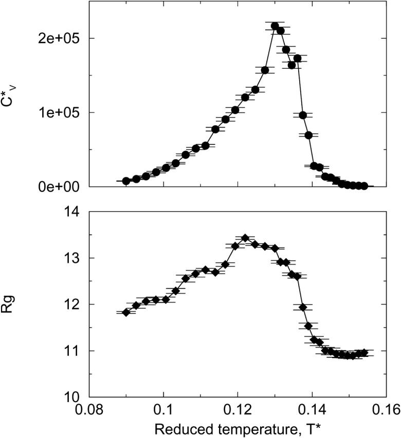
The thermodynamic properties  and Rg of the system at c = 1.0 mM are shown in Fig. 7, which plots the reduced specific heat
  and radius of gyration Rg (in Å) as a function of the reduced temperature T* for the same system as in Fig. 6. The specific heat results show a peak at ∼T* = 0.128; this corresponds to the midpoint of the nonfibrillar β-sheet curve reflecting a phase transition between a multiple-phase region in which nonfibrillar β-sheets are dominant and a multiple-phase region in which random coils are dominant. The radius of gyration results show more phase transitions than the specific heat data. At T* < 0.095, the radius of gyration is Rg = 8.5 Å, which is closer to the value for a perfect α-helix (7.27 Å) than to the random-coil-like value found in amorphous aggregates (10.45 Å), or the value in a β-sheet conformation (13.10 Å). At T* = 0.10–0.11, the radius of gyration increases to Rg = 11.0 Å, which is an average of the values for α-helices and β-sheets. The radius of gyration then increases to Rg = 12.5 Å at T* = 0.125, marking the region where the vast majority of peptides are nonfibrillar β-sheets. The radius of gyration then decreases to 11.0 Å at T* = 0.14 and beyond for the random coil.
FIGURE 7.
Reduced specific heat  and radius of gyration Rg (in Å) versus the reduced temperature T* for the 96-peptide system at c = 1.0 mM.
As the concentration increases from c = 1.0 mM to c = 2.0 mM, there is a transition between a two-phase region containing fibrils and nonfibrillar β-sheets and a one-phase region containing random coils as can be seen in Fig. 8, which plots the percentage of peptides in different structures as a function of the reduced temperature T* for the 96-peptide system at c = 2.0 mM. At T* < 0.14, most peptides are in β-sheets, both fibrillar and nonfibrillar. In addition, ∼10–20% of peptides are in amorphous aggregates. At T* ≥ 0.14, most peptides are random coils.
FIGURE 8.

The percentage of peptides in α-helices (•), fibrils (□), nonfibrillar β-sheets (♦), amorphous aggregates (▵), hairpins (▴), and random coils (*) versus the reduced temperature T* for the 96-peptide system at c = 2.0 mM.
The thermodynamic properties  and Rg of the system at c = 2.0 mM show the transition between the β-sheets and the random coil as seen in Fig. 9, which plots the reduced specific heat
  and radius of gyration Rg (in Å) as a function of the reduced temperature T* for the same system as in Fig. 8. The transition occurs at T* = 0.14.
FIGURE 9.
Reduced specific heat  and radius of gyration Rg (in Å) versus the reduced temperature T* for the 96-peptide system at c = 2.0 mM.
As the concentration increases from c = 2.0 mM to c = 3.5 mM, there is only one transition—between the fibrils and random coils—as can be seen in Fig. 10, which plots the percentage of peptides in different structures as a function of the reduced temperature T* for the 96-peptide system at c = 3.5 mM. At T* < 0.11, most peptides are in fibrils but some peptides are in nonfibrillar β-sheets. At T* = 0.11–0.13, the population of fibrils remains high. At T* > 0.13, the percentage of peptides that form fibrils decreases as the percentage of peptides that form random coils increases.
FIGURE 10.

The percentage of peptides in α-helices (•), fibrils (□), nonfibrillar β-sheets (♦), amorphous aggregates (▵), hairpins (▴), and random coils (*) versus the reduced temperature T* for the 96-peptide system at c = 3.5 mM.
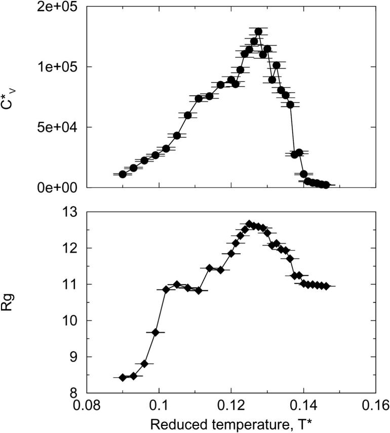
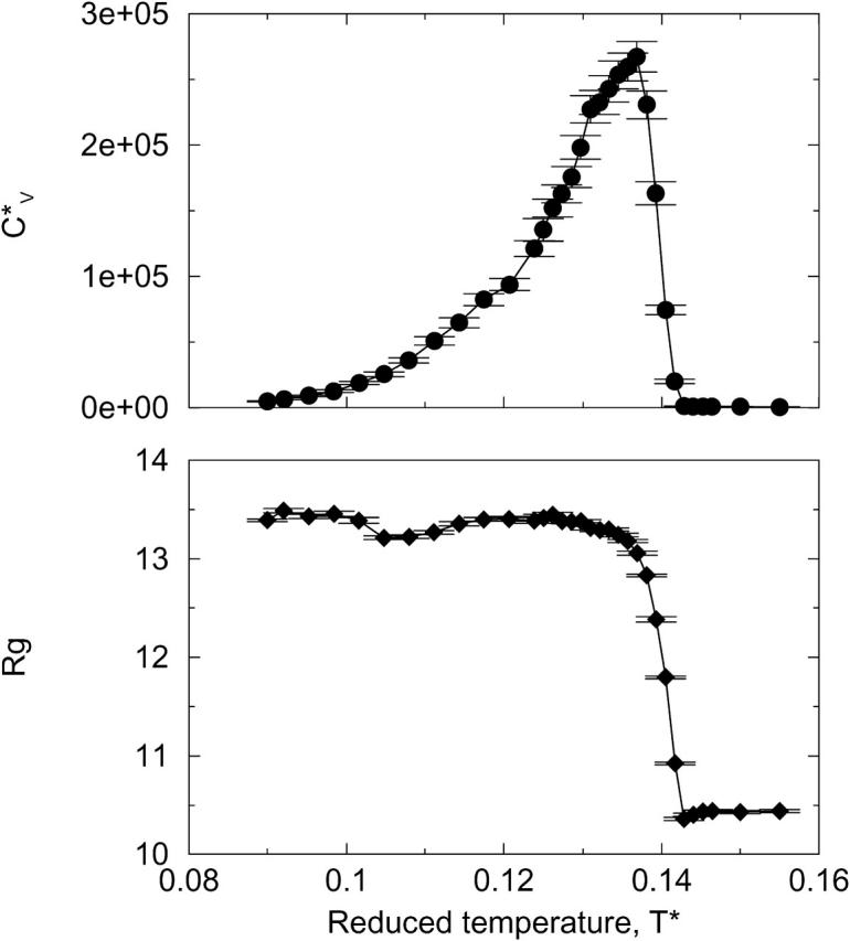
The thermodynamic properties  and Rg of the system at c = 3.5 mM show the same phase transition as that inferred from the data in Fig. 10. This can be seen in Fig. 11, which plots the reduced specific heat
  and radius of gyration Rg (in Å) as a function of the reduced temperature T* for the same system as in Fig. 10. The specific heat results show a peak at T* = 0.13, which corresponds to the upper limit of the temperature region in which the number of fibrils is at a maximum. The radius of gyration also indicates that there is a phase transition between fibrils and random coils as its value drops from 13.2 Å at T* = 0.12 to 11.0 Å at T* ≥ 0.14. In addition, the value of the radius of gyration is consistent with an increase in the percentage of peptides that form fibrils over the lower range of the transition temperature as its value increases from 12.0 Å at T* = 0.09 to 13.2 Å at T* = 0.13.
FIGURE 11.
Reduced specific heat  and radius of gyration Rg (in Å) versus the reduced temperature T* for the 96-peptide system at c = 3.5 mM.
As the concentration increases from c = 3.5 mM to c = 5.0 mM, there is again only a phase transition between fibrils and random coils. This can be seen in Fig. 12, which plots the percentage of peptides in different structures as a function of the reduced temperature T* for the 96-peptide system at c = 5.0 mM. Over a wide temperature range from T* = 0.09 to T* = 0.14, a high percentage (80%) of the peptides form fibrils and a low percentage (∼15%) form nonfibrillar β-sheets. At T* > 0.14, most peptides form random coils.
FIGURE 12.

The percentage of peptides in α-helices (•), fibrils (□), nonfibrillar β-sheets (♦), amorphous aggregates (▵), hairpins (▴), and random coils (*) versus the reduced temperature T* for the 96-peptide system at c = 5.0 mM.
The thermodynamic properties  and Rg of the system at c = 5.0 mM show the transition between fibrils and random coils. This can be seen in Fig. 13, which plots the reduced specific heat
  and radius of gyration Rg (in Å) as a function of the reduced temperature T* for the same system as in Fig. 12. The transition is at ∼T* = 0.135, which is slightly lower than the midpoint of the fibril transition at T* = 0.139 shown in Fig. 12.
FIGURE 13.
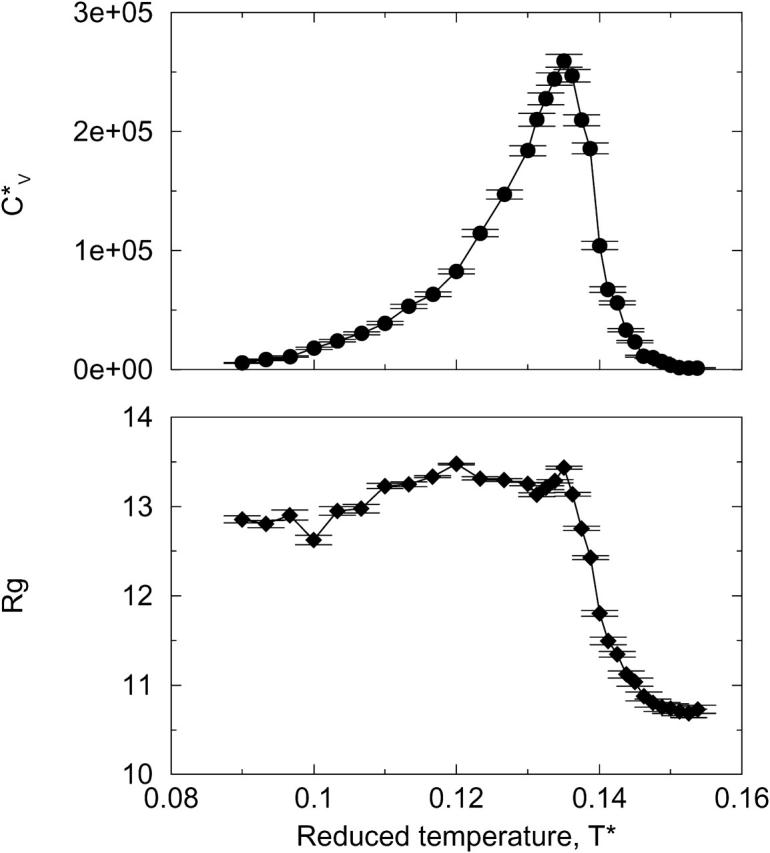
Reduced specific heat  and radius of gyration Rg (in Å) versus the reduced temperature T* for the 96-peptide system at c = 5.0 mM.
The results for the 96-peptide system that we have just described are summarized in Fig. 14, which shows the phases that occur in the space spanned by the reduced temperature T* and peptide concentration c. Here we call a particular structure a phase if the percentage of peptides forming that structure is at least 50%. If the structure with the second-highest percentage of peptides has a percentage of at least 20%, we then say that there are two phases. If no structure has a percentage of 50% or higher, we then say that there are two phases, which contains the two structures with the highest percentages. Fig. 14 shows that there are four single-phase regions: α-helices, fibrils, nonfibrillar β-sheets, and random coils. In addition, there are four different two-phase regions: random coils/nonfibrillar β-sheets, random coils/fibrils, fibrils/nonfibrillar β-sheets, and α-helices/nonfibrillar β-sheets. When one of the phases in a two-phase region is dominant, this is indicated by an all-caps label on Fig. 14.
FIGURE 14.

Phase diagram for the 96-peptide system as a function of the reduced temperature, T*, and peptide concentration, c. The single-structure phases are α-helices, fibrils, nonfibrillar β-sheets (shown as non-fib sheets), and random coils. The two-phase regions are random coils/nonfibrillar β-sheets, random coils/fibrils, fibrils/nonfibrillar β-sheets, and α-helices/nonfibrillar β-sheets.
The formation of the various structures of interest is highly dependent upon the peptide concentration and temperature:
At low concentrations (c ≤ 0.5 mM), there are two transitions separating the following three regions: a single-phase region containing α-helices at low temperatures (T* ≤ 0.11); a two-phase region containing random coils and nonfibrillar β-sheets at intermediate temperatures (T* = 0.12–0.13); and a single-phase region containing random coils at high temperatures (T* > 0.13).
As the concentration is increased to c = 1.0 mM, the number of α-helices formed at low temperatures (T* ≤ 0.10) decreases as nonfibrillar β-sheets are increasingly formed.
As the temperature is increased to intermediate temperatures (T* = 0.11–0.13) at c = 1.0 mM, the formation of nonfibrillar β-sheets increases. Further increase in the temperature results in the formation of random coils.
As the concentration is increased to c = 2.0 mM, there is a transition between a two-phase region (containing fibrils and nonfibrillar β-sheets) at low and intermediate temperatures (T* < 0.14); and a single-phase region containing random coils at high temperatures.
As the concentration is increased to c = 3.5 mM, there are two transitions between a two-phase region (containing fibrils and nonfibrillar β-sheets) at low temperatures; a one-phase region containing fibrils at intermediate temperatures; and a single-phase region containing random coils at high temperatures.
As the concentration is increased beyond c = 3.5 mM, there are three transitions between a two-phase region (containing fibrils and nonfibrillar β-sheets) at low temperatures; a one-phase region containing fibrils at intermediate temperatures; a two-phase region (containing fibrils and random coils) at high temperatures; and a single-phase region containing random coils at very high temperatures.
Note that the more the concentration is increased above 3.5 mM, the more the fibril region expands to low temperatures. Although Fig. 14 indicates that in the high concentration region (c > 2.5 mM) fibril formation is independent of the concentration at T* > 0.10, the degree of fibril formation actually increases with the concentration. This can be seen by comparing the percentages of peptides that are fibrils shown in Fig. 10 with those in Fig. 12.
The formation of the various structures of interest depends upon the outcome of the competition between intramolecular and intermolecular interactions. Intramolecular interactions predominate at low temperatures and low concentrations, contributing to the formation of α-helices. As the concentration is increased to intermediate values, intermolecular interactions predominate at low to intermediate temperatures, contributing to the formation of nonfibrillar β-sheets As the concentration is increased further to high concentrations, intermolecular interactions predominate strongly at low to intermediate temperatures, contributing to the formation of fibrils. At all concentrations and at high temperatures, both intramolecular and intermolecular interactions lose out to the high kinetic energy, contributing to the formation of random coils.
CONCLUSIONS
In this article, we performed equilibrium simulations on 96-peptide systems over a very wide range of temperatures and peptide concentrations by using the replica-exchange simulation method. Based on the thermodynamic properties  and Rg of the system at each concentration and the data on the percentage of peptides that form the various structures, we mapped out a phase diagram in the temperature-concentration plane delineating the regions where different structures are stable. We found that there are four distinctive single-phase regions: α-helices, fibrils, nonfibrillar β-sheets, and random coils. The α-helical region occurs at low temperature and low concentration. The β-sheet structures that are not in fibrils are at intermediate temperatures; this β-sheet region expands to higher temperatures as concentration is increased. The fibril region occurs mostly at intermediate temperatures and intermediate concentrations and expands to lower temperatures as the peptide concentration is increased. The random-coil region occurs at high temperatures at all concentrations and shifts to even higher temperatures as the concentration is increased. In addition, there are four different two-phase regions: random coils/nonfibrillar β-sheets, random coils/fibrils, fibrils/nonfibrillar β-sheets, and α-helices/nonfibrillar β-sheets.
It is important to point out that our model and analysis are subject to a number of limitations. First, we do not include charged residues at the ends of the model peptide chains, which have been shown to be important in experimental systems for reducing amorphous aggregation and precipitation. Second, it is possible that a more elaborate model force field is required to adequately represent peptides and their environment. Third, we have fixed the strengths of the hydrogen bond and hydrophobic interactions relative to temperature. Dill et al. (1989) and Shimuzu and Chan (2000) have proposed a temperature-dependent hydrophobic potential that undergoes a maximum at intermediate temperatures, accounting for weakened interactions from cold denaturation at low temperature and from heat denaturation at high temperature (Dill et al., 1989). Further simulation studies with our model will be required to probe the importance of temperature-dependent interactions. In addition, we have taken a majority rule approach in generating a phase diagram; therefore, each phase is not distinct in the sense that our two-phase regions do not represent equilibrium between two phases. Nevertheless, our phase diagram should prove useful in understanding the basic principles behind fibril formation since our results agree qualitatively with experiments on polyalanines by Blondelle and co-workers (Forood et al., 1995; Blondelle et al., 1997). They observed monomeric α-helical structures at 100 μM and 25°C. As the peptide concentration increased to 1 mM, they found that β-sheet complex formation increased with increasing temperature, exhibiting an S-shaped dependence on temperature with a critical temperature of 65°C. As the peptide concentration increased to 1.8 mM, they found that the critical temperature at which β-sheets start to form decreased to 45°C. It is hoped that our results, which are summarized in a phase diagram, will provide experimentalists some guidance in locating the temperature and concentration at which to conduct in vitro fibrillization experiments, or to avoid fibrillization. Although our phase diagram is not expected to be quantitatively accurate, especially for an arbitrary protein, we speculate that its shape may be universal. An experimentalist who is aware of this universal shape is less likely to conclude that fibrillization does not occur when the wrong region of the phase diagram is being accessed.
Although the model peptide studied, polyalanine, is perhaps not as exciting as other commonly studied amyloidogenic sequences such as those for β-amyloid, polyalanine was chosen for the study presented here because it is the simplest peptide known to form fibrils, and hence, the most easily modeled. The next step would be to add more features and parameters to our current model so as to accommodate all of the amino acids. Work along these lines is in progress but it is, of course, not a trivial undertaking. We believe that the modeling approach described in this article contributes to our molecular-level understanding of the fibrillization process, providing useful insights that could guide medical researchers in developing therapeutic strategies or inhibitors to treat the so-called amyloid diseases.
Acknowledgments
The authors are grateful to Sylvie Blondelle, Ken Dill, Jeffery Kelly, and Dan Kirschner for helpful discussions.
This work was supported by a grant from the National Institutes of Health (GM-56766) and a grant from the National Science Foundation (CTS-9704044).
References
- Alder, B. J., and T. E. Wainwright. 1959. Studies in molecular dynamics. I. General method. J. Chem. Phys. 31:459–466. [Google Scholar]
- Andersen, H. C. 1980. Molecular dynamics simulations at constant temperature and/or pressure. J. Chem. Phys. 72:2384–2393. [Google Scholar]
- Bellemans, A., J. Orban, and D. VanBelle. 1980. Molecular dynamics of rigid and non-rigid necklaces of hard discs. Mol. Phys. 39:781–782. [Google Scholar]
- Blondelle, S. E., B. Forood, R. A. Houghten, and E. Perez-Paya. 1997. Polyalanine-based peptides as models for self-associated β-sheet complexes. Biochemistry. 36:8393–8400. [DOI] [PubMed] [Google Scholar]
- Brais, B., G. A. Rouleau, J. P. Bouchard, M. Farde, and F. M. S. Tome. 1999. Oculopharyngeal muscular dystrophy. Semin. Neurol. 19:59–66. [DOI] [PubMed] [Google Scholar]
- Dill, K. A., D. O. V. Alonzo, and K. Hutchinson. 1989. Thermal stabilities of globular proteins. Biochemistry. 28:5439–5449. [DOI] [PubMed] [Google Scholar]
- Dima, R. I., and D. Thirumalai. 2002. Exploring protein aggregation and self-propagation using lattice models: phase diagram and kinetics. Prot. Sci. 11:1036–1049. [DOI] [PMC free article] [PubMed] [Google Scholar]
- Ding, F., N. V. Dokholyan, S. V. Buldyrev, H. E. Stanley, and E. I. Shakhnovich. 2002. Molecular dynamics simulations of the SH3 domain aggregation suggests a generic amyloidogenesis mechanism. J. Mol. Biol. 324:851–857. [DOI] [PubMed] [Google Scholar]
- Ding, F., J. M. Borreguero, S. V. Buldyrey, H. E. Stanley, and N. V. Dokholyan. 2003. Mechanism for the α-helix to β-hairpin transition. Proteins Struct. Funct. Genet. 53:220–228. [DOI] [PubMed] [Google Scholar]
- Dobson, C. M. 2001. The structural basis of protein folding and its links with human disease. Phil. Trans. R. Soc. Lond. B. 356:133–145. [DOI] [PMC free article] [PubMed] [Google Scholar]
- Esler, W. P., A. M. Felix, E. R. Stimson, M. J. Lachenmann, J. R. Ghilardi, Y. A. Lu, H. V. Vinters, P. W. Mantyh, J. P. Lee, and J. E. Maggio. 2000. Activation barriers to structural transition determine deposition rates of Alzheimer's disease Aβ amyloid. J. Struct. Biol. 130:174–183. [DOI] [PubMed] [Google Scholar]
- Fernandez, A., and M. D. L. Boland. 2002. Solvent environment conducive to protein aggregation. FEBS Lett. 529:298–302. [DOI] [PubMed] [Google Scholar]
- Fink, A. L. 1998. Protein aggregation: folding aggregates, inclusion bodies and amyloid. Fold. Des. 3:R9–23. [DOI] [PubMed] [Google Scholar]
- Forood, B., E. Perez-Paya, R. A. Houghten, and S. E. Blondelle. 1995. Formation of an extremely stable polyalanine β-sheet macromolecule. Biochem. Biophys. Res. Commun. 211:7–13. [DOI] [PubMed] [Google Scholar]
- George, A. R., and D. R. Howlett. 1999. Computationally derived structural models of the β-amyloid found in Alzheimer's disease plaques and the interaction with possible aggregation inhibitors. Biopolymers. 50:733–741. [DOI] [PubMed] [Google Scholar]
- Gsponer, J., U. Haberthur, and A. Caflisch. 2003. The role of side-chain interactions in the early steps of aggregation: molecular dynamics simulations of an amyloid-forming peptide from the yeast prion Sup35. Proc. Natl. Acad. Sci. USA. 100:5154–5159. [DOI] [PMC free article] [PubMed] [Google Scholar]
- Guo, Z., and D. Thirumalai. 1996. Kinetics and thermodynamics of folding of a de novo designed four-helix bundle protein. J. Mol. Biol. 263:323–343. [DOI] [PubMed] [Google Scholar]
- Harrison, P. M., H. S. Chan, S. B. Prusiner, and F. E. Cohen. 1999. Thermodynamics of model prions and its implications for the problem of prion protein folding. J. Mol. Biol. 286:593–606. [DOI] [PubMed] [Google Scholar]
- Horwich, A. L., and J. S. Weissman. 1997. Deadly conformations—protein misfolding in prion disease. Cell. 89:499–510. [DOI] [PubMed] [Google Scholar]
- Hwang, W., D. M. Marini, R. D. Kamm, and S. Zhang. 2003. Supramolecular structure of helical ribbons self-assembled from a β-sheet peptide. J. Chem. Phys. 118:389–397. [Google Scholar]
- Ilangovan, U., and A. Ramamoorthy. 1998. Conformational studies of human islet amyloid peptide using molecular dynamics and simulated annealing methods. Biopolymers. 45:9–20. [DOI] [PubMed] [Google Scholar]
- Irback, A., F. Sjunnesson, and S. Wallin. 2000. Three-helix-bundle protein in a Ramachandran model. Proc. Natl. Acad. Sci. USA. 97:13614–13618. [DOI] [PMC free article] [PubMed] [Google Scholar]
- Jang, H., C. K. Hall, and Y. Zhou. 2004a. Assembly and kinetic folding pathways of a tetrameric β-sheet complex: molecular dynamics simulations on simplified off-lattice protein models. Biophys. J. 86:31–49. [DOI] [PMC free article] [PubMed] [Google Scholar]
- Jang, H., C. K. Hall, and Y. Zhou. 2004b. Thermodynamics and stability of a β-sheet complex: molecular dynamics simulations on simplified off-lattice protein models. Prot. Sci. 13:40–53. [DOI] [PMC free article] [PubMed] [Google Scholar]
- Kelly, J. W. 1998. The alternative conformations of amyloidogenic proteins and their multi-step assembly pathways. Curr. Opin. Struct. Biol. 8:101–106. [DOI] [PubMed] [Google Scholar]
- Kelly, J. W. 2002. Towards an understanding of amyloidogenesis. Nat. Struct. Biol. 9:323–325. [DOI] [PubMed] [Google Scholar]
- King, J. 1989. Deciphering the rules of protein folding. Chem. Eng. News. 34:32–54. [Google Scholar]
- Kirschner, D. A., C. Abraham, and D. J. Selkoe. 1986. X-ray diffraction from intraneuronal paired helical filaments and extraneuronal amyloid fibers in Alzheimer disease indicates cross-β conformation. Proc. Natl. Acad. Sci. USA. 83:503–507. [DOI] [PMC free article] [PubMed] [Google Scholar]
- Kortvelyesi, T., G. Kiss, R. F. Murphy, B. Penke, and S. Lovas. 2001. Effect of Ala-substitution, N- and C-terminal modification and the presence of counter ions on the structure of amyloid peptide fragment 25–35. J. Mol. Struct. 545:215–223. [Google Scholar]
- Kusumoto, Y., A. Lomakin, D. B. Teplow, and G. B. Benedek. 1998. Temperature dependence of amyloid β-protein fibrillization. Proc. Natl. Acad. Sci. USA. 95:12277–12282. [DOI] [PMC free article] [PubMed] [Google Scholar]
- Lakdawala, A. S., D. M. Morgan, D. C. Liotta, D. G. Lynn, and J. P. Snyder. 2002. Dynamics and fluidity of amyloid fibrils: a model of fibrous protein aggregates. J. Am. Chem. Soc. 124:15150–15151. [DOI] [PubMed] [Google Scholar]
- Li, L., T. A. Darden, L. Bartolotti, D. Kominos, and L. G. Pedersen. 1999. An atomic model for the pleated β-sheet structure of Aβ amyloid protofilaments. Biophys. J. 76:2871–2878. [DOI] [PMC free article] [PubMed] [Google Scholar]
- Ma, B., and R. Nussinov. 2002a. Molecular dynamics simulations of alanine rich β-sheet oligomers: insight into amyloid formation. Prot. Sci. 11:2335–2350. [DOI] [PMC free article] [PubMed] [Google Scholar]
- Ma, B., and R. Nussinov. 2002b. Stabilities and conformations of Alzheimer's β-amyloid peptide oligomers (Aβ16–22, Aβ16–35, and Aβ10–35): sequence effects. Proc. Natl. Acad. Sci. USA. 99:14126–14131. [DOI] [PMC free article] [PubMed] [Google Scholar]
- Mager, P. P. 1998a. Molecular simulation of the amyloid β-peptide Aβ(1–42) of Alzheimer's disease. Mol. Sim. 20:201–222. [Google Scholar]
- Mager, P. P. 1998b. Molecular simulation of the primary and secondary structures of the Aβ(1–42)-peptide of Alzheimer's disease. Med. Res. Rev. 18:403–430. [DOI] [PubMed] [Google Scholar]
- Mager, P. P., R. Reinhardt, and K. Fischer. 2001. Molecular simulation to aid in the understanding of the Aβ(1–42) peptide of Alzheimer's disease. Mol. Sim. 26:367–379. [Google Scholar]
- Massi, F., and J. E. Straub. 2001a. Probing the origins of increased activity of the E22Q Dutch mutant Alzheimer's β-amyloid peptide. Biophys. J. 81:697–709. [DOI] [PMC free article] [PubMed] [Google Scholar]
- Massi, F., and J. E. Straub. 2001b. Structural and dynamical analysis of the hydration of the Alzheimer's β-amyloid peptide. J. Comput. Chem. 24:143–153. [DOI] [PubMed] [Google Scholar]
- Massi, F., J. W. Peng, J. P. Lee, and J. E. Straub. 2001. Simulation study of the structure and dynamics of the Alzheimer's amyloid peptide congener in solution. Biophys. J. 81:31–44. [DOI] [PMC free article] [PubMed] [Google Scholar]
- Massi, F., D. Klimov, D. Thirumalai, and J. E. Straub. 2002. Charge states rather than propensity for β-structure determine enhanced fibrillogenesis in wild-type Alzheimer's β-amyloid peptide compared to E22Q Dutch mutant. Prot. Sci. 11:1639–1647. [DOI] [PMC free article] [PubMed] [Google Scholar]
- Moraitakis, G., and J. M. Goodfellow. 2003. Simulations of human lysozyme: probing the conformations triggering amyloidosis. Biophys. J. 84:2149–2158. [DOI] [PMC free article] [PubMed] [Google Scholar]
- Nguyen, H. D., A. J. Marchut, and C. K. Hall. 2004. Solvent effects on the conformational transition of a model polyalanine peptide. Prot. Sci. 13:2909–2924. [DOI] [PMC free article] [PubMed] [Google Scholar]
- Nguyen, H. D., and C. K. Hall. 2004. Molecular dynamics simulations of spontaneous fibril formation. Proc. Natl. Acad. Sci. USA. 101:16180–16185. [DOI] [PMC free article] [PubMed] [Google Scholar]
- Rapaport, D. C. 1978. Molecular dynamics simulation of polymer chains with excluded volume. J. Phys. A Math. Gen. 11:L213–L217. [Google Scholar]
- Rapaport, D. C. 1979. Molecular dynamics simulation of polymer chains in solution. J. Chem. Phys. 71:3299–3303. [Google Scholar]
- Rochet, J. C., and P. T. Lansbury, Jr. 2000. Amyloid fibrillogenesis: themes and variations. Curr. Opin. Struct. Biol. 10:60–68. [DOI] [PubMed] [Google Scholar]
- Shimizu, S., and H. S. Chan. 2000. Temperature dependence of hydrophobic interactions: a mean force perspective, effects of water density, and nonadditivity of thermodynamic signatures. J. Chem. Phys. 113:4683–4700. [Google Scholar]
- Simmons, L., P. May, K. Tomaselli, R. Rydel, K. Fuson, E. Brigham, S. Wright, I. Lieberburg, G. Becker, D. Brems, and W. Li. 1994. Secondary structure of amyloid β peptide correlates with neurotoxic activity in vitro. Mol. Pharma. 45:373–379. [PubMed] [Google Scholar]
- Smith, A. V., and C. K. Hall. 2001a. Alpha-helix formation: discontinuous molecular dynamics on an intermediate-resolution protein model. Proteins Struct. Funct. Genet. 44:344–360. [DOI] [PubMed] [Google Scholar]
- Smith, A. V., and C. K. Hall. 2001b. Assembly of a tetrameric α-helical bundle: computer simulations on an intermediate-resolution protein model. Proteins Struct. Funct. Genet. 44:376–391. [DOI] [PubMed] [Google Scholar]
- Smith, A. V., and C. K. Hall. 2001c. Protein refolding versus aggregation: computer simulations on an intermediate-resolution protein model. J. Mol. Biol. 312:187–202. [DOI] [PubMed] [Google Scholar]
- Smith, S. W., C. K. Hall, and B. D. Freeman. 1997. Molecular dynamics for polymeric fluids using discontinuous potentials. J. Comp. Phys. 134:16–30. [Google Scholar]
- Straub, J. E., J. Guevara, S. Huo, and J. P. Lee. 2002. Long time dynamic simulations: exploring the folding pathways of an Alzheimer's amyloid Aβ-peptide. Acc. Chem. Res. 35:473–481. [DOI] [PubMed] [Google Scholar]
- Sugita, Y., and Y. Okamoto. 1999. Replica-exchange molecular dynamics method for protein folding. Chem. Phys. Lett. 314:141–151. [Google Scholar]
- Sunde, M., and C. Blake. 1997. The structure of amyloid fibrils by electron microscopy and x-ray diffraction. Adv. Prot. Chem. 50:123–159. [DOI] [PubMed] [Google Scholar]
- Wetzel, R. 1994. Mutations and off-pathway aggregation of proteins. Trends Biotech. 12:193–198. [DOI] [PubMed] [Google Scholar]
- Yang, M., M. Lei, and S. Huo. 2003. Why is Leu55-Pro55 transthyretin variant the most amyloidogenic: insights from molecular dynamics simulations of transthyretin monomers. Prot. Sci. 12:1222–1231. [DOI] [PMC free article] [PubMed] [Google Scholar]
- Zanuy, D., and R. Nussinov. 2003. The sequence dependence of fiber organization. A comparative molecular dynamics study of the islet amyloid polypeptide segments 22–27 and 22–29. J. Mol. Biol. 329:565–584. [DOI] [PubMed] [Google Scholar]
- Zanuy, D., B. Ma, and R. Nussinov. 2003. Short peptide amyloid organization: stabilities and conformations of the islet amyloid peptide NFGAIL. Biophys. J. 84:1884–1894. [DOI] [PMC free article] [PubMed] [Google Scholar]
- Zerovnik, E. 2002. Amyloid-fibril formation. Proposed mechanisms and relevance to conformational disease. Eur. J. Biochem. 269:3362–3371. [DOI] [PubMed] [Google Scholar]
- Zhou, Y., M. Karplus, J. M. Wichert, and C. K. Hall. 1997. Equilibrium thermodynamics of homopolymers and clusters: molecular dynamics and Monte Carlo simulations of systems with square-well interactions. J. Chem. Phys. 107:10691–10708. [Google Scholar]