Escaping free-energy minima

Abstract

We introduce a powerful method for exploring the properties of the multidimensional free energy surfaces (FESs) of complex many-body systems by means of coarse-grained non-Markovian dynamics in the space defined by a few collective coordinates. A characteristic feature of these dynamics is the presence of a history-dependent potential term that, in time, fills the minima in the FES, allowing the efficient exploration and accurate determination of the FES as a function of the collective coordinates. We demonstrate the usefulness of this approach in the case of the dissociation of a NaCl molecule in water and in the study of the conformational changes of a dialanine in solution.

Molecular dynamics (MD) and the Monte Carlo simulation method have had a very deep influence on the most diverse fields, from materials science to biology and from astrophysics to pharmacology. Yet, despite their success, these simulation methods suffer from limitations that reduce the scope of their applications. A severe constraint is the limited time scale that present-day computer technology and sampling algorithms explore. In particular, there are many circumstances where the free energy surface (FES) has several local minima separated by large barriers. Examples of these situations include conformational changes in solution, protein folding, first-order phase transitions, and chemical reactions. In such circumstances a simulation started in one minimum will be able to move spontaneously to the next minimum only under very favorable circumstances. A host of methods have been suggested to lift this restriction and explore the FES (1–13) or to characterize the transition state (14, 15). Here we propose a solution to this problem by combining the ideas of coarse-grained dynamics (16, 17) on the FES (10, 12) with those of adaptive bias potential methods (2, 11), obtaining a procedure that allows the system to escape from local minima in the FES and, at the same time, permits a quantitative determination of the FES as a byproduct of the integrated process.

Methodology

We shall assume here that there exists a finite number of relevant collective coordinates s_i, i = 1,n where n is a small number, and we consider the dependence of the free energy ℱ(s) on these parameters. Practical examples of appropriate choices of these variables will be given below. The exploration of the FES is guided by the forces F = −∂ℱ/∂s. To estimate these forces efficiently, we introduce an ensemble of P replicas of the system, each obeying the constraint that the collective coordinates have a preassigned value s_i = s, and each evolved independently at the same temperature T. Since the P replicas are statistically independent, the estimate of thermodynamic observables (e.g., the forces on the constraints) is improved with respect to an evaluation on a single replica, and it can be parallelized in a straightforward manner. The constraints are imposed on each replica via the standard methods of constrained molecular dynamics (18) by adding to the Lagrangean a term Σ_i=1,nλ_i(s_i −s) where λ_i are Lagrange multipliers. Averaging over the time and over the replicas we can evaluate the derivative of the free energy relative to s as F = 〈λ_i〉 (1, 4). For the sake of simplicity we neglect here the small kinematic correction term discussed in ref. 4, although this can be added easily. Taking a cue from the work of Kevrikidis et al. (16), we use these forces, determined by microscopic dynamics, to define coarse-grained dynamics in the space of the s_is. In our case the definition of these dynamics is rather arbitrary and designed only to explore the FES efficiently. The dynamics is defined from the discretized evolution equation:

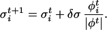In Eq. 1 we have introduced the scaled variables σ = s/Δs_i and the scaled forces φ = FΔs_i, where Δs_i is the estimated size of the FES well in the direction s_i, |φ^t| is the modulus of the n-th dimensional vector φ and δσ is a dimensionless stepping parameter. It should be stressed that Eq. 1 has the form of a steepest descent equation in the direction given by the forces φ_i and does not imply any real dynamical evolution. The index t is only used to label the states. After the collective coordinates are updated by using Eq. 1, a new ensemble of replicas of the system with values σ is prepared, and new forces F are calculated for the next iteration. At the same time the driving forces are evaluated from the microscopic Hamiltonian in short standard microscopic MD runs. Since there is no dynamical continuity between the P replicas at different iterations, one can use large values of δσ and move very efficiently in the space of the collective coordinates.

Clearly Eq. 1 alone cannot guarantee an efficient exploration of the FES, nor is it useful to determine the FES. This task can be achieved if we replace the forces in Eq. 1 with a history-dependent term (2, 11):

where the height and the width of the Gaussian W and δσ are chosen to provide a reasonable compromise between accuracy and efficiency in exploring the FES, as we will show below. The component of the forces coming from the Gaussian will discourage the system from revisiting the same spot and encourage an efficient exploration of the FES. As the system diffuses although the FES, the Gaussian potentials accumulate and fill the FES well, allowing the system to migrate from well to well. After a while the sum of the Gaussian terms will almost exactly compensate the underlying FES well. A typical example of this behavior is shown in Fig. 1, in which the dynamics in Eq. 1 is used to explore a one-dimensional potential energy surface (PES) V(σ) with three wells. The dynamics start from a local minimum that is filled by the Gaussians in ≈20 steps. Then the dynamics escapes from the well from the lowest energy saddle point, filling the second well in ≈80 steps. The second highest saddle point is reached in ≈160 steps, and the full PES is filled in a total of ≈320 steps. Hence, in the case of this example, since the form of the potential is known, it can be verified that, for large t and if the width of the Gaussians is sufficiently small with respect to the length of a typical variation of V,

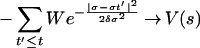modulus an additive constant. The same property can be verified for any multidimensional potential if the variables σ_i are allowed to vary in a finite region. Hence, we assume that Eq. 3 holds also if the method is used to explore the FES, and that the free energy can be estimated from Eq. 3 for large t. This procedure resembles the algorithm recently proposed by Wang and Landau (11), in which a time-dependent bias is introduced to modify the density of states to produce locally flat histograms.

Fig 1.

Time evolution of the sum of a one-dimensional model potential V(σ) and the accumulating Gaussian terms of Eq. 2. The dynamic evolution (thin lines) is labeled by the number of dynamical iterations (Eq. 1). The starting potential (thick line) has three minima and the dynamics is initiated in the second minimum.

We observe an interesting isomorphism between our dynamics and the ordered deposition of the beads of a polymer chain on the FES. In fact, we can regard σ as the position of a monomer in the n-dimensional parameter space. Each monomer is held at a distance δσ from the previous one and monomers repel each other with the Gaussian term of Eq. 2. Neglecting terms of order δσ² each monomer is placed by Eq. 1 in the position of free energy minimum compatible with the requirement of minimum overlap with previous beads. Hence, the polymer chain generated in this manner fills the wells in the FES. This isomorphism helps to clarify how our approach works and why it can be made more precise by reducing δσ.

The efficiency of the method in filling a well in the PES (or in the FES) can be estimated by the number of Gaussians that are needed to fill the well. This number is proportional to (1/δσ)ⁿ, where n is the dimensionality of the problem. Hence, the efficiency of the method scales exponentially with the number of dimensions involved. If n is large, the only way to obtain reasonable efficiencies is to use Gaussians with a size comparable to that of the well. On the other hand, a sum of Gaussians can only reproduce features of the FES on a scale larger than ≈δσ. A judicious choice of Δs_i, W, and δσ will ensure the right compromise between accuracy and sampling efficiency, and the optimal height and width of the Gaussians are determined by the typical variations of the FES.

If prior information on the nature of the free-energy well is not available, the scaling parameters Δs_i are chosen by performing short coarse-grained dynamic runs without bias potential (see Eq. 1). In such a case the system moves around the minimum. The scaling parameters are chosen so that the elongations have approximately the same value in all directions. This amounts to an empirical form of preconditioning that makes the FES minimum nearly spherical in n dimensions and easy to fill with n-dimensional Gaussians.

The metastep length δσ determines the efficiency of the method in a manner that is exponential in n and it should be made as large as possible. However, the dynamics in Eq. 1 is able to reconstruct details of the FES only on the length scale of δσ. Moreover, an over-large value of δσ would cause the system to jump irregularly from one basin to the other. The value of δσ is chosen requiring the metatrajectory to remain localized in the FES minimum if the bias potential is not applied. With this choice of δσ, a single step of the dynamics in Eq. 1 cannot lead a system from a FES minimum to another, and the initial state at each new iteration can be generated from the last MD step of the previous iteration without creating major overlaps. Since the shake algorithm is used to impose a new set of σ values, large forces on the constraints are generated at the beginning of each microscopic dynamics, and the initial part of the trajectory has to be discarded for the calculation of F.

The height of the Gaussians W can be estimated as follows. We notice that we want to reach a situation in which the modified FES is flat. In such a case the forces coming from the FES and that coming from the Gaussian approximately balance each other. If we require the maximum value of the Gaussian forces to be smaller than the typical FES force, we arrive at the relation W/δσe^−1/2 = α〈F〉^1/2 with α < 1. In all cases so far studied a value of α close to 0.5 allows a fast escape from the local minima in the FES without significant loss of the underlying structure.

In the future adaptive ways of determining all of these parameters should be considered for adapting the procedure in an optimal manner to the local shape of the FES.

Results

Dissociation of NaCl in Water.

We first discuss an application of the method to the dissociation of a NaCl molecule in water. The most stable state is the dissociated one, whereas the undissociated contact ion pair corresponds to a metastable local minimum. Here we shall study how the system escapes from this metastable state. We model the system by using the AMBER95 force field (20) and solvate the NaCl complex in 215 TIP3P water molecules with periodic boundary conditions. The electrostatic interaction between classical atoms is taken into account by the P3M method (19). As collective coordinates, we use the distance r_Na-Cl between Na and Cl, and, to take into account the dynamics of the solvation shell during the dissociation, we also use the electric fields V_Na and V_Cl on the Na and on the Cl due to the water molecules within ≈6.5 Å of the ions. V_Na and V_Cl depend significantly on the hydration pattern around the Na and on the Cl ion. If, for example, a hydrogen bond to one of the two ions is formed or broken, the field on the ion changes by several kcal/mol. A dynamic of the form in Eq. 1 was performed on the system, with δσ = 0.25 and W = 0.3 kcal/mol. The scaling parameters Δs_i were 0.53 Å, 32 and 32 kcal/mol for r_Na-Cl, V_Na, and V_Cl, respectively. The forces in Eq. 1 were evaluated by short MD runs with a time step of 0.7 fs performed on six replicas of the system. The replicas were equilibrated for 200 MD steps at 300 K, and the forces were evaluated by averaging over the following 500 MD steps. Starting from a distance of 2.6 Å, corresponding to a contact pair, the ions dissociate after 120 coarse-grained iterations. The dynamics was then continued for another 350 steps, imposing a maximum separation of the ion pair of 5 Å, to study the structure of the FES around the transition state (see Fig. 2). Seven recrossings for the coarse-grained dynamics were observed. The transition state is located r_Na-Cl ≈4.02 Å, V_Na ≈−120 kcal/mol, and V_Cl ≈81.5 kcal/mol (see Fig. 2). The overall topology of the FES confirms the importance of the solvent degrees of freedom for describing the reaction, since the transition region is in transverse orientation relative to the axis of the coordinates (21), and hence neither the distance nor the fields alone can provide an exhaustive description of the dissociation. The transition barrier (S in Fig. 2), estimated with thermodynamic integration (4) along r_Na-Cl, is of 3.3 kcal/mol. The one-dimensional free energy as a function of r_Na-Cl can also be obtained by integrating the three-dimensional FES (F₃) with respect to V_Na and V_Cl as F₁ = 1/βlog[∫dV_NadV_Cl exp(−βF₃)]. This leads to a barrier of 3.4 kcal/mol. Hence, the method is able to reproduce the one-dimensional free energy profile estimated with thermodynamic integration.

Fig 2.

Free energy as a function of the collective coordinates r_Na-Cl, V_Na, and V_Cl for a Na-Cl complex in water. The two-dimensional free energy F₂ shown here are obtained as F₂ = −1βlog[∫dz exp(−βF₃)], where β is the inverse temperatures, z is the coordinate not shown here, and the three-dimensional free energy F₃ is estimated with Eq. 3. The contours are plotted every 0.5 kcal/mol. The zero of the free energy corresponds to the metastable minimum of F in the contact ion pair (C).

We have verified that these collective coordinates identify the transition state and the reaction coordinate also in the dynamical sense (14). To this effect we prepared a set of replicas of the system with the critical values of the collective coordinates. We then followed the procedure described in ref. 21, assigning to the particles values of the velocity chosen from a Maxwellian distribution at 300 K, and following the trajectory backward and forward in time. By this procedure, we found that, within a time scale of 200 fs, the overwhelming majority of the replicas fell into one of the two basins of attraction without any recrossing. Moreover, the time-reversed dynamics leads systematically to the opposite basin of attraction (14). Finally, if we prepare the systems with the shake algorithm (18) for a given value of the collective coordinates, and if the particle velocities are not reassigned before letting the system evolve freely, the time needed to go in either of the attraction basins is of the order of a few ps, and several recrossings are observed. This is due to the fact that the shake algorithm imposes zero velocities in the direction of the constraint and it is only after thermalization, which takes place in a time scale of picoseconds, that the collective coordinates acquire sufficient velocity to evolve toward the FES minima. This is a strong confirmation that we have identified the correct transition state.

To characterize the solvent structure during the dissociation, we have computed the Na–water pair correlation function at the transition state S. The coordination number, obtained by integrating the pair correlation function up to a distance of 3 Å, is 5.28. This value is consistent with the picture depicted in ref. 21, in which the sodium at the transition state is shown to be typically only 5-fold coordinated.

Isomerization of Alanine Dipeptide in Water.

As a second application, we used our method to explore the FES of an alanine dipeptide as a function of the backbone dihedral angles Φ and Ψ (ref. 22 and references therein). The system is described by the all-atom AMBER95 force field (20) and solvated in 287 TIP3P water molecules. The parameters of the coarse-grained dynamics of Eq. 1 are δσ = 0.25 and W = 0.25 kcal/mol, while the scaling parameters Δs_i are 60° for both Φ and Ψ. The other settings are the same as for the simulation of the Na-Cl complex. The FES of alanine dipeptide in water has been studied in detail by other authors [refs. 22 (and references therein) and 23], who identified several minima. Our dynamics (1) is able to capture the overall features of the FES extremely quickly. Starting from a configuration close to the state C_7eq [refs. 22 (and references therein) and 23], the dynamics fills this attraction basin in approximately 45 steps. The minimum is localized at Φ ≈ −80° and Ψ ≈ 150°. The estimated free energy at the saddle point is 2 kcal/mol higher than the free energy in C_7eq. This compares to a value of 2.1 kcal/mol obtained in ref. 22 by thermodynamic integration. Our estimate is obtained with 45 steps of coarse-grained dynamics on six replicas, corresponding to a total of only ≈120 ps of microscopic dynamics. After another 150 steps, the dynamics fills the attraction basin of the state α_r, which corresponds to the equilibrium configuration of the system, and recrosses to C_7eq. Finally, the dynamics visits the Φ > 0 region of the configuration space after ≈300 steps. In Fig. 3 we plot the free energy as a function of Φ and Ψ after 40, 100, and 200 steps of coarse-grained dynamics. Also small details of the free energy landscape, like the location of the saddle points and the presence of secondary minima [e.g., the state C₅ (23)], can be detected graphically after a few steps of coarse-grained dynamics. The one-dimensional free energy profile as a function of Ψ obtained by analytic integration of the FES reproduces the profile obtained in ref. 22 within 0.2 kcal/mol for all of the values of Ψ. Concerning the choice of the collective coordinates for this system, it should be remarked that the dihedral angles Φ and Ψ do not provide a complete description of the dialanine isomerization reaction (ref. 22 and references therein), and the real reaction coordinate also should take into account the solvent degrees of freedom. Still, our results show that the method is able to reproduce the overall feature of the FES even if relevant degrees of freedom are not explicitly included in the collective coordinate space. This shows that the neglected degrees of freedom, although relevant for determining the reaction coordinate, are associated with relatively small barriers and are sampled efficiently during the microscopic dynamics for each value of Φ and Ψ, despite the relatively short runs. This is due to the use of the replicas and to the ability of the dynamics to retrace the same region of parameter space during the dynamics.

Fig 3.

Free energy as a function of the backbone dihedral angles Φ and Ψ for an alanine dipeptide in water after 40, 100, and 200 steps of coarse-grained dynamics (1). The zero of the free energy corresponds to the state α_r, located at Φ = −63 and Ψ = −30. The contours are plotted every 0.2 kcal/mol. The state C_7eq is located at Φ = −70 and Ψ = 165 and 1.3 kcal/mol. Finally, the transition state between α_r and C_7eq is located at Φ = −80 and Ψ = 35 and 3.3 kcal/mol. If the dynamics is continued, less favorable areas of the phase space are explored (e.g., the region with Φ > 0), but the free energy differences reported here are unchanged within the accuracy of the calculation.

Discussion

The method is based on the combination of the ideas of coarse-grained dynamics (16) in the space defined by a few collective coordinates and the introduction of a history-dependent bias (2, 11). Constructing dynamics on a FES that depends on a few collective coordinates, we simplify enormously the complexity of the problem, which depends exponentially on the number of degrees of freedom. The FES is much smoother than the underlying PES and it is topologically simpler, with a greatly reduced number of local minima. The history-dependent bias prevents the system from visiting regions it has already explored. This term is crucial for the efficiency of the method: for example, Langevin dynamics in the space of the collective coordinates would provide scant information on the underlying FES and it would be slower in locating global minima. This has been checked by performing a Langevin dynamics for the dissociation of a NaCl molecule in water, with the same collective variables introduced in Results and adding to Eq. 1 a Gaussian noise at a temperature T that is gradually reduced (24). The number of evaluations of the forces required to converge to the minimum of the FES (i.e., the dissociated state) is well above 1,000, if the temperature is decreased with a logarithic schedule, as required to ensure quasi-ergodicity in the collective coordinate space (25). A history-dependent bias potential as defined in Eq. 2 but applied in a regular MD simulation without coarse graining the dynamics would be efficient in finding escapes from the local minima, as has been shown (2), but it would not provide quantitative information about the FES. In particular, Eq. 3 holds only because the dynamic is performed in the collective coordinates space using the derivatives of the free energy. Hence, both the coarse-grained dynamics on the FES and the history-dependent bias are essential ingredients of the method, and only their combination allows an efficient and accurate determination of the FES.

Another advantage of our search algorithm is that it can be easily parallelized over the P replicas, thus optimally exploiting present-day computer architectures and, moreover, does not require a very accurate determination of the forces. In fact, in model calculations on an analytic PES, we have found that the algorithm is effective even for noise levels as large as 20–30% of the forces, since the height and the width of the Gaussians is such that the coarse-grained dynamics explores a region of space of the size of a Gaussian several times. and the system is only discouraged (and not prevented) from revisiting the same spot of configuration space. Hence, the errors in the forces tend to even out during the evolution. The dynamics (1) is “self-healing,” i.e., it is in principle capable to compensate the effect of completely wrongly located Gaussians or of a wrong additional bias potential. We can therefore use quite short runs and a small number of replicas to evaluate the forces. This is at variance with thermodynamic integration (18) and the blue moon ensemble method (1, 4), where a very precise determination of the forces is needed and where treating multidimensional reaction coordinates is a daunting task. Other techniques, like the umbrella sampling or bias potential methods (5, 6, 9, 18), allow an accurate estimate of the FES in many dimensions. The drawback of these methods is that they are efficient only if a good approximation for the FES is known a priori, whereas this is not required in our method.

A last advantage of the method is its ability to provide qualitative information on the free energy of a system in a very short time. For example, the overall topology of a FES can be determined by very few coarse-grained dynamics steps by using large Gaussians. Subsequently, our qualitative knowledge of the FES can be improved by using smaller Gaussians, eventually reducing the dimensionality of the problem by exploiting the topological information obtained with the large Gaussians.

Abbreviations

• FES, free energy surface

• PES, potential energy surface

• MD, molecular dynamics

References

- 1.Carter E. A., Ciccotti, G., Hynes, J. T. & Kapral, R. (1989) Chem. Phys. Lett. 156, 472-477. [Google Scholar]
- 2.Huber T., Torda, A. E. & van Gunsteren, W. F. (1994) J. Comput. 8, 695-708. [DOI] [PubMed] [Google Scholar]
- 3.Grubmüller H. (1995) Phys. Rev. E 52, 2893-2906. [DOI] [PubMed] [Google Scholar]
- 4.Sprik M. & Ciccotti, G. (1998) J. Chem. Phys. 109, 7737-7744. [Google Scholar]
- 5.Voter A. F. (1997) J. Chem. Phys. 106, 4665-4677. [Google Scholar]
- 6.Voter A. F. (1997) Phys. Rev. Lett. 78, 3908-3911. [Google Scholar]
- 7.Steiner M. M., Genilloud, P.-A. & Wilkins, J. W. (1998) Phys. Rev. B 57, 10236-10239. [Google Scholar]
- 8.Gong X. G. & Wilkins, J. W. (1999) Phys. Rev. B 59, 54-57. [Google Scholar]
- 9.VandeVondele J. & Rothlisberger, U. (2000) J. Chem. Phys. 113, 4863-4868. [Google Scholar]
- 10.Okuyama-Yoshida N., Kataoka, K., Nagaoka, M. & Yamabe, T. (2000) J. Chem. Phys. 113, 3519-3524. [Google Scholar]
- 11.Wang F. & Landau, D. P. (2001) Phys. Rev. Lett. 86, 2050-2053. [DOI] [PubMed] [Google Scholar]
- 12.VandeVondele J. & Rothlisberger, U. (2002) J. Phys. Chem. B 106, 203-208. [Google Scholar]
- 13.Rahman J. A. & Tully, J. C. (2002) J. Chem. Phys. 116, 8750-8760. [Google Scholar]
- 14.Bolhuis P. G., Chandler, D., Dellago, C. & Geissler, P. (2002) Annu. Rev. Phys. Chem. 59, 291-318. [DOI] [PubMed] [Google Scholar]
- 15.Passerone D. & Parrinello, M. (2001) Phys. Rev. Lett. 87, 108302-108305. [DOI] [PubMed] [Google Scholar]
- 16.Kevrekidis, I. G., Theodoropoulos, C. & Gear, C. W. (2002) Comput. Chem. Eng., in press.
- 17.Weinan, E. & Engquist, B. (2002) arXiv e-Print archive, http://arxiv.org/abs/physics/0205048.
- 18.Allen M. P. & Tieldslay, D. J., (1987) Computer Simulations of Liquids (Clarendon, Oxford).
- 19.Hünenberger P. (2001) J. Chem. Phys. 23, 10464-10476. [Google Scholar]
- 20.Cornell W. D., Cieplak, P., Bayly, C. I., Gould, I. R., Jr., Merz, K. M., Ferguson, D. M., Spellmeyer, D. C., Fox, T., Caldwell, J. W. & Kollman, P. A. (1995) J. Am. Chem. Soc. 117, 5179-5197. [Google Scholar]
- 21.Geissler P. L., Dellago, C. & Chandler, D. (1999) J. Phys. Chem. 103, 3706-3710. [Google Scholar]
- 22.Bolhuis P. G., Dellago, C. & Chandler, D. (2000) Proc. Natl. Acad. Sci. USA 97, 5877-5882. [DOI] [PMC free article] [PubMed] [Google Scholar]
- 23.Apostolakis J., Ferrara, P. & Caflish, A. (1999) J. Chem. Phys. 110, 2099-2108. [Google Scholar]
- 24.Kirkpatrick S., Gelatt, C. D., Jr. & Vecchi, M. P. (1983) Science 220, 671-680. [DOI] [PubMed] [Google Scholar]
- 25.Geman S. & Geman, D. (1984) IEEE Trans. Pattern Anal. Machine Intell. 6, 721-741. [DOI] [PubMed] [Google Scholar]