Diffusion in Two-Component Lipid Membranes—A Fluorescence Correlation Spectroscopy and Monte Carlo Simulation Study

Abstract

Using fluorescence correlation spectroscopy, calorimetry, and Monte Carlo simulations, we studied diffusion processes in two-component membranes close to the chain melting transition. The aim is to describe complex diffusion behavior in lipid systems in which gel and fluid domains coexist. Diffusion processes in gel membranes are significantly slower than in fluid membranes. Diffusion processes in mixed phase regions are therefore expected to be complex. Due to statistical fluctuations the gel-fluid domain patterns are not uniform in space and time. No models for such diffusion processes are available. In this article, which is both experimental and theoretical, we investigated the diffusion in DMPC-DSPC lipid mixtures as a function of temperature and composition. We then modeled the fluorescence correlation spectroscopy experiment using Monte Carlo simulations to analyze the diffusion process. It is shown that the simulations yield a very good description of the experimental diffusion processes, and that predicted autocorrelation profiles are superimposable with the experimental curves. We believe that this study adds to the discussion on the physical nature of rafts found in biomembranes.

INTRODUCTION

The recent finding of nano- and mesoscale domains in biological membranes has strongly increased the interest in the physical factors that determine membrane organization. For the past three decades, the common understanding of biological membranes was based on the Singer and Nicolson (1972) fluid mosaic model—which considered the lipid membrane to be a homogeneous fluid, containing proteins which are dissolved in the lipid matrix. Specific interactions between individual molecules are not considered. Thus, the Singer-Nicolson model implicitly assumes that no lateral heterogeneities within the membrane plane exist. However, when analyzing phase diagrams of lipid mixtures one has to conclude that phase separation is generally expected as a function of temperature and composition (e.g., Lee, 1977). This is even more to be expected in such complex multicomponent mixtures as the biological membrane. The mattress model by Mouritsen and Bloom (1984) proposed interactions dominated by the hydrophobic matching of neighboring membrane components. The possibility of protein aggregation and domain formation is a natural consequence of this concept. This view has been supported in various theoretical (Sperotto et al., 1989; Mouritsen and Jørgensen, 1995; Heimburg and Biltonen, 1996; Mouritsen, 1998) and experimental studies on model systems (Korlach et al., 1999; Bagatolli and Gratton, 1999, 2000b; Nielsen et al., 2000a,b; Feigenson and Buboltz, 2001; Ivanova et al., 2003). Since the finding of rafts (nanoscopic domains rich in cholesterol and sphingolipids) in biological membranes the interest has grown in domains as putative regulatory objects in signal transduction (Simons and Ikonen, 1997; Brown and London, 1998; Harder et al., 1998; Rietveld and Simons, 1998; Bagnat et al., 2000; Simons and Toomre, 2000; Edidin, 2003). This relates especially to the understanding of diffusion pathways. If one assumes a binary reaction between two proteins in membranes, which display different miscibilities in different domains, the reaction rate could well be controlled by the lateral organization of the membrane. This gives rise to a general physical control mechanism that does not require conformational changes of individual proteins. Processes of this kind are greatly under-investigated, although there are, meanwhile, a number of observations that favor this view. Synaptic fusion, for instance, is inhibited when cholesterol is removed from the presynaptic membrane and the formation of rafts is hindered (Lang et al., 2001). Thus, there is increasing evidence for the biological relevance of domain formation processes. Domain formation has long been theoretically predicted by Monte Carlo simulations, especially from Mouritsen's group in Denmark (e.g., Mouritsen and Jørgensen, 1995 and references therein), but also by other authors (Sugar et al., 1994; Heimburg and Biltonen, 1996). Such models are mostly based on lattice calculations with 2–10 different lipid states. An important parameter in such simulations, as mentioned, is nearest-neighbor interaction, which is partially driven by the hydrophobic effect. These interactions affect the cooperativity of transitions as well as domain sizes and shapes.

This article is dedicated to investigating diffusion processes in membranes containing domains. There are various methods that have been successful in investigating diffusion processes in organized membranes: Fluorescence recovery after photobleaching, i.e., FRAP (Vaz et al., 1989, 1990; Vaz and Almeida, 1991; Almeida et al., 1992a; Almeida and Vaz, 1995), fluorescence correlation spectroscopy, i.e., FCS (Eigen and Rigler, 1994; Korlach et al., 1999; Schwille et al., 1999a,b; Pramanik et al., 2000; Feigenson and Buboltz, 2001; Böckmann et al., 2003), and single particle tracking (Schmidt et al., 1995, 1996; Schütz et al., 1997; Sonnleitner et al., 1999; Harms et al., 1999, 2001). These techniques have been used on model as well as biological membranes. Other methods are nuclear magnetic resonance (Fisher, 1978; Kuo and Wade, 1999; Oradd et al., 2002), as well as neutron scattering (Tabony and Perly, 1990; König et al., 1992, 1995). Each of these methods has typical advantages and disadvantages, in particular in respect to their inherent timescales. When studying diffusion in lipid membranes, confocal microscopy techniques (FRAP, FCS) are sensitive on the millisecond-to-second timescale, which is the time regime that fluorescence labels within the membranes need to diffuse through a focus with a diameter of ∼500 nm. A typical value of the diffusion constant of fluid lipids is D = 4 × 10⁻⁸ cm² per s. Neutron scattering, on the other extreme, is sensitive on the picosecond timescale, which is the time regime of the scattering process (D = 1 × 10⁻⁷ − 4 × 10⁻⁶ cm² per s for fluid phase lipids). The translation by one lipid diameter is too slow to be monitored by neutron scattering (Böckmann et al., 2003). Dynamic information from this method therefore is believed to reflect confined motion within a potential defined by neighboring lipids (Vaz and Almeida, 1991).

There are also a number of models for diffusion in lipid membranes. In single component membranes it has been modeled using hydrodynamics theory by Saffman and Delbrück (1975) or free volume models (Galla et al., 1979). Various models for diffusion of membrane components have been explored by M. Saxton (for reviews, see Saxton and Jacobson, 1997 and Saxton, 1999). They are based on various assumptions concerning the geometry of obstacles (Saxton, 1987, 1990, 1994). This includes the possibility of lipid bilayers with coexisting gel and fluid domains (Saxton, 1993a). These studies are very helpful to get a feeling for the influence of complex objects on diffusion in two dimensions. In complex environments anomalous diffusion is often observed, meaning that the mean-square displacement deviates from (actually, anomalous diffusion is defined as ; Saxton and Jacobson, 1997), with the diffusion constant D. However, none of these models makes use of thermodynamics information of the system (although the experimental FRAP studies of Almeida and Vaz aim at this point). For lipid systems it is known that the domain formation is temperature- and concentration-dependent (Sugar et al., 1999, 2001). The diffusion constant in the fluid lipid phase is in the range of 4 × 10⁻⁸ cm² per s (Blume, 1993; Korlach et al., 1999), whereas it is much slower in the gel phase 10⁻¹⁶–10⁻⁹ cm² per s (in the latter case the values vary significantly in the literature). This may be partially due to diffusion along line defects in the ripple phase (Schneider et al., 1983). One could consider gel domains as obstacles in a fluid environment. The diffusion timescales are dependent on whether the gel domains are percolating. In this case, fluorescence recovery in a FRAP experiment may not be complete. On the other hand, the size and shape of the domains is time-dependent and therefore the obstacle dimensions are subject to fluctuations (van Osdol et al., 1989, 1991; Grabitz et al., 2002). For this reason the typical timescale of the fluctuations is likely to influence the diffusion behavior. Even in systems with percolating obstacles, fluctuations should eventually lead to complete fluorescence recovery. No model for such diffusion problems is (to our knowledge) available. Only Polson et al. (2001) applied a Monte Carlo model on cholesterol-containing membranes, which was based purely on first principles and thermodynamic knowledge, on the phase diagram that aimed in the direction of the study presented here.

In this article we investigate diffusion processes in binary lipid mixtures (DMPC/DSPC) using fluorescence correlation spectroscopy (FCS) on supported multilayers, and Monte Carlo simulations based on calorimetric information as well as on the typical time-constants from FCS. Lipid mixtures of DMPC and DSPC have been shown to display mesoscopic and macroscopic phase separations, both by confocal microscopy and by simulation (Sugar et al., 1999, 2001; Bagatolli and Gratton, 2000a). We use the model by Sugar et al. (1999) as a basis for the simulation of the diffusion process. The aim is to understand the lipid motion on the basis of a dynamic model that makes full use of the thermodynamic information of the system.

MATERIALS AND METHODS

Lipids were purchased from Avanti Polar Lipids (Birmingham, Al), fluorescence labels from Molecular Probes (Leiden, The Netherlands). Oriented multilamellar membranes of DMPC/DSPC mixtures were created by drying the lipid on a quartz coverslip from a dichloromethane/methanol solution in a high vacuum desiccator. The dry samples were then hydrated with distilled water and equilibrated for at least 1 h. Distilled water was used to avoid possible fluorescent impurities introduced by buffer molecules. The pH of the sample on the coverslip was determined to be between 5 and 6, far away from the pK values of phosphatidylcholine headgroups (below 2 and above 10 for phosphate and choline group, respectively). Subsequently the diffusion processes in the membranes were investigated by fluorescence correlation spectroscopy (FCS). In our inverted microscope setup we used a linearly polarized continuous wave 532-nm Nd:Yag laser (Laser 2000, Wessling, Germany) with a power of 5 mW. We used a 1.20 NA 60× water immersion objective (UPLAPO; Olympus) and a confocal setup with pinhole sizes of 30–100 μm. The magnification in the focal plane is 50×. The probe was mounted on optical table equipment with a piezoelectric nanopositioning XYZ-system. The fluorescence signal was detected by two SPCM-AQR-13 avalanche photo diodes (Laser Components, Olching, Germany) recording perpendicular polarizations. The perpendicular polarization was introduced for polarization measurements unrelated to this article. The correlation curves shown in this article are usually cross-correlation curves between these two channels. They were found to be identical to the autocorrelation curves of both channels in the time regime of interest, but to avoid certain short time artifacts related to the dead time of the photodiodes. The dead time is in the range of 50 ns. Two photons which are closer than 50 ns may therefore not be correctly recorded. In cross correlation the second photon is recorded by another diode and deadtime artifacts are reduced. As fluorescence markers we used TRITC-DPPE (Fig. 1), and DiI-C18. We performed calorimetric studies on pure lipid melting in the presence of five different fluorescence markers (DiI-C16, DiI-C18, TRITC-DHPE, BODIPY-C16, and DiD-C18). For most autocorrelation experiments the DiI-C18 label was used since it displayed the smallest perturbation of lipid melting profiles out of those five labels. This indicates best miscibility in both gel and fluid lipid phase (data not shown). Timescales were calibrated with a Rhodamine 6G solution at 296 K with a known diffusion coefficient of D = 3 · 10⁻⁶ cm² per s at 22°C. The signal from the two APDs was analyzed using a FLEX5000/fast correlator card (Correlator.com, Bridgewater, NJ). The setup is schematically shown in Fig. 1. To avoid photobleaching in samples with slow label diffusion (e.g., gel membranes) we used optical filters to attenuate the excitation intensity by up to 1000-fold. This resulted in a relatively high noise in the autocorrelation profile at short times, when measuring membranes containing gel domains (highest attenuation). The Triplett formation was quenched by addition of oxygen into the aqueous buffer (Calvert and Pitts, 1966).

FIGURE 1.

(Left) Schematic drawing of the FCS setup and the simulations. The laser (green) is focused on planar membranes, which are predicted to contain domains. Fluorescence light from the focus (yellow) is projected on two avalanche photodiodes (APD) which monitor different polarizations. In the image plane a pinhole is located. (Center) Single molecule fluorescence intensity traces of rhodamine 6G in solution, TRITC in a fluid lipid membrane and TRITC in a gel lipid membrane. Note the different timescales. (Right) Autocorrelation of the fluorescence signals shown in the center panel. The diffusion timescale within the fluid membrane is much faster than in the gel membrane, but approximately two orders-of-magnitude slower than the free diffusion of a label in the bulk solvent. The solid lines represent fits according to Eq. 1.

Assuming a Gaussian cross section of the focus, the correlation function in a planar system is given by

(1)

where N is the mean number and τ_d is the dwell-time of the labeled lipids in the focus (Korlach et al., 1999). The term in brackets is used as normalized correlation function, G_norm(τ). All correlation curves shown in this article are normalized profiles. Fitting experimental autocorrelation profiles sensitively depends on the assumption of a Gaussian focus (Hess and Webb, 2002), describing the detection intensity as a function of the distance from the focus center. This detection probability is a convolution of excitation profiles and pinhole properties (Rigler et al., 1993). In our experiments the autocorrelation profiles of the pure lipid phases were well described by the autocorrelation function in Eq. 1, indicating that the focus profile was close to being Gaussian. This fact is used later in the simulation of the autocorrelation profiles. Temperature control was achieved via water cooling of the objective and the sample cell. During the experiment (2–5 min) the water cooling was switched off to avoid mechanical vibrations. The temperature was measured with an ultra-thin thermocouple directly on the coverslip.

Calorimetry was performed using a high sensitivity differential VP-calorimeter (MicroCal, Northampton, MA) with scan rates of 5°/h.

To prepare the lipid half-spheres (LHS) from DLPC-DPPC mixtures for confocal microscopy we used the electroformation method (Angelova et al., 1992). Two microliters of lipid stock solution were spread on the conducting side of a coverslip coated with an indium tin oxide (ITO) layer and evaporated under a stream of nitrogen. The coated coverslips were purchased from PGO (Iserlohn, Germany) and subsequently abraded from 1 mm to 0.175 mm in the optical workshop of the MPI (Göttingen, Germany). The ITO coverslip with the lipid layer was then placed in a desiccator overnight to evaporate remaining solvent. Afterwards the ITO coverslip was placed into a cell with a second conducting coverslip, separated from the first one by a spacer with a thickness of 1.5 mm. The space between the conducting coverslips was filled with distilled water. The whole cell was sealed with vacuum grease and then inserted into a temperature-controllable stage, which was kept at ∼60°C during formation of LHS. The two coverslips were connected to an AC generator (H-Tronic, Hirschau, Germany) that produced an AC field with an amplitude of 3 V and a frequency of 10 Hz in the capacitor, which was applied for 30 min. After this procedure, the LHS were ready for experiments in a confocal microscope (Leica, Heidelberg, Germany), and were directly observed in the cell in which they were produced. The labels used in confocal microscopy were DiI-C18 and BODIPY-C16. These label have preferences for gel and fluid phases of DLPC-DPPC mixtures, respectively.

Monte Carlo simulations were performed on various desktop computers and workstations using self-written routines in C. We used the pseudo random-number generator ran2 as recommended by Press et al. (1997), which has a periodicity of 2 · 10¹⁸. With each simulation we newly initialized the random number generator with the computer time.

THEORY

Monte Carlo simulations

Let us consider a two-component lipid membrane with the lipid chains being located on a triangular lattice. The two chains of a lipid are covalently linked and occupy two adjacent sites on the triangular lattice, thus allowing for three different orientations. Each lipid chain may exist in two states, either gel or fluid. The two states are different in internal energy and in entropy. The Hamiltonian of such a system is given by

(2)

where and are the numbers of gel and fluid lipid chains of lipid species A and B, and the and are the respective internal energies of the two states of species A or B. The are the numbers of interactions between a lipid of species i in state α with a lipid of species j in state β, and the are the corresponding interaction energies. It has previously been shown that, on this basis, the Gibbs free energy for a given microconfiguration can be written as (Sugar et al., 1999)

(3)

where ΔH_A and ΔH_B are the calorimetric melting enthalpies, and ΔS_A = ΔH_A/T_m,A and ΔS_B = ΔH_B/T_m,B are the respective melting entropies of the two individual lipids, with T_m,A and T_m,B being the melting temperatures of the two pure components. G₀ is the Gibbs free energy of an all gel matrix without any unlike nearest-neighbor interactions. For our simulation we do not have to know this parameter since we are only interested in free energy differences. The are the nearest-neighbor interaction parameters of a lipid chain of species i in state α with a lipid chain of species j in state β (being simple functions of the ; see Sugar et al., 1999). The cooperativity parameters and determines the transition half-width of the single lipid melting profiles (Ivanova and Heimburg, 2001). Thus, of the 10 parameters, six can readily be determined from calorimetric experiments of single lipid membranes of species A and B. The other four parameters, , , , and , determine the shape of the phase diagram (Sugar et al., 1999). The phase space was explored by Monte Carlo simulations as described previously (Sugar et al., 1999; Ivanova and Heimburg, 2001). For this it is necessary to generate a lipid configuration of a computer lattice. The lipid chains are allowed to change state using Glauber algorithms (Glauber, 1963) and to diffuse in the plane by nearest-neighbor exchange of lipids as described in Fig. 2. Here we assumed that each lipid diffusion step goes into a random direction, which is correct if typical correlation lengths are shorter than molecular dimensions (Einstein, 1906). This was found to be true in recent MD simulations (Böckmann et al., 2003). As shown in Fig. 2, different diffusion steps were allowed, which were given the same a priori probability. This assumption is not founded on solid theoretical grounds. We have no detailed experimental knowledge on the molecular nature of the diffusion steps. The whole simulation is based on a two-dimensional Ising model which is clearly not correct on molecular scales since it only contains two states of the lipid, which is of course unrealistic. The two-dimensional Ising model has its strength in the description of macroscopic fluctuations (Mouritsen et al., 1983), irrespective of molecular details. Therefore, we assume that for the questions asked in this article the detailed molecular choice of a diffusion step is not important as long as we look at length scales of microscopic focus size.

FIGURE 2.

(Left) State changes from gel to fluid of individual lipid chains in the Monte Carlo simulation. (Right) Possible nearest-neighbor exchange steps of lipids leading to diffusion. On the simulation matrix the lipid chains are located on a triangular lattice. All individual exchange steps were explored with the same frequency. The link between the two chains of a lipid is indicated by a bar.

Simulation of an FCS experiment

Monte Carlo simulation

In the following we want to mimic the FCS experiment by Monte Carlo simulations, making use of the typical time constants from the FCS measurements. The Monte Carlo simulation is performed such that changes in chain state (gel or fluid), or the exchange of the position of two lipids, is done by randomly picking a lipid chain or two adjacent lipids on the matrix. The Gibbs free energy of the lattice is calculated before and after the change of the lattice state (see Fig. 2), and the likelihood that the new state is accepted is calculated according to a Boltzmann factor containing the free energy difference between the two states (Sugar et al., 1994). For the calculation of the equilibrium properties it does not matter whether the state changes between two consecutive Monte Carlo steps are physically realistic or not. The decision of whether or not to accept a new state is exclusively made on the basis of the free energy difference between the two states. For example, one can exchange lipid positions which are not localized on neighboring lattice sites, even though this process is very unlikely in a real lipid membrane. For this reason, Monte Carlo simulations do not usually contain information on timescales.

In this article we investigate the phase behavior of mixtures of the lipids DMPC and DSPC. The parameters for this mixture were determined by Sugar et al. (1999) and slightly modified by us on the basis of fits of calculated heat capacity profiles to differential calorimetry profiles of multilamellar vesicles. The parameter set that provided the best global fit to the melting profiles (see Fig. 3, right) of various DMPC-DSPC mixtures is given in Table 1. Fig. 3 (right) also shows the nice agreement between experiment and simulation. For other mixing ratios it is equally good. We assume in the following that differences between multilamellar and unilamellar systems are reflected in the melting profiles and therefore also in the simulation parameters. Unilamellar vesicles display less cooperative melting and for this reason probably smaller domains. We furthermore assume that the possible differences in diffusion timescales are caused by changes in domain arrangement and not by direct interactions of individual lipids in different layers. The parameters of our MC simulations, as mentioned, were obtained for multilamellar vesicles, which reflect the experimental situation in the FCS experiment (see below).

FIGURE 3.

(Left) Phase-diagram, showing lower and upper limits of the calorimetric events. Regions of expected microscopic or macroscopic separation of gel and fluid regions are in shaded representation. (Right) Heat capacity profile of a DMPC:DSPC 50:50 mixture (solid line), and the corresponding Monte Carlo simulation (symbols).

TABLE 1.

Monte Carlo simulation parameters

Tm,A = 297.1 K
Tm,B = 327.9 K
ΔHA = 13,165 J/mol
ΔHB = 25,370 J/mol
ΔSA = 44.31 J/mol per K
ΔSB = 77.36 J/mol per K

Parameters for the Monte Carlo simulation of DMPC-DSPC mixtures: DMPC = species A and DSPC = species B. The indices g and f correspond to the gel and fluid states, respectively. All numbers are given per lipid chain. These values are slightly modified as compared to Sugar et al. (1999).

From a tangent construction the lower and upper limits of the melting profile can be determined and plotted into a diagram. In Fig. 3 (left) it is shown how well the boundaries of the calorimetric experiment and the simulation coincide. This diagram is often called phase diagram in the literature (Lee, 1977). However, one should use this expression with great care. The existence of heat capacity anomalies does not necessarily mean that there is macroscopic phase separation. The definition of a phase as it was made by Gibbs requires macroscopic phase separation where the free energy of the domain interfaces can be neglected. This is clearly not the case for the mixtures in this article. Sugar et al. (2001) found that the regions of macroscopic demixing do not coincide with the outer limits of the heat capacity profile. In that article the distribution of domain sizes versus temperature has been quantified using the model also used here. In Fig. 3 the expected regions of local or global gel-fluid coexistence are shaded.

From the Monte Carlo simulation one can also deduce Monte Carlo snapshots, which are a graphical representation of a matrix configuration at a given time during the simulations. In Fig. 4 four snapshots at four different temperatures below, within and above the melting regime are shown. Red regions correspond to gel state lipids; green regions correspond to fluid chain lipids. The color code is the same as defined in Fig. 2. As can be readily seen, the snapshots at T = 302 K and T = 319 K contain, respectively, small fluid domains within a gel matrix, or small gel domains embedded into a fluid matrix. This situation does not reflect phase separation; instead, it reflects cooperative fluctuations in state. The other two snapshots at T = 305 K and T = 317 K do, however, reflect macroscopic phase separation, since at 305 K one macroscopic fluid domain of the same length scale as the matrix size exists, and at 315 K one macroscopic gel domain of the length scale of the matrix exists. Thus, one criteria for determining the existence of phase separation is whether or not domain sizes are on the order of the matrix size. For comparison, in Fig. 4 (right) the confocal microscopy image of four adjacent vesicles on an ITO coverslip are shown. These images were obtained from DLPC:DPPC = 30:70 mixtures at 306 K. The color code in the microscopic images is, for this purpose, the same as in the Monte Carlo simulations: red areas correspond to gel domains and green areas correspond to fluid domains. A striking similarity of the domain shapes between simulation and experiment can be seen, although one has to note that the snapshots shown correspond to ∼30 × 26 nm, whereas the diameters of the vesicles in Fig. 4 (right) are ∼15–25 μm. We here show a DLPC-DPPC mixture at room temperature because temperature control was difficult in the confocal microscopes available to us. However, the phase diagram of the DLPC-DPPC mixtures looks quite similar to the DMPC-DSPC diagram. The latter diagram is just shifted to higher temperatures. Therefore we assume a similar behavior. We also recorded a few low quality images of DMPC-DSPC vesicles at higher temperatures with a sample holder connected to a water bath (not shown). Domain formation was also found, although the domain shapes generally tended to be more elongated. In summarizing, however, the simulations seem to reflect the domain shapes found in experiments.

FIGURE 4.

(Left) Representative Monte Carlo snapshots of a 50:50 DMPC:DSPC mixture at four temperatures below, within, and above the melting regime (see Fig. 3).The color code is shown in Fig. 2. (Red domains correspond to gel lipids, green domains to fluid lipids.) Note the different length scales of the domains (macroscopic and microscopic domains). (Right) Confocal microscopy image of a 30:70 DLPC:DPPC mixture at 306 K, showing domain formation (gel domains in red, fluid domains in green). Compare with the domain shapes in the simulation.

Diffusion timescales

The apparent weakness that MC simulations do not contain timescales is also the strength of Monte Carlo simulations, because it allows us to calculate the thermodynamic properties of systems which fluctuate on very slow timescales. This is not possible with a method such as molecular dynamics. In this article, however, we want to calculate the timescales of lipid diffusion close to melting transitions. To this purpose one has to find means to include realistic timescales.

In principle it is possible to simulate time-dependent processes with Monte Carlo simulations if the individual Monte Carlo steps are chosen carefully. The temperature dependence of the relaxation behavior of single lipid membranes in the melting regime, for instance, was correctly predicted by autocorrelation of the enthalpy fluctuations during the MC simulation (Grabitz et al., 2002). However, to this purpose the Monte Carlo timescale has to be translated into a real timescale by a constant conversion factor that has to be taken from experiment. In fact, the basic concept in the famous Einstein articles on Brownian diffusion (Einstein, 1905, 1906) is to relate the fluctuation timescales to real timescales by comparison to the experiment (by introducing friction coefficients). In an MC simulation, the diffusion should be modeled by realistic translation steps as nearest-neighbor exchange, as compared to exchanging random lipids. As already mentioned, the latter case also yields all thermodynamics information but no realistic timescales.

In the present study we intend to simulate the diffusion behavior of lipids in the gel/fluid coexistence regime of a binary lipid mixture. It is known that the diffusion constant in the gel phase of lipids is several orders-of-magnitude smaller than the diffusion constant in the fluid phase. This is due to the fact that the gel membrane displays crystalline order of lipids within the membrane plane, whereas the fluid membrane is a random two-dimensional liquid. Also, the timescale of the enthalpy fluctuations is related to the heat capacity (Grabitz et al., 2002). Thus, there are three macroscopic timescales (state fluctuations, diffusion of lipids in a gel environment, and diffusion in a fluid environment), which have to be implemented into the Monte Carlo simulation. The conversion factors between simulation and experimental timescales may depend on the microenvironment of the lipids. This can be introduced into the simulation by making the decision to enter the different basic Monte Carlo processes (state changes, lipid exchange in gel, and fluid phase) with different frequencies. If the experimental diffusion timescale in the gel phase is two orders-of-magnitude smaller than in the fluid phase, the Monte Carlo routine that decides upon lipid translation is entered 100-fold less often. This mechanism still obeys detailed balance.

For lipids with an environment of both gel and fluid lipids, we made the probability of entering the translation routine of the program dependent on the fraction of gel lipid chains, f_c,g, surrounding the two lipids that are to be exchanged in a nearest-neighbor exchange process (including also the chains of the lipids). This procedure only affects the timescales but not the thermal equilibrium as long as all steps in the simulation obey detailed balance. We introduced a rate function r(f_c,g),

(4)

The rate r₀ is the probability to enter the lipid translation routine in the fluid phase (with f_c,g = 0). ΔE corresponds to the activation barrier for the exchange of two lipids in an all-gel environment (f_c,g = 1) and has to be calibrated by experiment. Practically, Eq. 4 defines a microviscosity by an activated process that depends on the lipid microenvironment. If two lipids are randomly chosen, the gel fraction in the environment of these lipids is determined, and the probability to enter the lipid exchange routine is adjusted according to the function r(f_c,g). This definition is necessary because lipids at the domain boundaries have both gel and fluid environments, and we therefore assume that they also display intermediate exchange rates. This approach has been chosen because experimental details of the physics of domain interfaces are not known. In a recent article (Ivanova et al., 2003) we have argued that the elastic constants at domain interfaces may be largely increased because gel-fluid fluctuations are maximum. Therefore the probability to obtain defects in the lipid matrix is possibly higher at domain interfaces. If diffusion occurs via a defect mechanism, diffusion along domain boundaries may be enhanced. Due to the lack of experimental data about these processes, however, we chose the simple definition of exchange rate constants described in Eq. 4. It may turn out in future studies that this approach is oversimplified.

In our experiments we found that diffusion in the gel phase was ∼70 times slower than in the fluid phase (Figs. 1 and 6). Consequently, we defined ΔE/kT ≈ 4.25, corresponding to the ratio of the exchange frequency in the fluid (f_c,g = 0) and in the gel phase (f_c,g = 1). The gel fraction on the circumference is determined for each pair of lipids. The probability to enter the translation routine is adjusted according to the factor r. To summarize: In the simulation we have three timescales. One is given by the frequency of trying a change in state of a lipid chain; the second defined by the frequency r₀ to try moving a lipid in the fluid phase; and the third is defined by the frequency r(f_c,g = 1) to move a lipid in the gel phase. The three frequencies are chosen by comparison with the experiment (see below). In most simulations shown here, the frequency r_state to attempt changes in lipid state has also been chosen to be equal to r₀. This is arbitrary, and the effect of changing this frequency is discussed below. In principle, this information is hidden in the FCS profile.

FIGURE 6.

Experimental and theoretical autocorrelation functions of three DMPC/DSPC mixtures at different temperatures. (Left) 70:30 mixture at 289.3 K, 303.0 K, 309.2 K, and 319.2 K (below, within, and above the melting regime; see Fig. 3). (Center) 50:50 mixture at 290.5 K, 303.6 K, 309.7 K, and 322.5 K (below, within, and above the melting regime). (Right) 30:70 mixture at 291.0 K, 317.6 K, and 330.0 K (below, within, and above the melting regime). The experimental profiles are very well described by the simulation. It shall be noted that the simulation exclusively relies on the calorimetric input parameters and does not require any fitting, except for the adjustment of the timescales in the pure gel and the pure fluid phases. All intermediate profiles are predictions rather than fits.

The FCS experiment in the simulation

In the FCS experiment, fluorescent dyes diffuse through a laser focus and produce a fluorescence signal on the photodiodes. It has been shown that the fluorescence detection profile of a confocal setup (being dependent on the excitation profile and the pinhole properties) is well approximated by a Gaussian cross section (Magde et al., 1972; Rigler et al., 1993). Since we perform FCS on a planar-supported membrane we do not have to worry about the focus profile in z direction. We can simulate the FCS experiment by randomly labeling some of the lipids in the simulation matrix with a virtual fluorescence marker, and we can record a simulated fluorescence intensity from each Monte Carlo snapshot (see Fig. 5). We assume that the fluorescence lifetime of the label is shorter than the nearest-neighbor exchange process. Assuming a diffusion constant in a fluid phase membrane of ∼4 × 10⁻⁸ cm² per s, the mean time period to move by one lipid diameter (7 Å) is ∼30 ns (see Böckmann et al., 2003), which is much longer than the mean life time of a fluorescence dye of ∼4 ns. Thus, in the simulation we assume instantaneous photon emission. The setup of the FCS simulation is shown in Fig. 5 (left). The concentric rings in this simulation indicate the Gaussian focus, the white dots mimic fluorescence markers which have randomly been placed on the lipids. During the simulation the markers move and generate a fluorescence intensity signal according to their position in the focus,

(5)

where r₀ is the coordinate of the focus center. This is exactly mimicking the situation in the experiment. A typical fluorescence intensity trace for a fluid membrane is shown in Fig. 5 (right upper panel). Fig. 5 (right bottom panel) shows the autocorrelation profile from the simulated fluctuating signal.

FIGURE 5.

(Left) The fluorescence correlation experiment can be simulated in the Monte Carlo simulation by labeling some of the lipid chains with a marker (white dots) and by introduction of a focus with Gaussian cross section (concentric circles). (Upper right panel) Assuming instantaneous emission after excitation with a Gaussian detection probability, a fluorescence signal from the diffusing labeled lipids can be obtained. (Lower right panel) Autocorrelated profile of the signal in the upper panel.

In more detail, we performed the FCS simulation such that, on a 60 × 60 lattice, 200 lipid chains were randomly labeled (open markers in Fig. 5, left). For this simulation the focus diameter was chosen to be 50 lipid chains. The dependence of the simulated fluorescence on focal radius is discussed below. The case that two chains within one lipid were labeled was prohibited. Hereby we assumed that DMPC and DSPC lipids were labeled with an equal probability. In the experiments, described below, we therefore used fluorescent markers with approximately equal partitioning in both lipid phases (as determined by calorimetry; see Materials and Methods).

The simulation itself made use of periodic boundary conditions. This means that a lipid that diffuses out of the left side of the simulation box returns to the box on the right-hand side. Now the problem may occur that the lipid diffusion may resemble that in a confined volume or corral (Saxton, 1993b) if the distance of a label from the focus center is not much larger than the focus diameter. Since the simulated focus size is of the same order as the lipid matrix, we tried avoiding boundary effects by keeping track of the distance of each label from the focus center by allowing for distances up to 2.5 simulation box diameters (corresponding to six times the focal radius). That means that even though a label may diffuse out of the simulation box on the left-hand side and reenter on the right side, we recorded the direction of the diffusion steps and calculated the effective distance from the focus center and calculated the detected fluorescence intensity accordingly. For autocorrelation, some authors considered virtual hardware correlators (Wohland et al., 2001) to correlate a simulated signal. Here, we instead saved the simulated fluorescence signal into a file and performed the autocorrelation after the simulation (G = F[F(I(t)) · F(I(t))*], with F and F* being Fourier transforms of the intensity trace). The simulated autocorrelation profiles of a pure gel or fluid lipid matrix display exactly the same shape as the experimental profiles. Furthermore, the simulated profile has the identical shape as a simple autocorrelation function described in Eq. 1. To check whether boundary effects are still present, we performed a control simulation where diffusion was followed over 13 times the simulated focus radius (actually over 330 lipid chain diameters). We found that the diffusion may have been slightly underestimated by using the smaller box size. However, this deviation is small (<10% of the diffusion constant) and is systematic (i.e., the same for all simulations). Therefore we assume that boundary effects are not significant in the interpretation of our data, and that our simulation correctly mimics the diffusion process.

Focus size

The observation volume in an experiment is in the range of 500 nm, depending on the pinhole size (between 30 and 100 μm). Taking a lipid chain diameter of ∼5 Å, this corresponds to ∼1000 × 1000 lipid chains. In this article we used smaller computer lattices in the range from 60 × 60 to ∼200 × 200 lipid chains. This corresponds to 30–100 nm. The main reason for this is limited computer time. Typically we performed Monte Carlo simulations with 2–20 · 10⁶ MC cycles. This is necessary to calculate the autocorrelation function over several orders of magnitude with reasonable accuracy. A calculation on a 60 × 60 matrix over this timescale takes ∼12 h on a 2-GHz desktop PC; and calculations on a 200 × 200 matrix uses computer times of approximately one week or longer, depending on the number of Monte Carlo steps. For this reason, under most circumstances, we worked with smaller matrix sizes. The effect of using simulation focus cross sections smaller than the experimental focus size is discussed below (see Results, below). However, it should be noted that the computer focus and the realistic experimental focus size are not too far apart.

RESULTS

The aim of the present study is to compare experimental FCS profiles with simulation to obtain insight into the domain structure and the timescales of binary lipid mixtures.

FCS experiments and comparison with the simulation

We performed FCS measurements on multilayered stacks of membranes at a given molar fraction of DSPC in DMPC. By using multilayered membranes we tried to minimize the possible effect of the interaction of the coverslip with the adjacent membrane. Since we know the concentration of fluorescence labels in the lipid membrane and also the focus size, we can deduce the number of lipid layers from the number of labels in the focus (see Eq. 1). In a typical experiment we had stacks of ∼50 bilayers. The whole microscope (sample cell and objective lens) was temperature-controlled by circulating water. Thus, the temperature could be adjusted with good accuracy. The absolute value of the temperature was obtained with a tiny thermocouple directly on the coverslip.

Fig. 6 shows the autocorrelation profiles of three different DMPC:DSPC mixtures at different temperatures. The curves with the fastest and slowest timescales in each panel correspond to pure fluid and gel phases, respectively. The timescales of these experiments were used to calibrate the diffusion timescales of the simulation defined by Eq. 4. The fluid and gel profiles in the three panels are nearly identical. Thus, the diffusion timescales in pure gel and fluid phases were roughly independent of the lipid mixing ratio. If we look at the phase-diagram in Fig. 3 one can predict that there are regions where gel and fluid state domains coexist. The intermediate profiles in the three panels reflect cases within this regime (see Fig. 3). However, it can clearly be seen that these profiles do not consist of a superposition of gel and fluid autocorrelation functions (see also Fig. 7, right, which is discussed below). The solid lines in Fig. 6 correspond to the Monte Carlo simulations, which are purely based on the thermodynamics information from the heat capacity profiles, using a unique set of simulation parameters (Table 1). The only numbers being changed in the simulation were temperature and composition. The theoretical profiles yield a surprisingly good description of the experimental profiles. It must be underlined again, that the theoretical profiles are predictions and are not fits. The information on the timescales originates from comparing the Monte Carlo timescale with the experimental timescales for the pure phases.

FIGURE 7.

(Left) The experimental autocorrelation profiles are subject to some variation due to changes in location within the sample and due to slight temperature variations. Here, for three different temperatures of a 70:30 DMPC:DSPC mixture, the mean variation of the autocorrelation profiles is shown. For Fig. 6 representative profiles were chosen, which are given here as solid lines. The dotted lines are the predictions from simulations shown in Fig. 6. (Right) This panel shows that the correlation profiles from the two-phase regime are not well described by a superposition of a pure gel (right curves) and a pure fluid component (left curves) with properties identical to the pure phase (the ratios of the two components have been chosen according to Fig. 3 using the Lever rule). The dotted lines are superpositions of analytical profiles according to Eq. 1. The profiles from the Monte Carlo simulations (which are identical to the experiment) are given by the solid lines. See text for a discussion.

Two things can be deduced from the quality of the computational prediction of the autocorrelation profiles:

1. The domain structures and the details of domain formation in the Monte Carlo description must be close to reality. Therefore it may be allowed to have a closer look at the simulation to learn about details of the domains and the phases (which are not the same).

2. The Monte Carlo simulation is well able to yield insight into the chain of events in the real membrane, and can therefore be used to analyze timescales.

First, however, some details of the measurement shall be discussed. The result of a diffusion experiment is subject to some scattering around a mean profile (Fig. 7). Most likely this scattering is due to different degrees of stacking in the multilayered sample, and may also depend on variations in the temperature of the confocal setup. Just as a side note, this scattering should also depend on the heat capacity of the samples, since the fluctuations in state depend on the heat capacity. Thus, in principle in an ideal experiment it might be possible to relate the fluctuations in autocorrelation to the heat capacity. We will explore this in more detail in future studies. In the present case, however, the uncertainties in the exact sample conditions are the likely cause of the variations in the autocorrelation profile. Fig. 7 (left) shows the variation at three different temperatures of a 70:30 DMPC:DSPC mixture. The profiles chosen for Fig. 6 are representative and not biased selections. Also shown in Fig. 7 (left) are the calculated profiles.

As discussed above, the autocorrelation profiles are not just superpositions of gel and fluid phase correlation functions (Fig. 7, right). If we construct an autocorrelation profile by superposition, we yield the form given in Eq. 6,

(6)

which clearly does not describe the experimental profile. It should, however, be noted that the autocorrelation can, in fact, be fitted by a two-component fit of the form given in Eq. 6, but with typical correlation times that deviate from τ_d,gel and τ_d,fluid (see also Korlach et al., 1999). The possible reason for this may be that embedded into a fluid phase region there are always some small domains of gel nature, and vice versa (see Fig. 4). Thus, it may not be surprising that the measured diffusion constants for the fast component within a mixed phase regime is slower than a pure fluid phase, and that the slow component is faster than a pure gel phase.

The simulations in Fig. 6, however, are predictions and no fits. The good agreement with the experimental data is a much more meaningful result than a fitted two-component profile, where the exact meaning of the two components is not clear (see Korlach et al., 1999).

The effect of focus size in the simulation

Most of the simulations shown in this article were performed on a 60 × 60 triangular lattice. Assuming a chain diameter of 5 Å, this box size corresponds to ∼30 nm × 25 nm. The focus diameter in these calculations was 50 chains corresponding to 25 nm. This is significantly smaller than the experimental focus diameter (depending on pinhole ∼500 nm ≅ 1000 chains). To investigate the influence of the simulation box size we performed some calculations on larger simulation matrices (80 × 80, and 200 × 200). As can be seen in Fig. 8 (left), increasing matrix size (and simultaneous increase in focus size) has only a minor influence on the autocorrelation profile. Small deviations seem, instead, to be a consequence of imperfect correlation due to limited length of the simulation. However, a 200 × 200 matrix size corresponds to 100 nm × 83 nm, which is nearly on the same order of magnitude as the experimental focus size. Our finding does not exclude that there are size effects on the autocorrelation profile. However, these differences are small in the range of the matrix and focus sizes investigated here.

FIGURE 8.

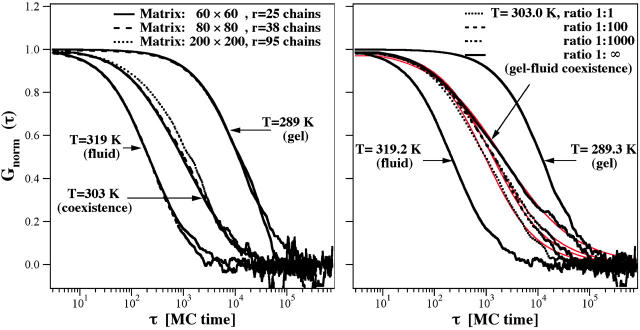
(Left) Dependence of the autocorrelation profile on increasing matrix and focal radius size: 60 × 60 with a focal radius of 25 chains, 80 × 80 with a focal radius of 38 chains, and 200 × 200 with a focal radius of 95 chains. The autocorrelation profiles are only slightly affected by the size of the simulation system. The 200 × 200 matrix corresponds to 100 nm × 83 nm, which is close to the experimental length scale. (Right) Dependence of the autocorrelation function on the relaxation timescale reflecting the frequency of attempts to change the state of a chain and to change position in the fluid state, indicated by a ratio of 1:1, 1:100, 1:1000, and 1:∞ (no state fluctuations). If the changes in state are less frequent than the positional changes, the slow components in the autocorrelation profile are more pronounced. This shows that the autocorrelation profile contains information about the relaxation timescales. The intermediate phase regime at all fluctuation rates could well be described by anomalous subdiffusion (red lines). Parameters are given in the text.

The effect of the relaxation timescale of lipid state fluctuations

Above, it was mentioned that the experimental autocorrelation profiles could also be described by two-component fits. The picture of having two different phases present may, however, be misleading. One can clearly see during the Monte Carlo simulation that over time gel domains may convert into fluid domains and vice versa. The timescale of these interconversions is closely related to the relaxation times of the fluctuations of state, which depend on the heat capacity (Grabitz et al., 2002). Relaxation times may be very long. For multilamellar vesicles they were found to be up to 45 s at the heat capacity maximum. For lipid mixtures one can therefore extrapolate that the relaxation time in the mixed phase regime is still on the order of 0.01–10 s. This is a comparable timescale to what a lipid in a gel or fluid environment needs to diffuse through the microscope focus. This means that during the time a lipid spends in the focus, its state (and therefore, its diffusion properties) may change. Thus, during the measurement of the autocorrelation profile (which takes 2–5 min) the properties of gel and fluid domains may, to a certain degree, be averaged out. We explored this possibility theoretically by changing the rate of flipping state (Glauber steps) as compared to the diffusion steps (Kawasaki steps) in the simulation (Fig. 8, right).

In the simulations shown in Fig. 6, we made the decision to enter the Monte Carlo routine making Glauber-steps with a similar frequency (r_state) than performing Kawasaki diffusion steps in the fluid phase (r(f_c,g = 0)). As described above, we used these frequencies to introduce timescales into the simulation. In reality the flipping and fluid diffusion timescales are likely to be different. The frequency of making the decision to flip a chain state, is closely related to the relaxation timescale of the state fluctuations of the lipid system (Grabitz et al., 2002). We explored different ratios of Glauber and Kawasaki step frequencies (Fig. 8, right). The ratios compared were r_state:r(f_c,g = 0) = 1:1, 1:100, 1:1000, and 1:∞ (lipid state changes switched off). The latter numbers mean that nearest-neighbor exchange in a fluid environment is increasingly faster than the change in chain state (in the last case state changes were completely switched off). Changes in the autocorrelation profile on altering r_state can be detected (Fig. 8, right). The amplitude of the autocorrelation curve on larger times increases when the state changes are performed less frequently.

This shows that, in principle, the autocorrelation profile contains information about the fluctuation timescales (similar to a relaxation experiment). In fact, some profiles in Fig. 6 might be slightly better described, if the slow time regime would be slightly more pronounced (see DMPC:DSPC = 70:30, 309.2 K, or DMPC:DSPC = 50:50, 303.6 K, respectively). However, these differences are small and probably within experimental error. Therefore, we conclude that the careful evaluation of the autocorrelation profiles also yields relaxation timescales of lipid state. However, in the present study we did not extract them due to the large standard deviation of experiments and simulations.

It may be interesting to notice that the autocorrelation profiles for the intermediate temperature regime in Fig. 8 (right) may well be fitted with an anomalous diffusion law , which in FCS assumes the form

(7)

where w is the focal radius (Schwille et al., 1999a) and D_a is the anomalous diffusion coefficient. The parameters in the fits of the profiles were

(8)

with τ in units of number of Monte Carlo cycles. This demonstrates that the apparent diffusion constant D_a in the fits to anomalous diffusion behavior changes, even though we only altered the fluctuation timescales in the simulation. The diffusion constants in gel and fluid state were the same in all those simulations. This also suggests that the physical insight obtained from fits to anomalous diffusion behavior may be rather limited if the microscopic origin of the parameters α and D_a is not known.

DISCUSSION

In this article we investigated the diffusion of lipids in planar membranes of two-component lipid mixtures. To this purpose we performed fluorescence correlation spectroscopy at various temperatures and mixing ratios of DMPC and DSPC. The autocorrelation profiles were compared with Monte Carlo simulations that made use of the thermodynamic properties of the DMPC-DSPC mixtures, which were obtained from calorimetry. Since Monte Carlo simulations do not contain timescales, they have to be introduced into the simulation by different frequencies to perform individual Monte Carlo steps. These frequencies were obtained by calibration with experimental data of the pure lipid phases from FCS. We arrived at a theoretical description that described the experimental autocorrelation data with a good accuracy. It should be noted that the simulations of the mixed phase regions were not attempts to fit the experimental data but, instead, were predictions based on thermodynamic information. We consider this to be an important step toward understanding diffusion processes in lipid membranes. Monte Carlo simulations yield information on the distribution of lipids, on the properties of phases and domains as well as on the thermal properties. The degree of accuracy, to which the predictions of the diffusion properties were possible, justifies the assumption that the Monte Carlo simulations provide an insight into the actual systems that is not far from reality. We showed that the autocorrelation profile not only contains information on diffusion timescales but also on relaxation timescales. Clearly, the autocorrelation profiles in mixed phase regions are not superpositions of a diffusion process in a pure fluid phase and another diffusion process in a pure gel phase (see Fig. 7, right). This is due to the fact that a lipid state can change while it travels through the microscope focus, and that domains may be smaller than the focal cross section. This also implies that the autocorrelation profiles on membranes, at least in principle, contain information on relaxation timescales, as we have shown in Fig. 8 (right)—although due to the accuracy of the data we were not able to resolve this information.

The present model makes use of lattice simulations performed by Monte Carlo methods. Monte Carlo simulations of lipid bilayer phase behavior, so far, have been nearly exclusively applied on monolayers (e.g., by Mouritsen, Pink, Sugar, and their collaborators). Not much is known about the coupling between the monolayers that form the bilayer. In a publication on the formation of the ripple phase we make use of monolayer coupling (Heimburg, 2000). Zhang et al. (1992) found that interbilayer coupling may increase cooperativity in the melting of the membrane. The fact that the heat capacity profiles of all mixtures can be described well by our simulation analysis on monolayers, to a certain degree justifies our assumption. Confocal microscopy imaging seems to indicate that some monolayer coupling is present since the domain distribution is usually identical in both monolayers. This effect, however, is likely to be already included in the choice of interaction parameters.

Diffusion of lipids in membranes has been measured by various methods, e.g., FRAP (Vaz and Almeida, 1991; Almeida et al., 1992a,b; Almeida and Vaz, 1995), and single particle tracking (Kusumi et al., 1993; Simson et al., 1995), which have partially been reviewed by Saxton and Jacobson (1997). In recent years, FCS has become more and more popular (Thompson, 1991; Korlach et al., 1999; Schwille et al., 1999a; Böckmann et al., 2003). FRAP and FCS measurements have the advantage over single particle tracking, in that one can sample easily over many events while having up to 100 particles in the focus. In single particle tracking, it can be quite difficult to obtain data with reasonable statistical significance (Qian et al., 1991). Other methods to measure diffusion are discussed in the Introduction.

Theoretically, there are various models by M. Saxton, partially reviewed in Saxton and Jacobson (1997) and Saxton (1999). Saxton distinguished mainly four kinds of diffusion processes:

1. Normal diffusion with 〈r²〉 = 4Dt.

2. Anomalous diffusion with 〈r²〉 = 4Dt^α (Saxton, 1994), (α < 1).

3. Diffusion with directed flow with 〈r²〉 = 4Dt + (Vt)².

4. Corralled motion, where molecules may diffuse freely within confined compartments within the membrane (Saxton, 1995).

In most of Saxton's models he considers immobile or mobile obstacles (Saxton, 1987, 1990) that hinder diffusion. The possible existence of percolating domains has, in particular, been highlighted by Almeida and Vaz (1995) by using FRAP. In their experiments they found that in lipid mixtures where gel and fluid phase coexist, the fluorescence recovery after photobleaching may be slow or incomplete. From this they concluded that domain structures exist which may be percolating. Under such conditions diffusion of fluorescence labels into a bleached area segment of the membrane is hindered or inhibited. Saxton modeled such processes in self-similar percolating clusters generated in a computer (Saxton, 2001). A recent model by Polson et al. (2001) calculated diffusion properties in cholesterol containing membranes on the basis of a 10-state model by Pink. This is, to our knowledge, the only previous work (except for the study presented here) that makes use of the thermodynamic information of the system under investigation. This study, however, lacks the direct comparison to the experiment that has been attempted in the present study. Therefore, we believe that the present study adds to our understanding of domain formation in lipid membranes. Our model assumes that diffusion takes place in both gel and fluid lipid domains. One result of the FCS measurements is that the diffusion constant in the gel membranes is ∼70 times smaller than in the fluid phase (D_fluid ≈ 4 × 10⁻⁸ cm² per s). The corresponding value of D ≈ 5 × 10⁻¹⁰ cm² per s is significantly higher than values reported by other methods. As mentioned in the Introduction, there is a considerable range of values reported for the gel phase, which depends on the time and length scale of the measurement. In our theoretical analysis we relied on the numbers we obtain from FCS. In FRAP, the diffusion constant in the gel phase was assumed to be much slower, and value down to D ≈ 10⁻¹⁶ cm² per s were reported. We cannot quite resolve the origin of this difference. Schneider et al. (1983) speculated that this may be due to line defect formation in the ripple phase. We have suggested that the ripple phase consists of periodic arrangements of fluid line defects (Heimburg, 2000). Many of our gel phase experiments may, in fact, be influenced by ripple formation. This may also explain the absence of polarization effects in our gel phase experiments. Korlach et al. (1999) found diffusion constants in DLPC-DPPC mixtures, which are in the range found by us (D_fluid = 3.9 × 10⁻⁸ cm² per s and D_gel = 2.1 × 10⁻¹⁰ cm² per s, respectively). Similar values were also reported in earlier literature for pure DPPC vesicles (Schneider and Webb, 1987). The diffusion processes measured by FCS were surprisingly well described by the Monte Carlo simulations.

Our simulations have several advantages over Saxton's models (which are usually of greater generality but less adjusted to a specific problem):

1. The thermodynamic parameters of the lipid mixture is correctly taken into account, meaning that our model makes correct predictions for all mixing ratios and temperatures.

2. The model allows for changes in relaxation times.

If we consider a gel domain as a soft obstacle (meaning that diffusion is slower but not forbidden in such domains), this obstacle may dissolve by fluctuations in lipid state during the measurement, or during the passage of a label through the microscopic focus. However, fluctuations in state are an intrinsic property of lipid membranes. The differences in the observed diffusion constant between FCS and FRAP may be a matter of observation volume and observation time. The choice of the fluorescence label may also play a role, since a label that does not partition in gel domains will consider them as obstacles, even if diffusion of other molecules in these domains is fast. We tried to rule out this possibility with the choice of our label. In the simulation, finite size effects in phase space regimes with macroscopic phase separation may also lead to the underestimation of long-range diffusion.

In this study, we are also able to perform single-particle tracking during the simulation (data not shown). One can obtain information on the mode of diffusion by plotting 〈r²〉/t as a function of time, which requires very long diffusion traces to reduce error bars (Qian et al., 1991), of typically >2,000,000 Monte Carlo steps, averaged over several dozen particles. The basic result of such an analysis is that in the melting regime of lipid mixtures there are basically three diffusion time regimes. For short processes diffusion is simple (case 1, above), because a label diffuses within one single domain. At intermediate timescales, diffusion is anomalous (case 2, above, displaying a fractal coefficient α < 1), because labels are sometimes in a gel and sometimes in a fluid environment and explore the heterogeneity of the system, when domain shapes and sizes may be complex. At long timescales diffusion is simple again (case 1, above), because the fluctuations of the lipid matrix average the heterogeneities on timescales larger than the relaxation time of the lipid matrix. Thus, it is obviously important whether obstacles have a lifetime or whether they are permanent. Our results on single particle trajectories will be described in detail in future publications.

We found from enthalpy correlation (Fig. 9) that typical timescales of domain size fluctuations are very dependent on temperature and composition, and may be slower or faster than the typical dwell-time of the label in the focus. In one of the curves shown (DMPC:DSPC 50:50 at 303.6 K, for a lipid-state change to lipid exchange, with a ratio of 1:1), one can observe dual relaxation times up to 3 × 10⁴ Monte Carlo cycles, corresponding to ∼1 s on an experimental scale (see comparison of Monte Carlo timescales to experimental timescales in Fig. 6). Since we concluded from the slight underestimation of the FCS autocorrelation profile in the mixed phase regime at longer times that the flipping ration may be larger (e.g., 1:1000 or more; see Fig. 8, right), relaxation timescales may be rather in the ⩾1000-s regime. In fluorescence and infrared quenching experiments by Jørgensen et al. (2000) it has been found for DC₁₆PC-DC₂₂PC mixtures that relaxations may take as long as 30 min or more. Although we could not adequately determine the relaxation time from our FCS experiment, these values are quite possible within the framework of our analysis. One should notice, however, that the whole experimental situation in Jørgensen et al. (2000) corresponded to a very large deviation from equilibrium accompanied by large compositional rearrangements, whereas our simulations are equilibrium simulations with only small fluctuations around an average value with small compositional rearrangements. Therefore their data may overestimate relaxation times in mixed lipid systems.

FIGURE 9.

Autocorrelation of the enthalpy fluctuations of a DMPC:DSPC mixture from the simulations in Fig. 6 (center panel), indicating the lipid state relaxation times (Grabitz et al., 2002). The typical steps in the enthalpy fluctuations yield the lipid state relaxation time(s). The relaxation at the c_P-maximum at 303.6 K is slowest, whereas it is fastest in the pure gel (290.5 K) and the fluid phases (322.5 K). Relaxation times at 303.6 K are between 10¹ and 10⁵ Monte Carlo cycles, whereas the mean dwell-time of the label is ∼10³ cycles. This indicates that relaxation processes may be slower than the time that a label spends in the microscope focus. For gel and fluid phase simulations (290.5 K and 322.5 K, respectively), relaxation is faster than the dwell-time of the label in the focus (see Fig. 6, center panel).

We take the good agreement between simulation and FCS experiment as an indication that the spatial picture created by the Monte Carlo snapshots is not far away from the truth. It may also help to interpret confocal microscopy images such as those shown in Fig. 4 (right panel). First of all, the snapshots in Fig. 4 show that the existence of domains is not identical to the macroscopic separation of phases. The snapshots at T = 305 K and T = 317 K show macroscopic separation of a phase of mainly fluid character (containing some small gel clusters) and a phase of mainly gel character (containing some fluid clusters). The snapshot at 302 K shows small fluid domains in a gel lipid matrix. The reverse case can be seen at 319 K, where small gel domains are found in a fluid matrix.

Thus, we find two different cases:

1. The separation into two phases, identical to separation into two macroscopic domains (containing small domains of the other state) of the length scale of the simulation box that grow with system size. Experimentally, domain sizes, to our knowledge, have never been studied systematically as a function of vesicle size. However, in some confocal microscopy studies, vesicles have been described that show macroscopic separation into just two domains with ordered and disordered chains (e.g., Baumgart et al., 2003).

2. Domains are smaller than the simulation system, and do not grow with system size. One can check this in the simulation by increasing the matrix size, or in an experiment on giant vesicles for vesicles of various size. Such an analysis is called finite-size scaling (Lee and Kosterlitz, 1991).

An example for such a case may serve from observations by Keller and McConnell (1999) regarding monolayers of binary lipid mixtures close to miscibility critical points. Small domains were seen with sizes depending on the distance from the critical point. In this article this was explained by competition between line tension at domain interfaces and electrostatic dipolar repulsion. In our notion this domain formation corresponds to critical fluctuations within the binary lipid matrix. For the system discussed here, finite-size scaling has been performed in Seeger et al., 2005).

When domains are not macroscopic, fluctuations per unit number of molecules are independent of system size (Ivanova and Heimburg, 2001), and the length of the overall domain interface is proportional to the size of the membrane (or the vesicle). We have shown for peptide-containing systems that the domain interfaces are the regions of large fluctuations (Ivanova et al., 2003). Since heat capacity, elastic constants, and relaxation timescales are a function of the fluctuations (Heimburg, 1998; Grabitz et al., 2002), the difference between a macroscopically phase-separated system and a microscopically fluctuating system (with no macroscopic phase separation) may be profound. This also implies that the existence of heat capacity anomalies does not automatically mean that there is a (first-order) transition, and that using the outer limits of a heat capacity profile to construct a phase diagram or analyzing domain areas in confocal microscopy (as was done, for example, by Feigenson and Buboltz, 2001) may be misleading not just because domains may exist within domains that are too small to be seen in the microscope. Sugar et al. (2001) have discussed this in more detail by analyzing domain size distributions as a function of temperature and composition in DMPC:DSPC mixtures. They found that the regime of phase separation does not coincide with the outer limits of heat capacity profiles. This also means that the finding of domains in a confocal microscopy image (Fig. 4) could indicate that there is a regime of phase separation. The interpretation is, of course, complicated by the fact that vesicles display a surface curvature, which influences the phase behavior and leads to domain rearrangement (Baumgart et al., 2003). In the ongoing discussion on the physical reality of rafts in biomembranes, it is of great importance to decide whether those nanoscopic domains represent phases (meaning that they are stable) or whether they are fluctuations (meaning that they are unstable domains that fluctuate in state, size, and time). The important difference arises from how sensitively such domains react to environmental changes, and whether such domain structures respond to controllable parameters in the cell (e.g., pH). The authors of this study favor such a view because it would make the rafts a controllable feature of the system, which should be in the interest of an organism. However, the possibility of rafts being stable units, on the basis of present experiments, cannot be ruled out. An article discussing aspects of finite-size scaling, and the relation between domain size and fluctuations at the domain boundaries, is in the submission process by Seeger et al., 2005.

Summarizing, we have presented here a diffusion study on membranes that directly relates thermodynamics information to diffusion experiments. In this combined FCS and Monte Carlo simulation study we demonstrated that diffusion processes in lipid mixtures can be well understood on the basis of extracting the thermodynamic properties of the lipid mixtures from calorimetry. Monte Carlo simulation presents the tool to determine the relevant parameters, leading to realistic predictions on domain formation and fluctuations in lipid state and position—which may, in the future, help understanding of the physical nature of domains in complex membranes.

References

- Almeida, P. F. F., and W. L. C. Vaz. 1995. Lateral diffusion in membranes. In Structure and Dynamics of Membranes: From Cells to Vesicles. R. Lipowski and E. Sackmann, editors. Elsevier, Amsterdam, The Netherlands. 305–357.
- Almeida, P. F. F., W. L. C. Vaz, and T. E. Thompson. 1992a. Lateral diffusion and percolation in two-phase, two-component lipid bilayers. Topology of the solid-phase domains in-plane and across the lipid bilayer. Biochemistry. 31:7198–7210. [DOI] [PubMed] [Google Scholar]
- Almeida, P. F. F., W. L. C. Vaz, and T. E. Thompson. 1992b. Lateral diffusion in the liquid phases of dimyristoylphosphatidylcholine/cholesterol lipid bilayers: a free volume analysis. Biochemistry. 31:6739–6747. [DOI] [PubMed] [Google Scholar]
- Angelova, M. I., S. Soleau, P. Meleard, J. F. Faucon, and P. Bothorel. 1992. Preparation of giant vesicles by external AC electric fields. Progr. Colloid Polym. Sci. 89:127–131. [Google Scholar]
- Bagatolli, L. A., and E. Gratton. 1999. Two-photon fluorescence microscopy observation of shape changes at the phase transition in phospholipid giant unilamellar vesicles. Biophys. J. 77:2090–2101. [DOI] [PMC free article] [PubMed] [Google Scholar]
- Bagatolli, L. A., and E. Gratton. 2000a. A correlation between lipid domain shape and binary phospholipid mixture composition in free-standing bilayers: a two-photon fluorescence microscopy. Biophys. J. 79:434–447. [DOI] [PMC free article] [PubMed] [Google Scholar]
- Bagatolli, L. A., and E. Gratton. 2000b. Two-photon fluorescence microscopy of coexisting lipid domains in giant unilamellar vesicles of binary phospholipid mixtures. Biophys. J. 78:290–305. [DOI] [PMC free article] [PubMed] [Google Scholar]
- Bagnat, M., S. Keranen, A. Shevchenko, and K. Simons. 2000. Lipid rafts function in biosynthetic delivery of proteins to the cell surface in yeast. Proc. Natl. Acad. Sci. USA. 97:3254–3259. [DOI] [PMC free article] [PubMed] [Google Scholar]
- Baumgart, T., S. T. Hess, and W. W. Webb. 2003. Imaging coexisting fluid domains in biomembrane models coupling curvature and line tension. Nature. 425:821–824. [DOI] [PubMed] [Google Scholar]
- Blume, A. 1993. Dynamic properties. In Phospholipids Handbook. G. Cevc, editor. Marcel Dekker, New York. 455–509.
- Böckmann, R. A., A. Hac, T. Heimburg, and H. Grubmüller. 2003. Effect of sodium chloride on a lipid bilayer. Biophys. J. 858:1647–1655. [DOI] [PMC free article] [PubMed] [Google Scholar]
- Brown, D. A., and E. London. 1998. Functions of lipid rafts in biological membranes. Annu. Rev. Cell Dev. Biol. 14:111–136. [DOI] [PubMed] [Google Scholar]
- Calvert, J. G., and J. N. J. Pitts. 1966. Photochemistry. Wiley, New York.
- Edidin, M. 2003. The state of lipid rafts: from model membranes to cells. Annu. Rev. Biophys. Biomol. Struct. 32:257–283. [DOI] [PubMed] [Google Scholar]
- Eigen, M., and R. Rigler. 1994. Sorting single molecules: application to diagnostic and evolutionary biotechnology. Proc. Natl. Acad. Sci. USA. 91:5740–5747. [DOI] [PMC free article] [PubMed] [Google Scholar]
- Einstein, A. 1905. Über die von der molekularkinetischen Theorie der Wärme geforderte Bewegung von in ruhenden Flüssigkeiten suspendierten Teilchen. Annals Phys. 17:549–560. [On the movement of small particles suspended in stationary liquids required by the molecular-kinetic theory of heat.] [Google Scholar]
- Einstein, A. 1906. Zur Theorie der Brownschen Bewegung. Annals Phys. 19:371–381. [On the theory of Brownian motion.] [Google Scholar]
- Feigenson, G. W., and J. T. Buboltz. 2001. Ternary phase diagram of dipalmitoyl-PC/dilauroyl-PC/cholesterol: nanoscopic domain formation driven by cholesterol. Biophys. J. 80:2775–2788. [DOI] [PMC free article] [PubMed] [Google Scholar]
- Fisher, R. W. 1978. Lateral diffusion of the phospholipid molecule in dipalmitoylphosphatidylcholine bilayers. An investigation using nuclear spin-lattice relaxation in the rotating frame. Biochemistry. 17:1177–1183. [DOI] [PubMed] [Google Scholar]
- Galla, H. J., W. Hartmann, U. Theilen, and E. Sackmann. 1979. On two-dimensional passive random walk in lipid bilayers and fluid pathways in biomembranes. J. Membr. Biol. 48:215–236. [DOI] [PubMed] [Google Scholar]
- Glauber, R. J. 1963. Time-dependent statistics of the Ising model. J. Math. Phys. 2:294–307. [Google Scholar]
- Grabitz, P., V. P. Ivanova, and T. Heimburg. 2002. Relaxation kinetics of lipid membranes and its relation to the heat capacity. Biophys. J. 82:299–309. [DOI] [PMC free article] [PubMed] [Google Scholar]
- Harder, T., P. Scheiffele, P. Verkade, and K. Simons. 1998. Lipid domain structure of the plasma membrane revealed by patching of membrane components. J. Cell Biol. 141:929–942. [DOI] [PMC free article] [PubMed] [Google Scholar]
- Harms, G. S., L. Cognet, P. H. M. Lommerse, G. A. Blab, H. Kahr, R. Gamsjager, H. P. Spaink, N. M. Soldatov, C. Romanin, and T. Schmidt. 2001. Single-molecule imaging of L-type Ca2+ channels in live cells. Biophys. J. 81:2639–2646. [DOI] [PMC free article] [PubMed] [Google Scholar]
- Harms, G. S., M. Sonnleitner, G. J. Schütz, H. J. Gruber, and T. Schmidt. 1999. Single-molecule anisotropy imaging. Biophys. J. 77:2864–2870. [DOI] [PMC free article] [PubMed] [Google Scholar]
- Heimburg, T. 1998. Mechanical aspects of membrane thermodynamics. Estimation of the mechanical properties of lipid membranes close to the chain melting transition from calorimetry. Biochim. Biophys. Acta. 1415:147–162. [DOI] [PubMed] [Google Scholar]
- Heimburg, T. 2000. A model for the lipid pretransition: coupling of ripple formation with the chain-melting transition. Biophys. J. 78:1154–1165. [DOI] [PMC free article] [PubMed] [Google Scholar]
- Heimburg, T., and R. L. Biltonen. 1996. A Monte Carlo simulation study of protein-induced heat capacity changes. Biophys. J. 70:84–96. [DOI] [PMC free article] [PubMed] [Google Scholar]
- Hess, S. T., and W. W. Webb. 2002. Focal volume optics and experimental artifacts in confocal fluorescence correlation spectroscopy. Biophys. J. 83:2300–2317. [DOI] [PMC free article] [PubMed] [Google Scholar]
- Ivanova, V. P., and T. Heimburg. 2001. A histogram method to obtain heat capacities in lipid monolayers, curved bilayers and membranes containing peptides. Phys. Rev. E. 63:1914–1925. [DOI] [PubMed] [Google Scholar]
- Ivanova, V. P., I. M. Makarov, T. E. Schäffer, and T. Heimburg. 2003. Analyzing heat capacity profiles of peptide-containing membranes: cluster formation of gramicidin A. Biophys. J. 84:2427–2439. [DOI] [PMC free article] [PubMed] [Google Scholar]
- Jørgensen, K., A. Klinger, and R. L. Biltonen. 2000. Nonequilibrium lipid domain growth in the gel-fluid two-phase region of a DC16PC-DC22PC lipid mixture investigated by Monte Carlo computer simulation, FT-IR, and fluorescence spectroscopy. J. Phys. Chem. B. 104:11763–11773. [Google Scholar]
- Keller, S. L., and H. M. McConnell. 1999. Stripe phases in lipid monolayers near a miscibility critical point. Phys. Rev. Lett. 82:1602–1605. [Google Scholar]
- König, S., T. Bayerl, G. Coddens, D. Richter, and E. Sackmann. 1995. Hydration dependence of chain dynamics and local diffusion in l-α-dipalmitoylphosphtidylcholine multilayers studied by incoherent quasi-elastic neutron scattering. Biophys. J. 68:1871–1880. [DOI] [PMC free article] [PubMed] [Google Scholar]
- König, S., W. Pfeiffer, T. Bayerl, D. Richter, and E. Sackmann. 1992. Molecular dynamics of lipid bilayers studied by incoherent quasi-elastic neutron scattering. J. Phys. II (Fr). 2:1589–1615. [Google Scholar]
- Korlach, J. J., P. Schwille, W. W. Webb, and G. W. Feigenson. 1999. Characterization of lipid bilayer phases by confocal microscopy and fluorescence correlation spectroscopy. Proc. Natl. Acad. Sci. USA. 96:8461–8466. [DOI] [PMC free article] [PubMed] [Google Scholar]
- Kuo, A. L., and C. G. Wade. 1999. Lipid lateral diffusion by pulsed nuclear magnetic resonance. Biophys. J. 77:2300–2308. [DOI] [PubMed] [Google Scholar]
- Kusumi, A., Y. Sako, and M. Yamamoto. 1993. Confined lateral diffusion of membrane receptors as studied by single particle tracking (nanovivid microscopy). Effect of calcium-induced differentiation. Biophys. J. 65:2021–2040. [DOI] [PMC free article] [PubMed] [Google Scholar]
- Lang, T., D. Bruns, D. Wenzel, D. Riedel, P. Holroyd, C. Thiele, and R. Jahn. 2001. Snares are concentrated in cholesterol-dependent clusters that define docking and fusion sites for exocytosis. EMBO J. 20:2202–2213. [DOI] [PMC free article] [PubMed] [Google Scholar]
- Lee, A. G. 1977. Lipid phase transitions and phase diagrams. II. Mixtures involving lipids. Biochim. Biophys. Acta. 472:285–344. [DOI] [PubMed] [Google Scholar]
- Lee, J., and J. M. Kosterlitz. 1991. Finite-size scaling and Monte Carlo simulations of first-order phase transitions. Phys. Rev. B. 43:3265–3277. [DOI] [PubMed] [Google Scholar]
- Magde, D., E. Elson, and W. W. Webb. 1972. Thermodynamic fluctuations in a reacting system: measurement by fluorescence correlation spectroscopy. Phys. Rev. Lett. 29:705–708. [Google Scholar]
- Mouritsen, O. G. 1998. Self-assembly and organization of lipid-protein membranes. Curr. Opin. Colloid Interface Sci. 3:78–87. [Google Scholar]
- Mouritsen, O. G., and M. Bloom. 1984. Mattress model of lipid-protein interactions in membranes. Biophys. J. 46:141–153. [DOI] [PMC free article] [PubMed] [Google Scholar]
- Mouritsen, O. G., A. Boothroyd, R. Harris, N. Jan, T. Lookman, L. MacDonald, D. A. Pink, and M. J. Zuckermann. 1983. Computer simulation of the main gel-fluid phase transition of lipid bilayers. J. Chem. Phys. 79:2027–2041. [Google Scholar]
- Mouritsen, O. G., and K. Jørgensen. 1995. Micro-, nano- and meso-scale heterogeneity of lipid bilayers and its influence on macroscopic membrane properties. Mol. Membr. Biol. 12:15–20. [DOI] [PubMed] [Google Scholar]
- Nielsen, L. K., T. Bjørnholm, and O. G. Mouritsen. 2000a. Critical phenomena—fluctuations caught in the act. Nature. 404:352. [DOI] [PubMed] [Google Scholar]
- Nielsen, L. K., A. Vishnyakov, K. Jørgensen, T. Bjørnholm, and O. G. Mouritsen. 2000b. Nanometre-scale structure of fluid lipid membranes. J. Phys. Condens. Matter. 12:309–314. [Google Scholar]
- Oradd, G., G. Lindblom, and P. W. Westerman. 2002. Lateral diffusion of cholesterol and dimyristoylphosphatidylcholine in a lipid bilayer measured by pulsed field gradient NMR spectroscopy. Biophys. J. 83:2702–2704. [DOI] [PMC free article] [PubMed] [Google Scholar]
- Polson, J. M., I. Vattulainen, H. Zhu, and M. J. Zuckermann. 2001. Simulation study of lateral diffusion in lipid-sterol bilayer mixtures. Eur. Phys. J. E. 5:485–497. [Google Scholar]
- Pramanik, A., P. Thyberg, and R. Rigler. 2000. Molecular interactions of peptide with phospholipid vesicle membranes as studied by fluorescence correlation spectroscopy. Chem. Phys. Lett. 104:35–47. [DOI] [PubMed] [Google Scholar]
- Press, W. H., S. A. Teukolsky, W. T. Vetterling, and B. P. Flannery. 1997. Random numbers. In Numerical Recipes in C, 2nd Ed. Cambridge University Press, Cambridge, UK. 274–283.
- Qian, H., M. P. Sheetz, and E. L. Elson. 1991. Single particle tracking: analysis of diffusion and flow in two-dimensional systems. Biophys. J. 60:910–921. [DOI] [PMC free article] [PubMed] [Google Scholar]
- Rietveld, A., and K. Simons. 1998. The differential miscibility of lipids as the basis for the formation of functional membrane rafts. Biochim. Biophys. Acta. 1376:467–479. [DOI] [PubMed] [Google Scholar]
- Rigler, R., U. Mets, J. Widengren, and P. Kask. 1993. Fluorescence correlation spectroscopy with high count rate and low background: analysis of translational diffusion. Eur. Biophys. J. 22:169–175. [Google Scholar]
- Saffman, P. G., and M. Delbrück. 1975. Brownian motion in biological membranes. Proc. Natl. Acad. Sci. USA. 72:3111–3113. [DOI] [PMC free article] [PubMed] [Google Scholar]
- Saxton, M. J. 1987. Lateral diffusion in an archipelago. The effect of mobile obstacles. Biophys. J. 52:989–997. [DOI] [PMC free article] [PubMed] [Google Scholar]
- Saxton, M. J. 1990. Lateral diffusion in a mixture of mobile and immobile particles: a Monte Carlo study. Biophys. J. 58:1303–1306. [DOI] [PMC free article] [PubMed] [Google Scholar]
- Saxton, M. J. 1993a. Lateral diffusion in an archipelago: dependence on tracer size. Biophys. J. 64:1053–1062. [DOI] [PMC free article] [PubMed] [Google Scholar]
- Saxton, M. J. 1993b. Single particle tracking: effects of corrals. Biophys. J. 65:389–398. [DOI] [PMC free article] [PubMed] [Google Scholar]
- Saxton, M. J. 1994. Anomalous diffusion due to obstacles: a Monte Carlo study. Biophys. J. 66:394–401. [DOI] [PMC free article] [PubMed] [Google Scholar]
- Saxton, M. J. 1995. Single-particle tracking: effect of corrals. Biophys. J. 69:389–398. [DOI] [PMC free article] [PubMed] [Google Scholar]
- Saxton, M. J. 1999. Lateral diffusion of lipids and proteins. Curr. Top. Membr. 48:229–282. [Google Scholar]
- Saxton, M. J. 2001. Anomalous subdiffusion in fluorescence photobleaching recovery: a Monte Carlo study. Biophys. J. 81:2226–2240. [DOI] [PMC free article] [PubMed] [Google Scholar]
- Saxton, M. J., and K. Jacobson. 1997. Single particle tracking: applications to membrane dynamics. Annu. Rev. Biophys. Biomol. Struct. 26:373–399. [DOI] [PubMed] [Google Scholar]
- Schmidt, T., G. J. Schütz, W. Baumgärtner, H. J. Gruber, and H. Schindler. 1995. Characterization of photophysics and mobility of single molecules in a fluid lipid membrane. J. Phys. Chem. 99:17662–17668. [Google Scholar]
- Schmidt, T., G. J. Schütz, W. Baumgärtner, H. J. Gruber, and H. Schindler. 1996. Imaging of single molecule diffusion. Proc. Natl. Acad. Sci. USA. 93:2926–2929. [DOI] [PMC free article] [PubMed] [Google Scholar]
- Schneider, M. B., W. K. Chan, and W. W. Webb. 1983. Fast diffusion along defects and corrugations in phospholipid P′β liquid crystals. Biophys. J. 43:157–165. [DOI] [PMC free article] [PubMed] [Google Scholar]
- Schneider, M. B., and W. W. Webb. 1987. Lipid membrane dynamics: biological cells, vesicles and smectic liquid crystals. In Physics of Complex and Supramolecular Fluids. S.A. Safran and N.A. Clark, editors. 179–208. Wiley.
- Schütz, G. J., H. Schindler, and T. Schmidt. 1997. Single-molecule microscopy an model membranes reveals anomalous diffusion. Biophys. J. 73:1073–1080. [DOI] [PMC free article] [PubMed] [Google Scholar]
- Schwille, P., U. Haupts, S. Maiti, and W. W. Webb. 1999a. Molecular dynamics in living cells observed by fluorescence correlation spectroscopy with one- and two-photon excitation. Biophys. J. 77:2251–2265. [DOI] [PMC free article] [PubMed] [Google Scholar]
- Schwille, P., J. Korlach, and W. W. Webb. 1999b. Fluorescence correlation spectroscopy with single molecule sensitivity on cell and model membranes. Cytometry. 36:176–182. [DOI] [PubMed] [Google Scholar]
- Seeger, H., M. Fidorra, and T. Heimburg. 2005. Domain size and fluctuations at domain interfaces in lipid mixtures. Macromolecular Symposia. In press.
- Simons, K., and E. Ikonen. 1997. Functional rafts in cell membranes. Nature. 387:569–572. [DOI] [PubMed] [Google Scholar]
- Simons, K., and D. Toomre. 2000. Lipid rafts and signal transduction. Nat. Rev. Mol. Cell Biol. 1:31–39. [DOI] [PubMed] [Google Scholar]
- Simson, R., E. D. Scheets, and K. Jacobson. 1995. Detection of temporary lateral confinement of membrane proteins using single-particle tracking analysis. Biophys. J. 69:989–993. [DOI] [PMC free article] [PubMed] [Google Scholar]
- Singer, S. J., and G. L. Nicolson. 1972. The fluid mosaic model. Science. 175:720–731. [DOI] [PubMed] [Google Scholar]
- Sonnleitner, A., G. J. Schütz, and T. Schmidt. 1999. Free Brownian motion of individual lipid molecules in biomembranes. Biophys. J. 77:2638–2642. [DOI] [PMC free article] [PubMed] [Google Scholar]
- Sperotto, M. M., J. H. Ipsen, and O. G. Mouritsen. 1989. Theory of protein-induced lateral phase separation in lipid membranes. Cell Biophys. 14:79–95. [DOI] [PubMed] [Google Scholar]
- Sugar, I. P., R. L. Biltonen, and N. Mitchard. 1994. Monte Carlo simulations of membranes: phase transition of small unilamellar dipalmitoylphosphatidylcholine vesicles. Methods Enzymol. 240:569–593. [DOI] [PubMed] [Google Scholar]
- Sugar, I. P., E. Michanova-Alexova, and P. Chong. 2001. Geometrical properties of gel and fluid clusters in DMPC/DSPC bilayers: Monte Carlo simulation approach using a two-state model. Biophys. J. 81:2425–2441. [DOI] [PMC free article] [PubMed] [Google Scholar]
- Sugar, I. P., T. E. Thompson, and R. L. Biltonen. 1999. Monte Carlo simulation of two-component bilayers: DMPC/DSPC mixtures. Biophys. J. 76:2099–2110. [DOI] [PMC free article] [PubMed] [Google Scholar]
- Tabony, J., and B. Perly. 1990. Quasielastic neutron scattering measurements of fast local translational diffusion of lipid molecules in phospholipid bilayers. Biochim. Biophys. Acta. 1063:67–72. [DOI] [PubMed] [Google Scholar]
- Thompson, N. L. 1991. Fluorescence correlation spectroscopy. In Topics in Fluorescence Spectroscopy, Vol. 1. J.R. Lakowicz, editor. Plenum Press, New York. 337–378.
- van Osdol, W. W., R. L. Biltonen, and M. L. Johnson. 1989. Measuring the kinetics of membrane phase transition. J. Bioenerg. Biophys. Methods. 20:1–46. [DOI] [PubMed] [Google Scholar]
- van Osdol, W. W., M. L. Johnson, Q. Ye, and R. L. Biltonen. 1991. Relaxation dynamics of the gel to liquid crystalline transition of phosphatidylcholine bilayers. Effects of chain length and vesicle size. Biophys. J. 59:775–785. [DOI] [PMC free article] [PubMed] [Google Scholar]
- Vaz, W. L. C., and P. F. Almeida. 1991. Microscopic versus macroscopic diffusion in one-component fluid phase lipid bilayer membranes. Biophys. J. 60:1553–1554. [DOI] [PMC free article] [PubMed] [Google Scholar]
- Vaz, W. L. C., E. C. C. Melo, and T. E. Thompson. 1989. Translational diffusion and fluid domain connectivity in a two-component, two-phase phospholipid bilayer. Biophys. J. 56:869–876. [DOI] [PMC free article] [PubMed] [Google Scholar]
- Vaz, W. L. C., E. C. C. Melo, and T. E. Thompson. 1990. Fluid phase connectivity in an isomorphous, two-component, two-phase phosphatidylcholine bilayer. Biophys. J. 58:273–275. [DOI] [PMC free article] [PubMed] [Google Scholar]
- Wohland, T., R. Rigler, and H. Vogel. 2001. The standard deviation in fluorescence correlation spectroscopy. Biophys. J. 80:2987–2999. [DOI] [PMC free article] [PubMed] [Google Scholar]
- Zhang, Z., M. J. Zuckermann, and O. G. Mouritsen. 1992. Effect of intermonolayer coupling on the phase behavior of lipid bilayers. Phys. Rev. A. 46:6707–6713. [DOI] [PubMed] [Google Scholar]