Thin Bio-Artificial Tissues in Plane Stress: The Relationship between Cell and Tissue Strain, and an Improved Constitutive Model

Abstract

Constitutive models are needed to relate the active and passive mechanical properties of cells to the overall mechanical response of bio-artificial tissues. The Zahalak model attempts to explicitly describe this link for a class of bio-artificial tissues. A fundamental assumption made by Zahalak is that cells stretch in perfect registry with a tissue. We show this assumption to be valid only for special cases, and we correct the Zahalak model accordingly. We focus on short-term and very long-term behavior, and therefore consider tissue constituents that are linear in their loading response (although not necessarily linear in unloading). In such cases, the average strain in a cell is related to the macroscopic tissue strain by a scalar we call the “strain factor”. We incorporate a model predicting the strain factor into the Zahalak model, and then reinterpret experiments reported by Zahalak and co-workers to determine the in situ stiffness of cells in a tissue construct. We find that, without the modification in this article, the Zahalak model can underpredict cell stiffness by an order of magnitude.

INTRODUCTION

Bio-artificial tissues under development for the replacement of injured or diseased tissue in the human body must be not only biologically compatible, but also mechanically compatible. For this reason, they must reproduce the mechanical behavior of the healthy tissues they replace. The aim of this work is to develop an improved set of constitutive equations that describe how a class of bio-artificial tissues behaves mechanically, based upon an understanding of the mechanical properties of the tissue's constituents.

The improved constitutive model presented in this work is an extension of the Zahalak model (Zahalak et al., 2000). The primary limitation of Zahalak's model is its assumption that, irrespective of their relative mechanical properties, cells deform in registry with the tissue. We show that although this approximation is reasonable for tissues with extremely high cell concentrations and low elastic mismatch between cells and extracellular matrix, it needs to be addressed for other tissues. We address this by including a correction factor called the “strain factor”. When a tissue is strained uniaxially, the strain factor is the ratio between the average strain along a cell's axis and the average tissue strain resolved in that direction.

With the adjustment we present, the Zahalak model applies to a broad range of tissues. However, in developing models for characterizing the strain factor, we refine our attention to a class of bio-artificial tissue constructs consisting of relatively stiff, elongated (length/width ratio on the order of 5–40) fibroblasts cultured in a relatively compliant reconstituted collagen matrix. These tissue constructs are far more compliant than most living tissues, due to the high compliance of reconstituted collagen; in such constructs, the matrix is much more compliant than fibroblasts (Wakatsuki et al., 2000; Zahalak et al., 2000).

We consider in these models only the short-term and very long-term response of these constructs, and thus treat the constructs as an incrementally linear elastic collagen matrix (e.g., Parry, 1988; Roeder et al., 2002) populated by perfectly bonded linear elastic cells. Although the instantaneous elastic moduli of collagen are strain dependent (Pryse et al., 2003; Ozerdem and Tozeren, 1995; Pins et al., 1997), the approximation of linearity is appropriate for small strain increments applied monotonically (Fung, 1981). A discourse on the limitations of modeling biological tissues with linear kinematics and Hooke's law is presented by Prager (1969). We further refine our attention to tissue constructs in which the cells have remodeled the matrix into a very thin membrane whose thickness is in the order of the cell diameter (see, for example, Wakatsuki et al., 2000).

The primary model we use for characterizing the strain factor is a scaling model. We validate the scaling model through comparison to numerical simulations and an exact solution for a special case, and then calibrate the model's single free parameter using Monte Carlo simulations involving several different types of computational analyses. The scaling model needs to account for very strong interactions between neighboring and overlapping cells, which can form tightly linked networks. To account for these effects, we incorporate a first-order statistical model, and validate the resulting “percolation model” with Monte Carlo simulations.

Background

From a mechanics viewpoint, this work is related to earlier work on composite materials reinforced with short fibers. A rich foundation of studies on short-fiber composites considers the problem from a great number of perspectives (e.g., Fukuda and Kawata, 1974; Chou, 1992; Budiansky and Cui, 1995; Tucker and Liang, 1999). This work makes use of homogenization procedures, which estimate overall mechanical properties based upon the solution of model problems, and unit cell approaches, which estimate the overall mechanical properties based on the response of idealized microstructural representations.

Several assumptions and modeling techniques used in this article have been employed in prior studies of the mechanical environment of cells, which have focused largely on relatively compliant, roughly spherical cells in cartilage. Baer and Setton (2000) treated the cells and matrix as linear to study the short-term and long-term mechanical environment of such cells. Wu et al. (1999) and Wu and Herzog (2000) apply both unit cell analysis and linear elastic homogenization theory to these tissues. More complicated constitutive models such as biphasic theory (Mow and Ratcliffe, 1997) have been applied to this problem by Bachrach et al. (1995) and Guilak and Mow (2000).

This study differs from earlier work in its focus on tissues containing oblate cells in a relatively compliant matrix. The following reviews the analytical foundation of the specific models used in this work.

Zahalak model

The Zahalak (Zahalak et al., 2000) constitutive law relates the individual contributions of cells and matrix to the overall mechanical behavior of a tissue construct. The cells are modeled as contractile rods, whose contribution to the total stress is given by the volume average (Bird et al., 1987):

where N is the cell concentration (number of cells per unit volume), l is the cell length, 〈〉 indicates averaging over all orientations, F is the contractile force in each cell, n is a unit vector, P(n) is the probability density function corresponding to the probability that a cell's axis parallels n, and n_i and n_j are the i and j components of n.

After including a viscoelastic model for the cells, Zahalak arrived at the following differential equation governing the continuum stress response of the cells:

(1)

where ɛ_ij is the infinitesimal strain tensor at a point (e.g., Saada, 1993), σ_o = 1/3 NlF, A and B are “anisotropy tensors” containing geometric constants, and κ, ω, and τ_c are material parameters that can be measured using protocols described in Zahalak et al. (2000). Repeated indices imply summation.

The instantaneous and long-term mechanical responses of cells are linear. κ and ω can be related to the instantaneous elastic modulus and long-term elastic modulus of the cells by

(2)

where A_c is the cross-sectional area of a cell.

Eshelby's solution

Eshelby's (Eshelby, 1957, 1959) exact solution for the (uniform) strain field inside an ellipsoidal linear elastic inclusion in a linear elastic matrix affords an exact solution for the strain factor in tissues containing slender, sparsely distributed, aligned cells. In Appendix A, Eshelby's solution was specialized to the case of slender, ribbon-shaped cells whose length l is much greater than their width t. For an isolated, relatively stiff, incompressible cell with Young's modulus E_c in an infinite, incompressible matrix with Young's modulus E_m, Eshelby's solution predicts that the strain factor S will scale as

(3)

Overlap in dense cell populations

A third result from the literature that is employed in this work relates to the statistically expected overlap of random networks of identical straight, prismatic cells. The specific result used in this article is that of Kallmes and Corte (1960), who addressed percolation in fibrous networks through a relationship for the number of cells that each cell in a two-dimensional (2D) network would expect to intersect, N_i. For a distribution of cells Θ(θ) defined by an eccentricity distribution parameter, e, so that Θ(θ) = 1/π + e cos(θ), they arrive at the general result:

(4)

where N_c is the total number of cells, A_tissue is the area in which the cells are confined, and H = N_c l t/A_tissue. This result is applied in the section “Analytical predictions for strain factors” to arrive at an effective cell length in cases when cells overlap.

METHODS

This section describes the numerical and analytical models used to evaluate strain factors in two dimensions, and the update to the Zahalak constitutive model. The following section describes the numerical models, the idealizations of cells, and the limitations of the numerical models. The section “Analytical predictions for strain factors” describes the analytical and statistical models developed to predict strain factors and establish percolation thresholds. The section “Extension of the Zahalak model to incorporate strain factors” describes the way that strain factors are incorporated to update Zahalak's model.

Numerical models

Numerical analyses served three purposes: 1), to validate the concept of a strain factor; 2), to validate the scaling model over a broad range of material parameters and cell concentrations; and 3), to find the scaling model's one free parameter through Monte Carlo simulations. The analyses employed both a commercial finite element (FE) package (ADINA v.7.5.2), and a specialized FE code written with MATLAB.

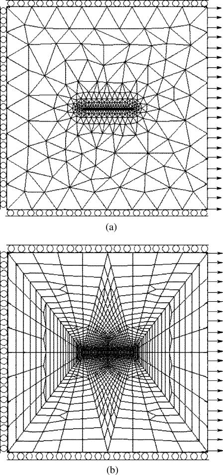
The tissues considered were thin membranes subjected to uniaxial in-plane stretching, which were modeled with plane stress conditions (Saada, 1993). Analyses all required a planar mathematical discretization of a region containing a prescribed number of cells with prescribed orientations (Figs. 1 and 2). Since some random distributions of cells required extensive statistical analyses, many different FE meshes were needed.

FIGURE 1.

Representative FE meshes used to calculate strain factors. (a) 1D cell discretization (thick lines denote cells) and (b) 2D cell discretization. The periodic boundary conditions represented a tissue that was infinitely long in the loading direction.

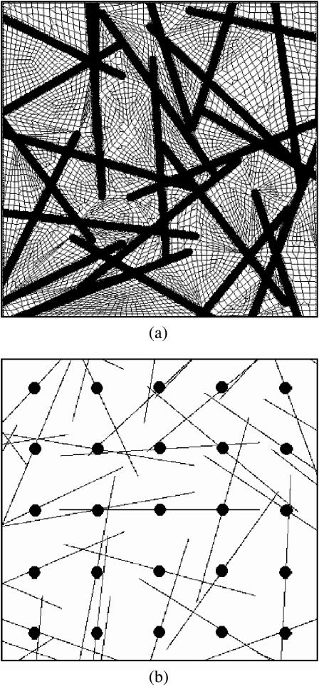
FIGURE 2.

In studies of randomly oriented cells, 7 × 7 array of randomly oriented but evenly spaced cells was cropped to yield a 5 × 5 array. Representative meshes are shown for analyses using (a) ADINA and (b) a finite element program written using MATLAB. Note that in the latter, the tissue was discretized into a uniform 200 × 200 grid; each black pixel represents a “cell” element, whereas each white pixel represents a “matrix” element. The circles superimposed on the cells in b show the uniform spatial distribution of the 5 × 5 array of cells.

Boundary conditions simulated a tissue that was infinitely long in the direction of the applied stretch, and constrained from contracting in the direction perpendicular to this applied stretch. As depicted in Fig. 1, the top and bottom edges of all FE meshes were restrained from moving vertically, the left edges were restrained from moving horizontally, and the right edges were constrained to remain vertical while displacing. All edges were free of shear tractions. Analogous periodic boundary conditions were used in simulations involving applied shear strains.

The cells and matrix were parametrically assigned linear elastic, isotropic material properties. The matrix was assigned a Poisson's ratio of ν = 0.49, as were the cells in simulations requiring this.

In the following sections, we describe the models for cells and their limitations; the model for cell distributions; the FE discretizations; and the specially written FE code we developed for large analyses.

Sparse cell populations

As is appropriate for the class of tissue constructs described in Wakatsuki et al. (2000), cells in ADINA analyses were modeled with one-dimensional (1D) elastic elements having no flexural rigidity (Fig. 1 a). The stiffness of these elements added to that of the matrix so that the effective modulus of the cells could be taken to be a parallel summation of the moduli E_c of the cells and E_m of the matrix (e.g., Gere and Timoshenko, 1984):

(5)

The thin lines in Fig. 1 a represent the boundaries of plane stress, linear elastic, and quadratic interpolation elements; the elements representing the ribbon cells are shown as thick solid lines. The boundary and loading conditions were as described above. The meshes needed to be finest in the vicinity of the largest gradients of strain, which occurred around the edges of the cells.

Models in which the cells occupied a 2D region with elastic modulus E_c were studied for comparison (Fig. 1 b). In these meshes, the cell was modeled with 2D elements like those of the matrix.

Convergence studies.

The primary challenge in attaining convergence stemmed from the singularities in the elastic problems considered here: the elasticity solutions for ribbon cells and rectangular cells embedded in an elastic matrix predict infinite matrix strains at the end of the cell. FE analyses inherently smooth end effects over an area that is on the order of the element size.

We refined FE meshes until further refinement showed no effect on the strain factor. Convergence studies indicated accuracy on the order of a few percent; error decreased as the ratio of the cell and matrix moduli approached 1. All strain factors calculated using the FE method are upper bounds. FE models overpredict stiffness when the discretization and interpolation schemes used in the solution cannot precisely replicate the analytical displacement field. Elements used for the cells performed better than those used for the matrix because of the relatively uniform strain fields in the cells. The net result was a larger underprediction of strain in the matrix than in the cell, resulting in an overprediction of the strain factor.

Dense cell populations

Percolation was studied in tissues containing high concentrations of randomly oriented cells. These studies involved FE models containing 3 × 3 and 5 × 5 arrays of cells (Fig. 2). In the sample ADINA mesh shown in Fig. 2 a, the thin lines again represent the borders of plane stress quadratic elements, and the thick lines indicate the positions of 1D elements that comprise the cells. Attention focused on the central cell to avoid boundary effects; the surrounding cells served as a random environment for the central cell.

The spatial and orientation distributions for cells were based upon those observed in bio-artificial tissue constructs by Zahalak et al. (2000). A uniform spatial distribution was adopted for the positions of the centers of the cells, as shown by the circles plotted over the midpoints of cells in Fig. 2 b. Cases with nonuniform spatial distributions of the cells, which would produce macroscopic inhomogeneities, were not considered. Cell orientations were assigned according to a uniform probability density function, which would ensure planar isotropy given a sufficiently large grid of cells.

Finite element code for dense cell populations and large tissue samples

A FE code was written using MATLAB to analyze strain factors in cases of very large cell concentrations, and very large arrays of randomly oriented cells. Well-established algorithms for linear elastic FE analysis were employed (Szabo and Babuska, 1991). The code was fully validated through comparison to exact solutions and ADINA analyses. Plane stress linear interpolation elements were used. The meshes were constrained and loaded in the same manner as the ADINA meshes, and careful convergence studies were undertaken.

The program provided rapid, automated discretization of meshes containing 2D cell discretizations, and highly efficient analysis of tissues with dense cell populations. Meshes consisted of uniform 200 × 200 arrays of elements. As shown in Fig. 2 b, elements crossed by cells were assigned the Young's modulus of the cells, whereas all others were assigned that of the matrix (square elements corresponding to cells are represented in Fig. 2 b as black pixels; white regions correspond to matrix elements). Note that portions of cells from beyond the 5 × 5 array of cells can be seen around the periphery of this mesh. Cells had a width equal to the grid size, which was chosen to produce a slender cell aspect ratio (length/width > 20).

Analytical predictions for strain factors

To establish how strain factors should scale, we developed a scaling law for the strain factor, calibrated it with Monte Carlo simulations, and validated it against both numerical simulations and Eshelby's solution. The scaling law was extended to high cell concentrations using the percolation model presented in the section “Percolation, and a model for high cell concentrations”.

Scaling model

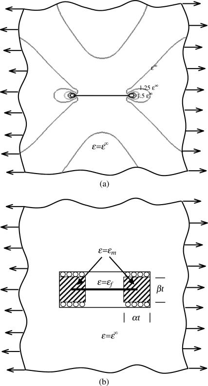
A scaling law was derived for tissues having a low cell concentration, meaning that cells were spaced sufficiently that the strain fields surrounding them did not interact appreciably. The scaling law was motivated by the strain field observed from FE analyses (Fig. 3 a). When the tissue receives a remote uniaxial strain ɛ_∞ (Fig. 3 a), the average axial strain within a relatively stiff cell is lower than ɛ_∞, whereas the matrix normal strain in the direction of the cell axis is greater than ɛ_∞ over a “region of influence” near the cell ends; if the matrix is more compliant that the cell, this will be reversed. The scaling model depicted in Fig. 3 b involved applying the equilibrium and the constitutive relations in the presence of an incompatible strain field (e.g., Hill, 1952). The tissue was divided into three regions, each having constant axial strain: 1), the cell, with axial strain ɛ_c; 2), regions of matrix connected to the ends of the cell with elevated or reduced axial strain ɛ_m; the size of these regions scale with the width t of the cell (αt × βt, where α and β are constants); and 3), matrix material unaffected by the cell, in which the axial strain equals the remote strain ɛ_∞.

FIGURE 3.

Schematic of the scaling model. (a) The strain field around a thin cell and (b) a cartoon showing the idealized strain field.

The force on the central linkage in Fig. 3 b must be the same for the “region of influence” and the cell. Using straightforward mechanics (e.g., Gere and Timoshenko, 1984), the force per unit depth F (out of the page) is

(6)

where β is the scaling constant shown in Fig. 3 b.

The condition that the total displacement Δ of this linkage must be in registry with that of the surrounding matrix with a constant strain ɛ_∞ may be written

(7)

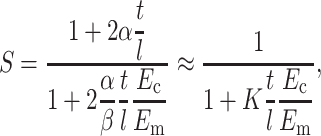
Equations 6 and 7 may be solved to obtain an expression for ɛ_c in terms of ɛ_∞. Then, the strain factor may be written as

(8)

where α, β, and K are scaling parameters, and the second expression is a good approximation for tissues whose cells have very high aspect (t/l ≪ 1). Considering that S = 1 when the cell-matrix modulus ratio is unity, we can see that β = 1. Note that Eq. 8 reduces to Eshelby's exact solution (Eq. 3) when the scaling parameter K = 2.

This scaling relationship and Eshelby's solution both suggest the following governing dimensionless parameter, which we call the normalized cell stiffness:

(9)

Percolation, and a model for high cell concentrations

The expressions for the strain factor in Eqs. 3 and 8 were derived for isolated cells. We extended these models to higher cell concentrations by 1), incorporating a statistical model for “effective cell length” that accounts for cell overlap and bonding, and 2), correcting the elastic properties of the matrix directly surrounding the cell to account for stiffening by neighboring cells.

Effective cell length.

The “effective cell length” increases when cells overlap. The average effective length for all cells was taken to be proportional to the average number of intersections per cell, as predicted with the Kallmes-Corte network model (Eq. 4). In a uniform, random distribution (eccentricity parameter e = 0) of N_c identical, slender cells (length l ≫ width t) spread over an area A_tissue, the average number of cell intersections N_i for each individual cell is

(10)

where the C = l² N_c/A_tissue is the 2D dimensionless cell concentration. C has the physical meaning of number of cells per unit area, normalized by the cell length. For a tissue of thickness h, containing ribbon cells of cross-sectional area A_c ≡ th, this is related to the number of cells per unit volume, N, by

(11)

Effective cell length increases with each cell intersection:

(12)

where the factor of 1/2 appears because each cell intersection is shared by two cells.

Effective matrix modulus.

As the cell concentration increases, the average stiffness of the material near each cell changes from the stiffness of the matrix. Using a self-consistent type approach (Budiansky, 1965; Hill, 1965), we modeled the matrix material surrounding each cell as having the effective elastic properties of the tissue as a whole. We used a “parallel” estimate for the effective modulus:

(13)

where E_c* is the contribution of the neighboring cells, which is greater than zero if the cells are stiffer than the matrix.

An expression for E_c* began by comparing a “real” tissue and a similarly sized membrane of pure matrix material. Both were subjected to a remote uniaxial strain in the 1-direction, with all other components of the remote strain tensor zero. Relating the two involved replacing each cell with a contractile force per unit depth, F, applied along each cell's axis. F is the force per unit depth that, when applied at each cell location in the membrane of pure matrix material, yields the strain field that occurs in the “real” tissue. This force is a function of the cell width, t, the axial cell strain, S, and the additional cell stiffness, (E_c − E_m):

(14)

E_c* is then the stiffening effect of these forces. For particular values of the dimensionless 2D cell concentration, C, cell length, l, and applied strain, , E_c* was found by averaging this force cell orientations, n_i (e.g., Bird et al., 1987):

(15)

where n₁ is the 1-component of the unit vector pointing along the axis of each cell. If θ is the angle between a cell's axis and the 1-direction, n₁ = cosθ. Substituting and assuming a uniform distribution of cell orientations,

(16)

Therefore,

(17)

Strain factor in dense cell concentrations.

Substituting Eqs. 12 and 17 into Eq. 9 yields an effective normalized cell stiffness:

(18)

reduces to Y_c at low cell concentrations. Inserting this into Eq.8 results in an expression for the strain factor that is valid for all cell concentrations, and captures the effect of percolation:

(19)

We call this generalization of the scaling model a “percolation model”.

Extension of the Zahalak model to incorporate strain factors

We extended the general three-dimensional Zahalak constitutive law to incorporate strain factors, and then specialized the law to 2D. The updated model was found by correcting the mean strain in the cells: , where S = S(Y_c,C) is the strain factor. One way to correct the equation for cell behavior is to incorporate this corrected strain into the final term:

(20)

Our approach was to redefine κ and ω, and continue to use the form in Eq. 1. The updated forms of Eq. 2 for relating κ and ω to cell moduli are then

(21)

Using Eqs. 11 and 21, these can be specialized to the 2D case

(22)

where the superscripts 0 and ∞ refer to the instantaneous and long-term responses of the tissue constituents, respectively.

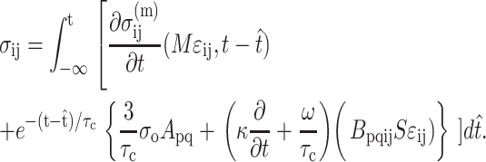
The factors that reduce the average strain in the cells also amplify the average strain in the matrix. As derived in Appendix B, the strain in the matrix is amplified by the factor M:

where , in which v_c is the volume of a cell. As discussed in Appendix B, this must be accounted for in the matrix stress terms in the modified Zahalak constitutive model:

Updated framework for determining cell stiffness from measured parameters

N, l, h, , and can be found from calibration experiments; the parameters κ and ω are obtained from direct measurements on a tissue. The elastic modulus of cells is found by 1), using Eq. 11 to calculate C; 2), using Eq. 22 to calculate Y_cS; 3), determining Y_c from the characteristic relationship between Y_c and Y_cS described in the section "Cell stiffness predicted by the modified 2D Zahalak model, and 4), using Eq. 9 to calculate the cell modulus E_c from Y_c.

RESULTS

Numerical simulations were needed to calibrate and validate the analytical, scaling, and statistical models used in this work. We begin in the next section with a validation and assessment of the concept of a strain factor in cases that extend beyond those explicitly allowed by Eshelby's exact solution, and a Monte Carlo calibration of the fitting parameter K.

The statistical extension of the scaling model to tissues with dense cell populations (the section “Percolation, and a model for high cell concentrations”) was validated against numerical approximations to exact continuum mechanics solutions. The Monte Carlo simulations presented in the section “Strain factors in random arrays of cells” show that the percolation model captures the mechanics of interacting cells correctly, and accurately predicts the cell concentration corresponding to and mechanical consequences of the formation of a continuous, “percolated” network of cells.

The validated and calibrated scaling and percolation models were inserted into the updated Zahalak constitutive model and used to generate a chart needed to interpret cell properties from the results of tests on tissue constructs. This chart is presented in the section “Cell stiffness predicted by the modified 2D Zahalak model”, and used to reinterpret experimental results presented by Zahalak et al. (2000).

Strain factors in nonellipsoidal cells

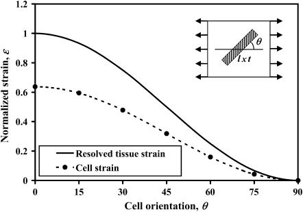
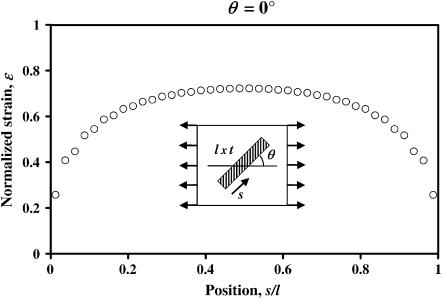
Eshelby's exact solution shows that the strain factor is mathematically rigorous for isolated, aligned, arrays of ellipsoidal cells. We begin with an assessment of strain factors in nonellipsoidal cells. Strain factors were evaluated numerically for a series of model tissues strained as in Fig. 1. Sample data corresponding to a 1D cell discretization (length = l, cell spacing = 4 l, t = 0.05 l, E_c/E_m = 5) is shown in Fig. 4. For all of the results presented, strains are normalized by the magnitude of the maximum remote principal strain. The solid curve represents the normalized macrostrain, resolved in the direction of a cell; circles represent the normalized average longitudinal strain in the cell. The key result is that the two curves are proportional, regardless of the cell orientation angle. As shown in Table 1 a, the strain factor, which is the constant of proportionality between the two curves, is very nearly constant for all cell orientations. Table 1 b shows strain factors for the same model tissue, now loaded with a remote shear strain. The strain factors were again independent of cell orientation, and were very close those calculated for uniaxial loading.

FIGURE 4.

Cell strain and macrostrain versus cell angle, θ, in a periodic array of aligned cells. The solid line represents the average tissue strain (macrostrain) resolved in the direction of the cell; the circles are the longitudinal cell strains predicted by FE calculations. The constant of proportionality relating the two curves is the “strain factor”.

TABLE 1.

Strain factors as a function of cell orientation

(a) Axial stretching
Orientation	Strain factor 90%	Strain factor 100%
0°	0.659	0.632
15°	0.660	0.633
30°	0.662	0.636
45°	0.664	0.638
60°	0.668	0.642
75°	0.670	0.644
Average	0.664	0.637
Standar Deviation	0.005	0.005
(b) Shearing deformation
Orientation	Strain factor 90%	Strain factor 100%
15°	0.657	0.625
30°	0.659	0.627
45°	0.662	0.631
60°	0.668	0.637
75°	0.684	0.650
Average	0.666	0.634
Standard Deviation	0.011	0.010

For the second column, we average the strain in a cell using 90% of its length; for the third, we use its whole length.

(a) Uniaxial stretching of a tissue; (b) shearing.

Fig. 5 shows that the axial strain distribution is not uniform in nonellipsoidal cells, with the majority of the nonuniformity concentrated near the cell ends. Table 1, a and b, show that this effect is small: the difference between the strain factor averaged over the entire cell length, and that calculated over 90% of the cell length, is on the order of 5%, meaning that the strain factor provides a reasonable approximation of the mean axial cell strain.

FIGURE 5.

Axial strain in a cell is fairly uniform, except near the cell's ends.

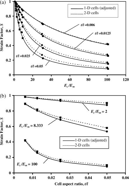
An aspect we explored carefully was the 1D cell discretization. Fig. 6 shows that the 1D and 2D cell discretizations (Fig. 1 b) show reasonable agreement: Fig. 6 a shows that the agreement is best for modulus ratios E_c/E_m near 1 for all cell shapes, and Fig. 6 b shows that the agreement is also very close when the cell aspect ratio t/l is very small and E_c/E_m is very large. Each point on the curves represents the average strain factor calculated from analyses of cells pointing at angles of 0°, 15°, 30°, 45°, 60°, and 75° from the principal straining direction. The 1D case for Fig. 6 b contains values interpolated from Fig. 6 a. The elastic modulus used for the 1D simulations is from Eq. 4 (note that since the 1D discretization involves superimposing cell and matrix stiffness, cases in which the cell is more compliant than the matrix could not be captured with a 1D discretization).

FIGURE 6.

A study of how the cell discretization scheme affects predictions of the strain factor. The 1D and 2D discretization schemes are closest for tissues with (a) very small and large modulus ratios E_c/E_m and (b) small cell aspect ratios t/l.

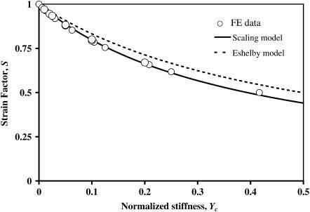
Monte Carlo analyses involving 21 sets of FE analyses showed that the form of the scaling law in Eq. 8 is correct at low cell concentrations. As predicted, all data for strain factors collapsed to a single curve when plotted against Y_c = t/l E_c/E_m (Fig. 7); the scaling model of Eq. 8 best fit the data with K = 2.2. The results shown with circles are for tissues with cell spacing b = 4 l, with all permutations of t/l = {0.006,0.01,0.0125,0.025,0.05} and E_c/E_m = {2,5,8.33}. Additionally, results are shown for b = 2 l, t/l = 0.01, and E_c/E_m = {2,5,10,20}. Eshelby's solution (Eq. A6) followed the FE data fairly well, especially at very low values of t/l, but consistently overpredicted the strain factor.

FIGURE 7.

Validation of the scaling law at low cell density. Numerical estimates of strain factors are plotted with circles. Eshelby's solution and the scaling law both match the FE simulations qualitatively.

Strain factors in random arrays of cells

A second limitation of the Eshelby and scaling models for the strain factor is that they are derived for aligned cells. To verify that the concept of a strain factor is valid in tissues with nonaligned distributions of cells, we studied strain factors in randomly oriented cells in a square 3 × 3 array of cells. We calculated the average strain at the central cell in the 3 × 3 array, which was oriented at an angle θ from the direction of stretching and surrounded by eight randomly oriented cells. The results followed the cos²θ distribution as in Fig. 4.

Strain factors in dense cell populations

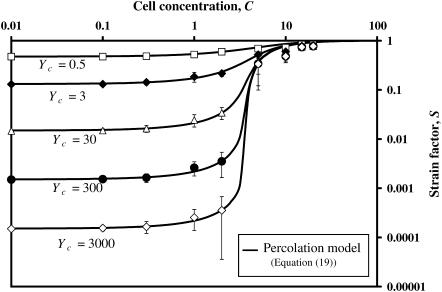
To validate the statistical “percolation” model (Eq. 18) that extends the scaling model to higher cell concentrations, a series of Monte Carlo simulations of 5 × 5 arrays of cells (Fig. 2) were run. As shown in Fig. 8, the percolation model (Eq. 18) predicts all features of the results for the parameter range shown. The model is highly accurate at low and medium cell concentrations, and a good approximation at very high cell concentrations. The Eshelby model (not shown) predicted the lower asymptotes of the curves to within a few percent.

FIGURE 8.

FE predictions of the strain factor as a function of cell concentration. Also plotted is the percolation model, which predicts the cell concentration at which network formation leads to a sharp increase in the strain factor.

Each point in Fig. 8 for C < 1 corresponds to an average of two analyses using ADINA; since the cells were nearly isolated, the scatter was extremely small. The remaining points each represent the average of 20 analyses using the specially written FE program (the section “Finite element code for dense cell populations and large tissue samples”); the 10-fold increase in the number of analyses was necessitated by the increase in scatter that occurred at cell concentrations near the “percolation point”. This scatter is evident from the increase in the size of the error bars near a concentration of C = 3 (Fig. 8); relative scatter was highest for intermediate numbers of cell intersections.

Cell stiffness predicted by the modified 2D Zahalak model

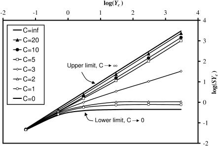
The central result of this article, needed for interpreting experiments on tissue constructs, is the relation between log(Y_cS) and log(Y_c), shown in Fig. 9. These curves were derived from the fitted percolation model (Eq. 19). The “upper limit” curve was established by noting that as the cell concentration grows, S approaches 1, and log(Y_cS) approaches log(Y_c). The “lower limit” curve was established from Eq. 19 by noting that as Y_c increases, log(Y_cS) asymptotes to log(1/K).

FIGURE 9.

Relationship between the normalized stiffness, Y_c, and the product SY_c, which can be found from experimental measurements. This plot is needed to derive in situ cell stiffness from macroscopic tissue measurements. The Zahalak model corresponds to the upper limit.

Zahalak et al. (2000) reported values for the short-time and long-time cell moduli at different strain levels. Their tissue constructs were a “borderline” 2D case (the remodeled tissue thickness was on the order of 2–3 cell widths), which we modeled as 2D.

Applying the procedure described in the section “Updated framework for determining cell stiffness from measured parameters” to reinterpret their experiments, we arrived at the data listed in Table 2. The elastic modulus used for the matrix was the tangent modulus estimated for a nominal strain of 3%. The average short-term cell modulus predicted by the modified theory was 10-fold higher than that predicted by Zahalak et al. (2000), whereas the long-term cell modulus response was of the same order of magnitude. This result can be explained in terms of the relative stiffnesses of the cell and matrix, as discussed below.

TABLE 2.

Cell stiffness calculated using the unmodified Zahalak model, compared to those calculated using the modified theory

	Cell and matrix stiffness
	(Ec/Em)∞	(Ec/Em)0	(Ec)∞[MPa]	(Ec)0[MPa]
Zahalak's model	21 ± 15	73 ± 32	0.09 ± 0.054	0.62 ± 0.22
Modified theory	35 ± 26	124 ± 54	0.15 ± 0.09	1.06 ± 0.37

The moduli used for the matrix were based on those reported by Zahalak et al. (2000), and were estimated as the tangent moduli for a nominal matrix of 3%: (E_m)_o = 8.5 kPa, and (E_m)_∞ = 4.3 kPa.

DISCUSSION

A fundamental assumption of the Zahalak constitutive model was overcome in this article by incorporating a more accurate assessment of the average strain experienced by cells in a tissue. The quantity we call the strain factor relates the remote strain tensor to the average strain in cells.

Strain factors are properties of a tissue

Eshelby's exact solution shows that a strain factor is an intrinsic property for tissues containing isolated, aligned, elliptical cells. We have shown that this is also a reasonable approximation for arbitrarily dense populations of randomly oriented ribbon-shaped cells, and derived models that predict the strain factor based upon a parametric description of a tissue.

At dimensionless cell concentrations of C > 1, cells can intersect and bond with one another; the average number of cell crossings increases with C, as predicted by Eq. 4. At these higher cell concentrations, interaction and bonding between cells leads to an increase in the average strain factor within a tissue. This also leads to a broader distribution of strain factors throughout a tissue. Although we cannot predict this distribution, the ensemble average represented by Eq. 19 is appropriate for the Zahalak model, which is based on statistical averaging of cell force components.

At even higher cell concentrations, the cells form a continuous network, and the cell strain approaches the tissue strain; consequently, the strain factor approaches 1. The percolation point is evident as a jump in Fig. 8 at a C = 3.5–4, and is modeled very accurately by the percolation model. The percolation point is independent of mechanical properties of the tissue constituents. Since tissues with very stiff cells (high Y_c) have lower strain factors at subpercolation cell concentrations, the magnitude of the percolation jump increases as Y_c increases, leading to a relatively sharper percolation threshold in Fig. 8.

Analytical predictions of strain factors

The scaling model in this article was found to predict strain factors lower than those predicted by Eshelby's exact solution for elliptical cells. The difference stems from the fact that the cross-sectional area of elliptical cell varies along the cell length, whereas the ribbon cells have a uniform cross section (Steif and Hoysan, 1987). When comparing the models, the stiffnesses were set equal at the center points of the cells. Strain factors calculated by Eshelby's theory were greater than those predicted by the FE calculations, because of the extra compliance along the remainder of the elliptical cells.

Modification of the Zahalak model

The update to the Zahalak model includes a corrected average strain field for cells distributed in a 2D planar isotropic fashion. For the thin constructs studied by Zahalak et al. (2000), the 2D plane-stress theory was justified. However, more work is needed to extend the updated model to include tissues where cell orientation distributions contain a significant out-of-plane component. Our work is applicable only to the very long-term and very short-term mechanical response of a tissue. Future studies involving the time-dependence of the strain factor are needed to extend this work to loading situations in which viscous components of mechanical response are important. Finally, material nonlinearity is an important extension that must be addressed in future work.

The Zahalak model underpredicts cell stiffness for cases in which the strain factor is not unity (Table 2). The discrepancy is greater in the short-term response of the tissue than in the long-term response. This is expected, since the cell stiffness for the short-term response is much higher than the matrix stiffness, whereas the stiffnesses are much closer for the long-term response. This means that the strain factor is farther from 1 for the short-term response than for long-term response.

Estimates of cell stiffness

The fully relaxed elastic modulus for fibroblasts presented is slightly higher than most reported by others using four different techniques (Table 3). Two factors make comparison among these experiments difficult, however.

TABLE 3.

Values of cell modulus estimated by different state-of-the-art techniques vary widely; relaxed elastic cell modulus estimated by different approaches

Technique	References	Elastic modulus (MPa)
Micropipette aspiration	Guilak et al. (1999)	0.0002–0.004
	Miyazaki et al. (1999)	0.10
Magnetic tweezers	Bausch et al. (1999)*	0.0006–0.002
Torsion of ferromagnetic beads	Bausch et al. (1998)	0.04–0.12
	Fabry et al. (2001)	0.0001–0.01
Cell-poking	Petersen et al. (1982)	0.015
Laser tracking microrheology	Yamada et al. (2000)	0.00001–0.001
AFM cell-poking	Hoffman et al. (1997)*	0.005–0.2
	Mahaffy et al. (2000)	0.002–0.008
	Mahaffy et al. (2004)	0.0019–0.0024
2D tissue constructs	Reinterpretation of data from Zahalak et al. (2000)	Instantaneous: 1.2
			Fully relaxed: 0.15

The relationship between these estimates is unclear, due to the radically different ways in which cells are loaded in each case. Entries marked with an asterisk are estimates of the properties of specific cell constituents, rather than estimates of overall cell moduli. When converting data to Young's moduli, a Poisson's ratio ν = 0.5 was used in conjunction with an assumption of isotropy.

First, cells are not linear elastic solids: their continuum response varies with strain (Wakatsuki et al., 2000). Since none of these other techniques produces constant strain fields, comparison to these results is difficult.

Second, the meaning of an elastic modulus is different in the four experiments. The stiffness we estimate is the continuum stiffness contribution of a cell subjected to uniform straining of a particular level. This has a different meaning than the cell modulus estimated by a shear traction applied to the outermost membrane (as with magnetic tweezers and torsion of ferromagnetic beads), where the mechanism of load transfer to the cytoskeleton is uncertain. The elastic modulus estimated by applying localized indentations to the cell membrane (as with cell-poking) varies depending on the specific location of indentation (Petersen et al., 1982), and localized buckling of microstructural features can lead to underprediction of the stiffness. The high strains (∼1) involved micropipette aspiration of cells involve microstructural cell changes that are difficult to characterize. The relationships between moduli estimated by these different methods need to be explored more fully.

Our reinterpretation of results in Zahalak et al. (2000) indicate that the instantaneous moduli of cells are an order of magnitude stiffer than the fully relaxed moduli (Table 3). This is consistent with atomic force microscopy cell-poking results of Mahaffy et al. (2000), who find that the high frequency response of cells is an order of magnitude stiffer than the low-frequency response. However, as mentioned above, direct comparison between techniques involving highly nonuniform strain fields and those involving uniform strain fields is tenuous.

CONCLUSION

The modified theory presented in this article provides an improvement to the accuracy of predictions of cell stiffness in bio-artificial tissue constructs.

The article showed that a strain factor is a reasonably accurate approach to predicting the strain experienced by cells as a function of overall tissue strains.

After obtaining the strain factor for a wide range of tissue properties (cell concentration and normalized stiffness), we developed a method for determining the cell stiffness as a function of easily measured properties of a tissue. A chart based upon the models in this article must be consulted in this analysis. We conclude that applying Zahalak's model with an assumed strain factor of 1 leads to errors that can be an order of magnitude in certain cases.

The 2D theory in this article can be used to more accurately predict in situ cell short-term and long-term stiffness in thin bio-artificial tissues. However, further work is needed to extend this approach to cases in which cell distributions contain a significant out-of-plane component, cases in which material nonlinearity is important, and cases in which rate-dependent properties are desired.

APPENDIX A: EXPRESSIONS FOR STRAIN FACTOR USING ESHELBY'S THEORY

Eshelby's (Eshelby, 1957, 1959) solution is a fundamental tool for the analysis of composite materials (e.g., Fukuda and Kawata, 1974; Fukuda and Chou, 1982). We apply it here to provide an exact solution for the strain factor in the special case of an isolated ellipsoidal cell aligned with the direction of macroscopic straining. The tissue is modeled as an initially stress-free, homogeneous, infinite continuum with matrix stiffness tensor C^(m) (e.g., Saada, 1993), and the cell is modeled as a region within this continuum that is removed, then subjected to a stress-free “transformation strain” (“eigenstrain”) ɛ^(c) that requires no surface traction (note that boldface variables indicate tensors of nonzero rank). Rebonding the cell to the matrix requires a strain field ɛ^(r) in the infinite continuum. The corresponding stress field σ^(m) within the matrix at a position x is σ^(m)(x) = C^(m)ɛ^(r)(x), and the uniform stress within the cell can be written as σ^(c) = C^(m)(ɛ^(r) − ɛ^(t)). Eshelby showed that the uniform strain ɛ^(r) needed for rebonding the cell is related to the eigenstrain ɛ^(t) by the expression ɛ^(r) = Eɛ^(t), where E is called the Eshelby tensor.

Eshelby's approach also applies to the case when the cell has a stiffness tensor C^(c) different from of the matrix. This involves comparing the “real” tissue, containing a cell that undergoes no eigenstrain, to a homogeneous “comparison” tissue with a cell-shaped region subjected to an eigenstrain ɛ^(t). Both tissues are subjected to a uniform applied strain field at infinity, ɛ^(∞). The key is to find the eigenstrain ɛ^(t) that produces the same stress and strain fields in both tissues. For the “real” tissue, the stress in the cell is σ^(c) = C^(c)ɛ^(c) = C^(c)(ɛ^(∞) + ɛ^(r)); for the “comparison” tissue, σ^(c) = C^(m)(ɛ^(∞) + ɛ^(r) − ɛ^(t)). Equating these two expressions, recalling that ɛ^(r) = Eɛ^(t), noting that for isolated cells the average tissue strain is ɛ^(a), and rearranging some terms, we obtain

(A1)

where A^Eshelby = [I + E(C^(m))⁻¹(C^(c) − C^(m))]⁻¹ is the strain-concentration tensor. Note that the unit tensor is defined as I_ijkl = 1/2 (δ_ik δ_jl + δ_il δ_jk), in which the Kronecker delta δ_ij is unity when the value of the index i equals that of the index j, and zero otherwise.

This relationship between cell and tissue strain can be used to predict the strain factor. For planar isotropic tissue constructs (e.g. Wakatsuki et al., 2000), C^(c) and C^(m) can be written in terms of the Young's modulus E and Poisson's ratio ν of the cells and matrix, {E_c,ν_c} and {E_m,ν_m}, respectively (Saada, 1993). A^Eshelby can be written in terms of the elastic constants and the dimensions t and l of the cell's in-plane axes (e.g., Mura, 1982). For a tissue subjected to a remote uniform axial strain in the 1-direction, with all other components of the remote strain tensor ɛ^(∞) zero, the strain factor S in a cell pointed along the unit vector n is

(A2)

Substituting into expressions available in Mura (1982) for the Eshelby tensor, E, the general expression for strain factor S of 2D elliptical cells can be written in closed form as

(A3)

where t_l is the aspect ratio t/l, and m is Young's modulus ratio E_c/E_m. For ν_c = ν_m = ν, and neglecting terms of order and higher, we have,

(A4)

When ν = 0, strain factor becomes,

(A5)

And, when ν = 0.5, the strain factor simplifies to

(A6)

APPENDIX B: MATRIX-CORRECTED STRAIN AND STRESS

The constitutive model in this article considers the contributions of the cells and the matrix independently. However, the two are coupled: stiff cells amplify the average strain in the matrix, whereas compliant cells reduce it. We quantified this effect by considering the average strain ɛ_ij in a control volume of a tissue, which is the weighted sum of the average strains in the cells and matrix:

(B1)

where the cell volume fraction f_c is fraction of the volume that is occupied by cells. In terms of the cell concentration, N, and the average volume v_c occupied by an individual cell,

(B2)

Since the average cell strain is given by S ɛ_ij,

(B3)

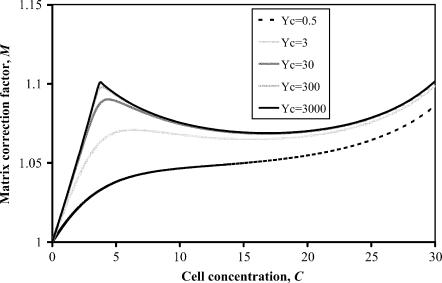
The variation of M as a function of normalized stiffness Y_c and dimensionless concentration C is shown graphically in Fig. 10. The average matrix strain increases up to the percolation point (C ≈ 3.5), then drops slightly. The net increase in the average matrix strain is smallest for thin cells (t/l < 20). Equation B3 is not valid for extremely high cell concentrations, since the relationship in Eq. B2 does not account for the details of cell overlap. As a consequence, Eq. B3 predicts that M approaches infinity as the cell volume fraction approaches 1; in fact, the Eshelby solution predicts that M should approach an upper limit of 2.5–3.0 for cases when the matrix stiffness is much smaller than the cell stiffness, and the small remaining pockets of matrix material can be approximated as ellipsoidal in shape.

FIGURE 10.

Amplification of average matrix strain as a function of cell concentration and normalized stiffness.

References

- Bachrach, N. M., W. B. Valhmu, E. Stazzone, A. Ratcliffe, W. M. Lai, and V. C. Mow. 1995. Changes in proteoglycan synthesis of chondrocytes in articular cartilage are associated with the time-dependent changes in their mechanical environment. J. Biomech. 28:1561–1569. [DOI] [PubMed] [Google Scholar]
- Baer, A. E., and L. A. Setton. 2000. The micromechanical environment of intervertebral disc cells: Effect of matrix anisotropy and cell geometry predicted by a linear model. J. Biomech. Eng. 122:245–251. [DOI] [PubMed] [Google Scholar]
- Bausch, A. R., F. Ziemann, A. A. Boulbitch, K. Jacobson, and E. Sackmann. 1998. Local measurements of viscoelastic parameters of adherent cell surfaces by magnetic bead microrheometry. Biophys. J. 75:2038–2049. [DOI] [PMC free article] [PubMed] [Google Scholar]
- Bausch, A. R., W. Moller, and E. Sackmann. 1999. Measurement of local viscoelasticity and forces in living cells by magnetic tweezers. Biophys. J. 76:573–579. [DOI] [PMC free article] [PubMed] [Google Scholar]
- Bird, B. R., C. F. Curtiss, R. C. Armstrong, and O. Hassager. 1987. Dynamics of Polymeric Liquids, Vol. 2. Kinetic Theory. Wiley, New York.
- Budiansky, B. 1965. On the elastic moduli of some heterogeneous materials. J. Mech. Phys. Solids. 13:223–227. [Google Scholar]
- Budiansky, B., and Y. L. Cui. 1995. Toughening of ceramics by short aligned fibers. Mech. Mater. 21:139–146. [Google Scholar]
- Chou, T. W. 1992. Microstructural Design of Fiber Composites. Cambridge University Press, Cambridge, UK.
- Eshelby, J. D. 1957. The determination of the elastic field outside an ellipsoidal inclusion, and related problems. Proc. Roy. Soc. A. 241:376–396. [Google Scholar]
- Eshelby, J. D. 1959. The elastic field outside an ellipsoidal inclusion. Proc. Roy. Soc. A. 252:561–569. [Google Scholar]
- Fabry, B., G. N. Maksym, J. P. Butler, M. Glogauer, D. Navajas, and J. J. Fredberg. 2001. Scaling the microrheology of living cells. Phys. Rev. Lett. 87:148102-1–148102-4. [DOI] [PubMed] [Google Scholar]
- Fukuda, H., and T. W. Chou. 1982. A probabilistic theory of the strength of short-fibre composites with variable fibre length and orientation. J. Mater. Sci. 17:1003–1007. [Google Scholar]
- Fukuda, H., and K. Kawata. 1974. On Young's modulus of short fiber composites. Fibre Sci. Technol. 7:207–222. [Google Scholar]
- Fung, Y. C. 1981. Biomechanics: Mechanical Properties of Living Tissues. Springer-Verlag, New York.
- Guilak, F., W. R. Jones, H. P. Ting-Beall, and G. M. Lee. 1999. The deformation behavior and mechanical properties of chondrocytes in articular cartilage. Osteoarthritis Cartilage. 7:59–70. [DOI] [PubMed] [Google Scholar]
- Guilak, F., and V. C. Mow. 2000. The mechanical environment of the chondrocyte: a biphasic finite element model of cell-matrix interactions in articular cartilage. J. Biomech. 33:1663–1673. [PubMed] [Google Scholar]
- Gere, J. M., and S. P. Timoshenko. 1984. Mechanics of Materials, 2nd ed. PWS Publishers, Boston.
- Hill, R. 1950. The Mathematical Theory of Plasticity. Clarendon Press, Oxford.
- Hill, R. 1965. A self-consistent mechanics of composite materials. Mech. Phys. Solids. 13:213–222. [Google Scholar]
- Hofmann, U. G., C. Rotsch, W. J. Parak, and M. Radmacher. 1997. Investigating the cytoskeleton of chicken cardiocytes with the atomic force microscope. J. Struct. Biol. 119:84–91. [DOI] [PubMed] [Google Scholar]
- Kallmes, O., and H. Corte. 1960. The structure of paper: the statistical geometry of an ideal two-dimensional fiber network. Tappi. 43:737–752. [Google Scholar]
- Mahaffy, R. E., C. K. Shih, F. C. MacKintosh, and J. Käs. 2000. Scanning probe-based frequency-dependent microrheology of polymer gels and biological cells. Phys. Rev. Lett. 85:880–883. [DOI] [PubMed] [Google Scholar]
- Miyazaki, H., Y. Hasegawa, and K. Hayashi. 1999. Tensile property of fibroblasts from the rabbit patellar tendon. ASME Bioengineering Conference, Big Sky, MT.
- Mow, V. C., and A. Ratcliffe. 1997. Structure and function of articular cartilage and meniscus. In Basic Orthopaedic Biomechanics, 2nd ed. V. C. Mow and W. C. Hayes, editors. Lippicott-Raven Publishers, Philadelphia, PA.
- Mura, T. Micromechanics of Defects in Solids. 1982. Martinus Nijhoff, The Hague, The Netherlands.
- Ozerdem, B., and A. Tozeren. 1995. Physical response of collagen gels to tensile strain. J. Biomech. Eng. 117:397–401. [DOI] [PubMed] [Google Scholar]
- Parry, D. A. D. 1988. The molecular and fibrillar structure of collagen and its relationship to the mechanical properties of connective tissue. Biophys. Chem. 29:195–209. [DOI] [PubMed] [Google Scholar]
- Petersen, N. O., W. B. McConnaughey, and E. L. Elson. 1982. Dependence of locally measured cellular deformability on position on the cell, temperature, and cytochalasin B. Proc. Natl. Acad. Sci. USA. 79:5327–5331. [DOI] [PMC free article] [PubMed] [Google Scholar]
- Pins, G. D., E. K. Huang, D. L. Christiansen, and F. H. Silver. 1997. Effects of static axial strain on the tensile properties and failure mechanisms of self-assembled collagen fibers. J. Appl. Polym. Sci. 63:1429–1440. [Google Scholar]
- Prager, W. 1969. On the formulation of constitutive equations for living soft tissues. Q. Appl. Math. 27:128–132. [Google Scholar]
- Pryse, K. M., A. Nekouzadeh, G. M. Genin, E. L. Elson, and G. I. Zahalak. 2003. Incremental mechanics of collagen gels: new experiments and a new viscoelastic model. Ann. Biomed. Eng. 31:1287–1296. [DOI] [PubMed] [Google Scholar]
- Roeder, B. A., K. Kokini, J. E. Sturgis, J. P. Robinson, and S. L. Voytik-Harbin. 2002. Tensile mechanical properties of three-dimensional type i collagen extracellular matrices with varied microstructure. J. Biomech. Eng. 124:214–222. [DOI] [PubMed] [Google Scholar]
- Saada, A. S. 1993. Elasticity: Theory and Applications. Krieger Publishing, Melbourne, FL.
- Steif, P. S., and S. F. Hoysan. 1987. An energy method for calculating the stiffness of aligned short-fiber composites. Mech. Mater. 6:197–210. [Google Scholar]
- Szabo, B., and I. Babuska. 1991. Finite Element Analysis. Wiley, New York.
- Tucker, C. L., and E. Liang. 1999. Stiffness prediction for unidirectional short-fiber composites: review and evaluation. Comp. Sci. Tech. 59:655–671. [Google Scholar]
- Yamada, S., D. Wirtz, and S. C. Kuo. 2000. Mechanics of living cells measured by laser tracking microrheology. Biophys. J. 78:1736–1747. [DOI] [PMC free article] [PubMed] [Google Scholar]
- Wakatsuki, T., M. S. Kolodney, G. I. Zahalak, and E. L. Elson. 2000. Cell mechanics studied by a reconstituted model tissue. Bioph. J. 79:2353–2368. [DOI] [PMC free article] [PubMed] [Google Scholar]
- Wu, J. Z., and W. Herzog. 2000. Finite element simulation of location- and time-dependent mechanical behavior of chondrocytes in unconfined compression tests. Ann. Biomed. Eng. 28:318–330. [DOI] [PubMed] [Google Scholar]
- Wu, J. Z., W. Herzog, and M. Epstein. 1999. Modelling of location- and time-dependent deformation of chondrocytes during cartilage loading. J. Biomech. 32:563–572. [DOI] [PubMed] [Google Scholar]
- Zahalak, G. I., J. E. Wagenseil, T. Wakatsuki, and L. E. Elson. 2000. A Cell-based constitutive relation for bio-artificial tissues. Biophys. J. 79:2369–2381. [DOI] [PMC free article] [PubMed] [Google Scholar]