

Abstract
We provide evidence that the onset of functional dynamics of folded proteins with elevated temperatures is associated with the effective sampling of its energy landscape under physiological conditions. The analysis is based on data describing the relaxation phenomena governing the backbone dynamics of bovine pancreatic trypsin inhibitor derived from molecular dynamics simulations, previously reported by us. By representing the backbone dynamics of the folded protein by three distinct regimes, it is possible to decompose its seemingly complex dynamics, described by a stretch exponential decay of the backbone motions. Of these three regimes, one is associated with the slow timescales due to the activity along the envelope of the energy surface defining the folded protein. Another, with fast timescales, is due to the activity along the pockets decorating the folded-state envelope. The intermediate regime emerges at temperatures where jumps between the pockets become possible. It is at the temperature window where motions corresponding to all three timescales become operative that the protein becomes active.
INTRODUCTION
Understanding the temperature dependence of the internal motions in folded proteins is essential for controlling the function of biological molecules, as well as designing new systems with diverse properties. Recently, a substantial amount of experimental (Daniel et al., 1998; Fenimore et al., 2002; Pal et al., 2002; Tsai et al., 2001; Zaccai, 2000) and theoretical (Baysal and Atilgan, 2002; Dvorsky et al., 2000; Tarek and Tobias, 2002; Tournier et al., 2003; Vitkup et al., 2000) research effort has been invested in this direction. It has now been established that the protein and a solvent shell of thickness ∼4 Å (Dastidar and Mukhopadhyay, 2003) constitute the system of interest (Tarek and Tobias, 2002). An essential part of the overall motion of this system is slaved to the bulk solvent, implying that the enthalpic and entropic contributions to the free energy fluctuations in the protein originate in the solvent and the protein-hydration shell system, respectively (Fenimore et al., 2002). Investigations on the temperature-dependent properties of folded proteins reveal that hydrated proteins show a dynamical transition above which temperature they are active (Zaccai, 2000). Experimentally, the transition temperature is quantified by, e.g., monitoring the average fluctuations of hydrogen atoms in neutron scattering. Typical temperatures studied range from well below the transition region (observed at ∼190–220 K for different proteins) to right below unfolding. The fluctuations are anharmonic even at temperatures as low as 100 K (Hayward and Smith, 2002). In dehydrated powder samples or for samples in solvents that do not permit functionality, the fluctuation amplitude increases linearly throughout the temperature window studied. In other samples, the slope shows an increase during the transition temperature and attains a larger value at physiological temperatures.
It has been argued that the dynamical transition is controlled by the solvent (Caliskan et al., 2003; Tsai et al., 2001; Zaccai, 2003). For example, heat capacity measurements in the temperature range of 8–300 K on hen egg-white crystals with varying water content suggest that the observed transition behavior is a result of cooperativity in the system composed of the protein and the shell of water around the protein (Miyazaki et al., 2000). Yet, more recently, Halle has pointed to the effect of cooling rate on the distribution of conformational states at low temperatures using a two-state model of the protein (Halle, 2004). Thus, it is far from clear how the solvent affects the landscape, and which processes are onset with increasing temperature. A detailed understanding of the energy landscape of complex molecular systems, such as proteins, requires the investigation of their dynamics through simulations and models.
That the relaxation behavior of the mean square fluctuations of the atomic coordinates display nonexponential decay has been shown using molecular dynamics (MD) simulations on crambin and cytochrome c (Garcia et al., 1997; Garcia and Hummer, 1999). Recently, we have also studied the relaxation phenomena related to the backbone dynamics of bovine pancreatic trypsin inhibitor (BPTI) in the folded state by analyzing results from extensive MD simulations spanning a wide temperature window (Baysal and Atilgan, 2002). Therein we have shown, by analyzing the backbone dynamics, that relaxation of the internal motions display extensive coupling. However, very little has been said on the nature of this coupling. In particular, a marked change in backbone dynamics with the onset of functional dynamics over a temperature window of ∼30 K was noted. It was suggested that different relaxation phenomena are invoked, probably in a hierarchical manner, as the temperature increases.
To gain insight into the processes involved, we study the equilibrium fluctuations and the relaxation phenomena of the fluctuation vector attached to the Cα atoms of the BPTI. We confine our attention to the protein-water system, and we utilize MD simulations in the temperature range spanning 150–320 K, where the results correspond to infinitely fast cooling. We find that it is possible to explain the observed phenomena through a simplistic view of protein dynamics, where insertion of a new characteristic timescale between that of the rapid fluctuations of the atoms and the slow-mode motions of the overall system occurs. The latter are present at temperatures even well below those corresponding to the physiologically active protein. We propose that these intermediate timescales belong to processes that control conformational jumps between the rotameric states of side-chain dihedral angles of surface residues that are in contact with the solvent.
THEORY
Molecular dynamics simulations
As the model system, we report results from MD simulations on BPTI, a 58 amino acid inhibitory protein. The initial structure is that from the Protein Data Bank (Berman et al., 2000), Protein Data Bank code 5pti (Wlodawer et al., 1984). A 6-Å thick hydration water layer is formed around the protein, and together with the structural water molecules reported in the Protein Data Bank structure, this treatment leads to a total of 703 solvent molecules for the system.
The CVFF (Dauber-Osguthorpe et al., 1988) force field implemented within the Molecular Simulations InsightII 2000 (San Diego, CA) software package is used in the initial structure refinement and the subsequent MD calculations. Group-based cutoffs are employed with a 10-Å cutoff distance. A switching function is used, with the spline and buffer widths set to 1.0 and 0.5 Å, respectively. The system is first energy minimized to 7.5 × 10⁻⁵ kcal/mol/Å of the derivative by 4973 conjugate gradients iterations. These new coordinates of the system are treated as the initial coordinates in all the MD simulations, which are carried out at 13 different temperatures in the range 150–320 K.
All bonds of the protein and water molecules are constrained by the RATTLE algorithm (Andersen, 1983). Initial velocities are generated from a Boltzmann distribution at the designated temperature. Integration is carried out by the velocity Verlet algorithm. The systems are equilibrated for 200 ps with a time step of 2 fs, while maintaining the temperature by direct velocity scaling at this stage. At the data collection stage, we resort to longer simulations to gather more reliable data as the temperature is increased, since the fluctuations also increase at these higher temperatures. Here, a time step of 1 fs is used and data are recorded every 2 ps. Temperature control is achieved by the extended system method of Nosé (Nose, 1984). The MD runs are of length 2.0–2.8 ns, depending on the temperature: 2.0 ns for T < 230 K, 2.4 ns for 230 < T < 290 K, and 2.8 ns for T > 290 K. Also, second independent MD runs of duration 2.0 ns are made for T > 290 K. We thus record trajectories of length 2.0–4.8 ns depending on the temperature, with longer trajectories at higher temperatures. The trajectories at each temperature are then partitioned into windows of 200 or 400 ps portions, leading to separate samples of 10–24 data sets for the former and 5–12 data sets for the latter temporal window size.
The fluctuation vector
Throughout this study, we study the time- and temperature-dependent properties of the fluctuation vector attached to the Cα atoms of the protein. We compute the fluctuation vector, ΔR, as follows: For any given 200 or 400 ps piece of the trajectory, we first make a best-fit superposition of the recorded structures to the initial structure by minimizing the root mean square deviations of the Cα atoms. We then compute the average structure, 〈R(T)〉, from the 200 best-fitted structures. Here, the brackets denote the time average. We finally make another best-fit superposition of the recorded structures to this average structure. Each structure of this final trajectory is denoted by R(t, T) and the coordinates of the ith residue are given by Ri(t, T). In this manner, the resulting trajectory has contributions mainly from the motions of the internal coordinates. The fluctuation vector for a given residue i at a given time t from a given trajectory obtained at temperature T, ΔRi(t,T), is thus the difference between the position vectors for the ith residue of the best-fitted and the average structures:
 |
(1) |
RESULTS AND DISCUSSION
Quenching the system reduces the average amplitudes of fluctuations, but does not transform their relative positions along the chain
The fluctuation vector for the ith residue, ΔRi, is calculated as the difference of the atomic coordinates from those of a suitably determined average structure, such that only the contributions from the motions of the internal coordinates are included (Baysal and Atilgan, 2002). Our analysis reveals that around the folded state, residue fluctuations, 〈ΔRi · ΔRi〉, display the same characteristics irrespective of temperature. Note that due to the nature of the MD simulations carried out, the analysis here corresponds to the limit of infinitely fast cooling. In practical flash-cooling protocols, characteristic cooling times on the 0.1–1 s timescales are achieved (Kriminski et al., 2003), whereby it is expected that the conformational states in especially the molten surface residues will shift toward the low enthalpy states (Halle, 2004).
In Fig. 1, examples are shown for the Cα atoms at temperatures below the protein dynamical transition (149 K), during the transition (209 K), above the transition (265 K), and right below unfolding (310 K); fluctuations from NMR experiments at 310 K (Berndt et al., 1992), averaged over the 20 best structures, are also presented for comparison. The details of the residue-by-residue fluctuations are very similar, although the magnitude of the fluctuations differs markedly. The common feature of these systems is the average structure of the protein about which the fluctuations occur, an equilibrium property. This is a coarse approach to the analysis of the wealth of data produced by MD and will not give sufficient information on the details of relaxation behavior, a dynamical phenomenon.
FIGURE 1.
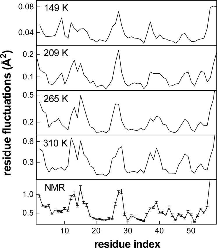
Fluctuations of the Cα atoms, 〈ΔRi · ΔRi〉 well below the dynamic transition (149 K); during the transition (209 K); above the transition (265 K); below unfolding (310 K); and averaged over the 20 NMR structures (Berndt et al., 1992); SE on the mean is shown as bars. Residue-by-residue fluctuation patterns are the same, but note the difference in the absolute value of the fluctuations.
Chain dynamics around the equilibrium state point to the presence of different contributing processes above and below the transition temperature
We characterize the motion of the fluctuation vector by a relaxation function
 |
(2) |
where the overbar denotes the average over all residues and the brackets represent the time average over all time windows of length t in the trajectory. Equation 2 gives the details of the relaxation phenomena in the part of the potential energy surface restricted to the vicinity of the folded structure. The relatively large-scale nature of these motions has contributions from different processes such as harmonic motions between bonded atoms, solvent effects, transitions between conformational substates of the backbone and side chains, as well as larger cooperative fluctuations occurring in, for example, the loop regions.
The overall relaxation is the superposition of many different homogeneous processes with different relaxation times, assuming an exponential decay from all contributing processes. In the sub-ps regime, nonexponential contributions to relaxation phenomena are known to exist (Bizzarri et al., 2000), but such timescales and motions are assumed to be averaged out at the time and length scales explored by the Cα fluctuation dynamics. The collective effect of the relevant dynamical processes, assuming equivalent contribution from each process, is therefore observed as heterogeneous dynamics (Deschenes and Vanden Bout, 2001),
 |
(3) |
where τi is the characteristic timescale of the ith contributing process, and ai is a weighting factor with Σi ai = 1 such that C(0) = 1. Equation 3 may be approximated by the Kohlrausch-Williams-Watts function (Kohlrausch, 1874; Williams and Watts, 1970)
 |
(4) |
Here, τe is a temperature-dependent effective relaxation time representing the average contribution of all the processes affecting the relaxation of the fluctuation vector. The stretch exponent β is 1 for a single process characterized by a simple exponential decay, and it tends to decrease from 1 depending on the number and the timescale of the contributing processes.
Whereas it is evident τe in Eq. 4 is a dynamical parameter, more subtle is the association of β as a thermodynamic quantity (Baysal and Atilgan, 2002). Fluctuations in the thermodynamical entities such as the energy or volume are used to depict phase transitions. Their characterization is achieved by monitoring the relevant susceptibilities such as the heat capacity or isothermal compressibility. Since β was used to describe the protein dynamical transition (Baysal and Atilgan, 2002), we compare its temperature dependence to that of the system heat capacity in Fig. 2, where, at a given temperature, the latter is computed through the relationship, 〈(E − 〈E〉)2〉/kBT2. Both data are represented by two plateau regions with a transition between them in the same temperature range. Best-fitting curves are drawn through the β-data with a Boltzmann sigmoidal function:
 |
(5) |
βo and β1 are the values before and after the transition, λ is a constant governing the slope of the rise during the transition; a similar expression can be written for the heat capacity. λ is 8.0 and 7.4 (7.5), and the transition temperature To is predicted from the inflection point as 193 ± 5 K and 197 ± 4 K (195 ± 4 K) from the heat capacity data and β calculated with 400 ps (200 ps) windows, respectively. Hence, the two curves describe the same type of phenomena, and we can regard β as a type of susceptibility. Conversely, the heat capacity reflects added contributions of individual processes to the energy fluctuations.
FIGURE 2.
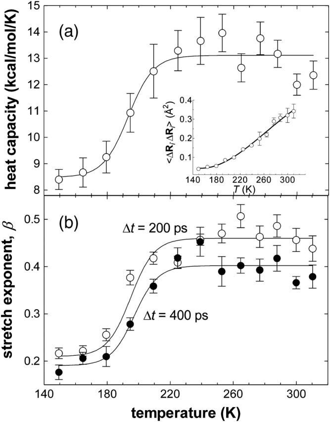
(a) System heat capacity and (b) stretch exponent β, from the fit of Eq. 4 to the relaxation of Cα fluctuations, as a function of temperature. In b, results obtained using two different temporal windows of Δt = 200 and 400 ps are displayed. All curves are best-fit of Boltzmann sigmoidal functions to the data points (Eq. 4). Goodness of fit, determined by the R2 values, is 0.92 in a and 0.94 in b. λ is 8.0 and 7.4 (7.5), and the transition temperature is predicted from the inflection point as 193 ± 5 K and 195 ± 4 (197 ± 4 K) from the heat capacity and β-data with 200 (400) ps temporal windows, respectively. Thermal fluctuations averaged over all residues are also displayed in the inset to (a).
The behavior above is due to the disordered, amorphous character of proteins whereby the stretched exponential decay evidences the complexity of the dynamics involved. It is often argued that this complexity is a result of the superposition of many simple events. As such, it is the details of this dynamics that should reveal the interesting features of protein motions while functioning.
Notice that Fig. 2 b contains the stretch exponent data from the analysis of the trajectories in two separate ways, where the trajectories were partitioned into 200 and 400 ps intervals, respectively. One might argue that this selection will accentuate the contribution of the processes in the selected temporal window. In fact, the data at temperatures below the transition temperature converge to the same values for the two windows, within the uncertainty in the data (0.19 ± 0.02 and 0.21 ± 0.02 for the two respective window sizes). On the contrary, above the transition temperature, two distinct limiting data values are attained (0.40 ± 0.01 and 0.46 ± 0.01 for the two respective window sizes). The origins of these differences will become clear in the next subsection.
Nevertheless, it is demonstrated in Fig. 2 that the dynamical aspects of residue fluctuations involve distinct events below and above the transition, with a gradual (over a temperature range of 50 K) onset of the new events. Thus, the analysis of one variable (residue fluctuations) in two separate ways leads to two seemingly contradictory results: i), equilibrium fluctuations, 〈ΔR2〉, have the same residue-by-residue details (Fig. 1), leading one to assume that the same processes govern at all temperatures despite the presence of a dynamical transition (the latter is also depicted in the inset to Fig. 2 a by the average Cα fluctuations as a function of temperature); and ii), relaxation phenomena, on the other hand, point to the presence of separate processes with different relaxation profiles below and above the dynamical transition (Fig. 2). How is it possible that the dynamical transition that leads to a nonlinear increase in the size of the fluctuations and a functional protein at high temperatures is not manifested in the details of the residue-by-residue fluctuations? And how is it that increasing the temperature and therefore introducing more processes leads to “less complicated” dynamics, implied by the increased value of β (0.4–0.45 above the transition as opposed to 0.2 below)?
A two- versus three-process model provides insight into the nature of the contributing processes to chain dynamics around the equilibrium state
One way to obtain complex relaxation described by the Kohlrausch-Williams-Watts form of Eq. 3 is to include two processes in Eq. 2 with somewhat separate timescales, e.g., two orders of magnitude, 10 and 1000 ps. Let us also consider a third event with an intermediate timescale (e.g., 100 ps). We also assume that each of these processes contribute with a certain weight to the observations. In Fig. 3, we display three superimposed relaxation curves, obtained from Eq. 2, describing the following situations: (i), the two former events, with timescales of 10 and 1000 ps, weighted equally; (ii), all three processes, with timescales of 10, 100, 1000 ps, weighted equally; and (iii), three processes where the fastest two processes contribute twice as much as the slowest process. Also displayed are the curve fits to intermediate times using Eq. 3. Comparing i and ii, we find that the introduction of the transitional event increases β from ∼0.2 to ∼0.4, while decreasing τe; i.e., it leads to a faster relaxation that is relatively closer to a simple exponential. Comparison of ii and iii shows that when the contribution of faster processes are accentuated, the stretch exponent increases to some extent from ∼0.4 to ∼0.45.
FIGURE 3.

Effect of intermediate timescales on the overall dynamics. Assuming there are three processes each showing single exponential decay with relaxation times of 10, 100, and 1000 ps, the cumulative relaxation behaviors are shown with best-fitted stretch exponential curve fits to (i) two processes with τi = 10 and 1000 ps, weighted equally (β = 0.2, τe = 35 ps); (ii) all three processes, weighted equally (β = 0.4, τe = 15 ps); and (iii) all three processes where the fastest two processes contribute twice as much as the slowest process (β = 0.45, τe = 8 ps).
Using the landscape perspective of proteins, we associate the processes governed by the slow timescale (∼1000 ps), with the motion of the overall protein along the envelope of the energy surface defining the folded structure. Processes with the fast timescale (∼10 ps) correspond to the vibrations of the atoms in space, whose more collective manifestation may be monitored through the librational motion of the torsional angles. Their exact form is determined by the pockets decorating the folded-state envelope. Jumps between the pockets are made possible when the molecule gains enough energy, through the heat bath provided by the surrounding medium, to overcome the small energy barriers between them. The frequency of these jumps controls the intermediate regime which becomes accessible once the barriers can be surmounted. The related timescales are intermediate to the other two regimes (∼100 ps).
With this perspective, we may now unify our observations from Figs. 2 b and 3: The long time motions, although slower than our chosen time window in the analysis of the trajectories, will appear in the overall dynamics of the folded protein at all temperatures. They will be reflected onto the dynamics through the slowest modes of motion. Similarly, the fastest motions within the microstates will appear at all temperatures, since these are independent of the jumps between the microstates. The intermediate timescales will only appear when the jumps between the wells are possible. Since our chosen temporal windows of 200 or 400 ps are on the order of this timescale, one would expect the former to accentuate more the fast and intermediate motions compared to the slowest ones, leading to an apparent increase in the stretch exponent. Irrespective of this choice, though, the presence of the intermediate scale is the cause of the phase transition behavior in Fig. 2 b that accompanies the appearance of function in the folded protein, demonstrating that these motions regulate the relevant dynamics.
As regards to the physically meaningful motions that originate the intermediate regime, one must concentrate on those where local collectiveness operates in a way that the protein becomes functional without changing the overall energy landscape of the molecule (due to Fig. 1). Conformational jumps in the torsional angles in the side chains of the surface residues possess both properties; jumps in the backbone torsions, on the other hand, are not good candidates as changes in their rotameric states require the cooperative rearrangement of adjacent dihedral angles and may lead to a population shift toward other parts of the energy landscape.
To corroborate these ideas, we display in Fig. 4 representative torsional angle trajectories of Lys15 which is in the binding loop of BPTI in its complex with β-trypsin. The local fluctuations in the backbone, exemplified by the ψ angle, increase with temperature without a change in the rotameric state. Note that at 310 K, right below the unfolding temperature, attempted rotameric jumps on the backbone are hindered by the landscape, as exemplified by the short-lived jump around 1050 ps. Such changes in the rotameric states of the backbone eventually become accessible on the unfolding pathway that is accessible at higher temperatures (data at 320 K not shown). Side-chain torsional angles, on the other hand, display rotameric jumps at temperatures corresponding to the onset of the dynamical transition, e.g., at 209 K, as shown by the side-chain χ3 angle trajectories in Fig. 4. Note that the librations and jumps are coupled processes, and the former facilitate the faster relaxation of the isomeric jumps by localizing the spatial reorientation of chain segments (Baysal et al., 1996).
FIGURE 4.
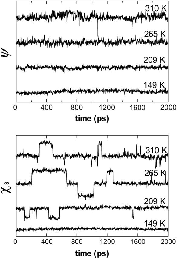
Sample torsional angle trajectories of 2 ns duration for Lys15 at the temperatures of Fig. 2. This residue is in the binding loop of BPTI in its complex with β-trypsin. (Top) Along the backbone, exemplified by the ψ-angle, torsions are constrained so that no conformational jumps between rotational isomeric states are observed; size of the fluctuations, on the other hand, increase above the transition temperature. E.g., average angles and their standard deviations are 78 ± 10° at 149 and 209 K; these become 84 ± 14° and 92 ± 20° at 265 and 310 K, respectively. (Bottom) Along side chains, exemplified by the χ3 angle, torsions are more free to move. In fact, conformational transitions are observed even during the dynamical transition. Well below the transition temperature (149 K), average values are 177 ± 7°; at higher temperatures, the main conformer is still trans with standard deviations of 11, 11, and 15° at 209, 265, and 310 K, respectively.
CONCLUDING REMARKS
The analysis outlined above provides a plain view of the dynamics of a folded protein. The forces holding together the native protein and its hydration shell are strong enough that every detail of the same average structure is maintained regardless of the input of energy from the environment. Thus, although the energy landscape remains unchanged at all temperatures, the system is localized at different regions of the surface at different temperatures, locally experiencing a different part of the energy surface. The onset of short-range cooperative motions at the dynamical transition is associated with the insertion of an intermediate timescale due to the effective sampling of a larger region of the energy surface. We note that these results bear considerable similarity to those derived by Amadei et al. (1999), based on the study of the kinetics in the essential subspace of folded proteins. Therein, the authors pose a physical model whereby the local motions display two diffusion regimes, one on the timescale of a few picoseconds, corresponding to motions within a single harmonic well, and the other on a slower timescale, corresponding to motions between local wells. They also state that the latter are due to the slowest 20 modes of motion, i.e., the collective modes. Our current study, although based on a completely different type of analysis, corroborates these findings and further identifies the origin of the latter diffusive regime in the rotameric jumps between the local states of the side-chain dihedral angles.
We note that our main finding—the functional dynamics is achieved by the insertion of an intermediate timescale between the slowest motions due to the overall relaxation in the broad energy well of the folded protein, and that of the fastest motions due to fluctuations in the microstates—is rooted in an apparent dilemma: Although the size of the fluctuations in the Cα atoms and the relaxation kinetics of the backbone display a clear transition with temperature (Fig. 2 b), the overall residue-by-residue fluctuation pattern of the Cα atoms is independent of temperature in the folded protein (Fig. 1). This latter fact also indicates that different relaxation phenomena are not invoked hierarchically as the temperature increases; rather, the local energy minima communicate in a similar manner at all temperatures, providing similar fluctuation patterns throughout the range studied.
We hypothesize that the same behavior will be observed in all solvents that maintain a similar hydrogen bonding pattern to water (Arcangeli et al., 1998). The transition temperature, however, will be shifted depending on the identity of the bulk solvent (Caliskan et al., 2003). Similarly, dehydrated proteins do not show the dynamical transition, because they do not maintain the right conformations on the protein surface, leading to shifts in the energy landscape. More studies in different solvents and on different proteins should be conducted to clarify these issues.
Proteins perform an organized set of molecular motions such that the loop regions will sample a restricted set of conformations, including those essential for biological activity. The motility gained along the proper landscape, guaranteed by the protein-solvent system, with the activation of the intermediate regime at relatively elevated temperatures, is necessary for the protein to become functional. Once the function (e.g., binding) is realized, however, there are shifts in the energy landscape that affect the stability of the protein (Baysal and Atilgan, 2001) so as to relieve the strain on the system through the shortest possible path (Atilgan et al., 2004).
Acknowledgments
We thank anonymous reviewers for very useful comments and suggestions.
Partial support from Sabanci University Internal Research Grant A0003-00171 and Bogazici University Research Foundation Project 02R102 are gratefully acknowledged. C.B. acknowledges support by the Turkish Academy of Sciences in the framework of the Young Scientist Award Program (CB/TÜBA-GEBIP/2004-3).
References
- Amadei, A., B. L. de Groot, M.-A. Ceruso, M. Paci, A. Di Nola, andH. J. C. Berendsen. 1999. A kinetic model for the internal motions of proteins: diffusion between multiple harmonic wells. Proteins. 35:283–292. [PubMed] [Google Scholar]
- Andersen, H. C. 1983. RATTLE: a ‘velocity’ version of the shake algorithm for molecular dynamics calculations. J. Comput. Phys. 52:24–34. [Google Scholar]
- Arcangeli, C., A. R. Bizzarri, and S. Cannistraro. 1998. Role of interfacial water in the molecular dynamics simulated dynamical transition of plastocyanin. Chem. Phys. Lett. 291:7–14. [Google Scholar]
- Atilgan, A. R., P. Akan, and C. Baysal. 2004. Small-world communication of residues and significance for protein dynamics. Biophys. J. 86:85–91. [DOI] [PMC free article] [PubMed] [Google Scholar]
- Baysal, C., and A. R. Atilgan. 2001. Coordination topology and stability for the native and binding conformers of chymotrypsin inhibitor 2. Proteins. 45:62–70. [DOI] [PubMed] [Google Scholar]
- Baysal, C., and A. R. Atilgan. 2002. Relaxation kinetics and the glassiness of proteins: the case of bovine pancreatic trypsin inhibitor. Biophys. J. 83:699–705. [DOI] [PMC free article] [PubMed] [Google Scholar]
- Baysal, C., A. R. Atilgan, B. Erman, and I. Bahar. 1996. Molecular dynamics analysis of coupling between librational motions and isomeric jumps in chain molecules. Macromolecules. 29:2510–2514. [Google Scholar]
- Berman, H. M., J. Westbrook, Z. Feng, G. Gilliland, T. N. Bhat, H. Weissig, I. N. Shindyalov, and P. E. Bourne. 2000. The protein data bank. Nucleic. Acids Res. 28:235–242. [DOI] [PMC free article] [PubMed] [Google Scholar]
- Berndt, K. D., P. Guntert, L. P. M. Orbons, and K. Wuthrich. 1992. Determination of a high-quality nuclear magnetic resonance solution structure of the bovine pancreatic trypsin inhibitor and comparison with three crystal structures. J. Mol. Biol. 227:757–775. [DOI] [PubMed] [Google Scholar]
- Bizzarri, A. R., A. Paciaroni, and S. Cannistraro. 2000. Glasslike dynamical behavior of the plastocyanin hydration water. Phys. Rev. E. 62:3991–3999. [DOI] [PubMed] [Google Scholar]
- Caliskan, G., A. Kisliuk, A. M. Tsai, C. L. Soles, and A. P. Sokolov. 2003. Protein dynamics in viscous solvents. J. Chem. Phys. 118:4230–4236. [Google Scholar]
- Daniel, R. M., J. C. Smith, M. Ferrand, S. Hery, R. Dunn, and J. L. Finney. 1998. Enzyme activity below the dynamical transition at 220 K. Biophys. J. 75:2504–2507. [DOI] [PMC free article] [PubMed] [Google Scholar]
- Dastidar, S. G., and C. Mukhopadhyay. 2003. Structure, dynamics, and energetics of water at the surface of a small globular protein: a molecular dynamics simulation. Phys. Rev. E. 68:021921-1–021921-9. [DOI] [PubMed] [Google Scholar]
- Dauber-Osguthorpe, P., V. A. Roberts, D. J. Osguthorpe, J. Wolff, M. Genest, and A. T. Hagler. 1988. Structure and energetics of ligand binding to proteins: E. coli dihydrofolate reductase-trimethoprim, a drug-receptor system. Proteins. 4:31–47. [DOI] [PubMed] [Google Scholar]
- Deschenes, L. A., and D. A. Vanden Bout. 2001. Single-molecule studies of heterogeneous dynamics in polymer melts near the glass transition. Science. 292:255–258. [DOI] [PubMed] [Google Scholar]
- Dvorsky, R., J. Sevcik, L. S. D. Caves, R. E. Hubbard, and C. S. Verma. 2000. Temperature effects on protein motions: a molecular dynamics study of RNase-Sa. J. Phys. Chem. 104:10387–10397. [Google Scholar]
- Fenimore, P. W., H. Frauenfelder, B. H. McMahon, and F. G. Parak. 2002. Slaving: solvent fluctuations dominate protein dynamics and functions. Proc. Natl. Acad. Sci. USA. 99:16047–16051. [DOI] [PMC free article] [PubMed] [Google Scholar]
- Garcia, A. E., R. Blumenfeld, G. Hummer, and J. A. Krumhansl. 1997. Multi-basin dynamics of a protein in a crystal environment. Physica D. 107:225–239. [Google Scholar]
- Garcia, A. E., and G. Hummer. 1999. Conformational dynamics of cytochrome c: correlation to hydrogen exchange. Proteins. 36:175–191. [PubMed] [Google Scholar]
- Halle, B. 2004. Biomolecular cryocrystallography: structural changes during flash-cooling. Proc. Natl. Acad. Sci.USA. 101:4793–4798. [DOI] [PMC free article] [PubMed] [Google Scholar]
- Hayward, J. A., and J. C. Smith. 2002. Temperature dependence of protein dynamics: computer simulation analysis of neutron scattering properties. Biophys. J. 82:1216–1225. [DOI] [PMC free article] [PubMed] [Google Scholar]
- Kohlrausch, R. 1874. Theorie des elektrischen Rückstandes in der Leidener Flasche. Ann. Phys. Chem. (Leipzig). 91:179–214. [Google Scholar]
- Kriminski, S., M. Kazmierczak, and R. E. Thorne. 2003. Heat transfer from protein crystals: implications for flash cooling and x-ray beam heating. Acta Crystallogr. D. 59:697–708. [DOI] [PubMed] [Google Scholar]
- Miyazaki, Y., T. Matsuo, and H. Suga. 2000. Low-temperature heat capacity and glassy behavior of lysozyme crystal. J. Phys. Chem. B. 104:8044–8052. [Google Scholar]
- Nose, S. 1984. A molecular dynamics method for simulations in the canonical ensemble. Mol. Phys. 50:255–268. [Google Scholar]
- Pal, S. K., J. Peon, and A. H. Zewail. 2002. Biological water at the protein surface: dynamical solvation probed directly with femtosecond resolution. Proc. Natl. Acad. Sci. USA. 99:1763–1768. [DOI] [PMC free article] [PubMed] [Google Scholar]
- Tarek, M., and D. J. Tobias. 2002. Role of protein-water hydrogen bond dynamics in the protein dynamical transition. Phys. Rev. Lett. 88:138101-1–138101-4. [DOI] [PubMed] [Google Scholar]
- Tournier, A. L., J. Xu, and J. C. Smith. 2003. Translational hydration water dynamics drives the protein glass transition. Biophys. J. 85:1871–1875. [DOI] [PMC free article] [PubMed] [Google Scholar]
- Tsai, A. M., T. J. Udovic, and D. A. Neumann. 2001. The Inverse relationship between protein dynamics and thermal stability. Biophys. J. 81:2339–2343. [DOI] [PMC free article] [PubMed] [Google Scholar]
- Vitkup, D., D. Ringe, G. A. Petsko, and M. Karplus. 2000. Solvent mobility and the protein ‘glass’ transition. Nat. Struct. Biol. 7:34–38. [DOI] [PubMed] [Google Scholar]
- Williams, G., and D. C. Watts. 1970. Non-symmetrical dielectric relaxation behavior arising from a simple empirical decay function. Trans. Faraday Soc. 66:80–85. [Google Scholar]
- Wlodawer, A., J. Walter, L. Huber, and L. Sjolin. 1984. Structure of bovine pancreatic trypsin inhibitor. Results of joint neutron and x-ray refinement of crystal form II. J. Mol. Biol. 180:301–329. [DOI] [PubMed] [Google Scholar]
- Zaccai, G. 2000. How soft is a protein? A protein dynamics force constant measured by neutron scattering. Science. 288:1604–1607. [DOI] [PubMed] [Google Scholar]
- Zaccai, G. 2003. Proteins as nano-machines: dynamics-function relations studied by neutron scattering. J. Phys. Condens. Matter. 15:S1673–S1682. [Google Scholar]