Intrinsic and extrinsic contributions to stochasticity in gene expression

Abstract

Gene expression is a stochastic, or “noisy,” process. This noise comes about in two ways. The inherent stochasticity of biochemical processes such as transcription and translation generates “intrinsic” noise. In addition, fluctuations in the amounts or states of other cellular components lead indirectly to variation in the expression of a particular gene and thus represent “extrinsic” noise. Here, we show how the total variation in the level of expression of a given gene can be decomposed into its intrinsic and extrinsic components. We demonstrate theoretically that simultaneous measurement of two identical genes per cell enables discrimination of these two types of noise. Analytic expressions for intrinsic noise are given for a model that involves all the major steps in transcription and translation. These expressions give the sensitivity to various parameters, quantify the deviation from Poisson statistics, and provide a way of fitting experiment. Transcription dominates the intrinsic noise when the average number of proteins made per mRNA transcript is greater than ≃2. Below this number, translational effects also become important. Gene replication and cell division, included in the model, cause protein numbers to tend to a limit cycle. We calculate a general form for the extrinsic noise and illustrate it with the particular case of a single fluctuating extrinsic variable—a repressor protein, which acts on the gene of interest. All results are confirmed by stochastic simulation using plausible parameters for Escherichia coli.

Molecules are discrete entities. When present in large numbers, addition or removal of any single molecule typically has little effect on the properties of a system. However, stochastic fluctuations can become significant in smaller systems. In living cells, many components are present at very low copy numbers, [e.g., of order one for DNA loci and of order tens for transcription factors (1)]. Therefore, stochastic effects are thought to be particularly important for gene expression and have been invoked to explain cell–cell variations in clonal populations (2–4). Indeed, cellular components interact with one another in complex regulatory networks. Thus, fluctuations in even a single component may potentially affect the performance of the entire system.

Consider a particular gene of interest. The amount of protein it produces will vary from cell to cell in a population and over time in a single cell. These fluctuations originate in two ways: First, even if all cells were in precisely the same state, the reaction events leading to transcription and translation of the gene would still occur at different times, and in different orders, in different cells. Such stochastic effects are set locally by the gene sequence and the properties of the protein it encodes and will be referred to as “intrinsic” noise.

In addition, one must consider that other molecular species in the cell, e.g., RNA polymerase (RNAP), are themselves gene products and therefore will also vary over time and from cell to cell. This variation causes additional, and corresponding, fluctuations in the expression of the gene of interest that will be referred to as “extrinsic” noise. Thus, extrinsic sources of noise arise independently of the gene but act on it. Examples of extrinsic variables are numerous. They include the number of RNAPs or ribosomes, the stage in the cell cycle, the quantity of the protein, and mRNA degradation machinery, and the cell environment. In general, the total variation in gene expression will have both intrinsic and extrinsic sources. A particular cellular component will suffer intrinsic fluctuations in its own concentration and, at the same time, will be a source of extrinsic noise for other components with which it interacts.

Although the stochastic nature of gene expression has long been postulated (2), previous theoretical research (5–11) has concentrated on intrinsic noise. Excepting studies of plasmid copy number control (12), extrinsic effects have only been added in a post hoc manner (13). It is not known which molecular properties influence noise or even how a clear measurement of intrinsic noise could be obtained in vivo.

This paper seeks to address several problems. First, we distinguish between intrinsic and extrinsic sources of noise and integrate both within a single framework. Second, we model intrinsic noise at a level that allows direct connection with biochemical parameters, including those related to cell growth. Third, we suggest an experimental method that can be used to discriminate and quantify the two components of noise in living cells. Our approach, by integration of intrinsic and extrinsic effects, is general enough to allow comparison with experimental data (14).

Definitions

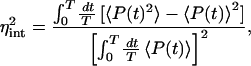
Fluctuations in the rates of transcription and translation of a particular gene result in corresponding fluctuations in the amount of its protein product. A natural and biologically relevant measure of the magnitude of gene expression noise is thus the size of protein fluctuations compared to their mean concentration. If P(t) is the protein concentration at time t, then the protein noise, η(t), is given by

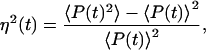1

where the angled brackets denote an average over the probability distribution of P at time t. We will similarly use standard deviation divided by mean, or coefficient of variation, as a measure of noise in other distributions.

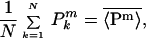
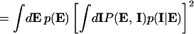
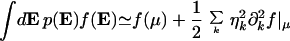
To examine the noise for a particular gene across a cell population, let the intrinsic and extrinsic variables (including time—cells are typically desynchronized) for that gene be given by vectors I and E, each of whose components represent a different source of noise. The expression level of the gene in one cell, as measured experimentally, is denoted P_k (with k a cell label). From a snapshot of N genetically identical cells, the P_ks can be averaged to find the moments of the protein distribution. This averaging process (where m = 1 and m = 2 for the mean and variance, respectively) is equivalent to

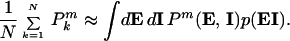2

Here p(EI) is the probability density function for the intrinsic and extrinsic variables, and P(E, I) is the measured expression level for particular values of E and I. Using the product rule of probabilities, this becomes

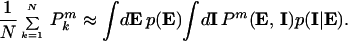3

The second integral is an average over the intrinsic variables with the extrinsic variables held fixed and shall be denoted by angled brackets:

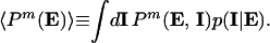4

Averages over the extrinsic variables will be indicated with an overbar, so that Eq. 3 becomes

5

that is, an average over both intrinsic and extrinsic noise sources.

Hence, the measured noise, η_tot, defined empirically by

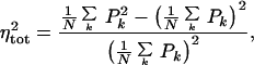6

is equivalent to

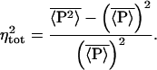7

This can be written as

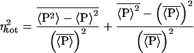8

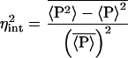
In other words, the square of the experimentally measurable noise is a direct sum of the intrinsic, η_int, and extrinsic, η_ext, contributions. The intrinsic noise, η_int, is proportional to the variance of the intrinsic distribution, calculated for a particular value of the extrinsic variables and then averaged over all possible values of these variables. The extrinsic noise, η_ext, vanishes as the extrinsic distributions become more and more spiked.

Finally, we need to address experimentally how both intrinsic and extrinsic contributions can be discriminated from the total noise, given by Eq. 6. From Eq. 8, this requires a measurement of the quantity . Consider what would happen if two identical copies of the gene were present in the same (kth) cell, and their protein products, labeled P and P, were measured simultaneously. These will have different values of the intrinsic variables, but, because both are present in a single cell, they will be exposed to the same intracellular environment and so have the same value of the extrinsic variables. Therefore, by summing their product, we obtain

9

precisely the average needed.

Experimentally, two distinguishable variants of green fluorescent protein, corresponding to P⁽¹⁾ and P⁽²⁾, would allow estimation of Eq. 9 (14). By considering quantities such as ∑_k(P − P)², the intrinsic noise could be measured and η_ext extracted from the total noise by using Eq. 8.

Expressions for Intrinsic Noise

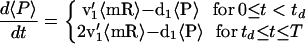
To understand the sources of intrinsic fluctuations, consider the simplified model of gene expression shown in Fig. 1. All extrinsic variables (excepting time) are set to constant values; thus, the binding of RNAP, ribosomes, and degradosomes, for example, become first-order processes as their respective concentrations are held fixed. We model the bacterial cell cycle by allowing the gene copy number, n, to double at some (fixed) time t_d into each cycle and to halve at cell division (time T). Non-DNA molecular species are randomly distributed at cell division between the two daughter cells.

Figure 1.

Reaction scheme detailing constitutive expression of a protein P. All molecular species shown are intrinsic variables. Transcription is modeled (15) as reversible binding of RNAP to promoter, D (rates f₀ and b₀). Isomerization from closed to open complex and initiation of transcription are approximated as a first-order process (rate k₀). Only the leader region of the mRNA, mR^U, is followed. It is made by transcribing polymerase, T, at rate ν₀. mRNA is degraded by the binding of the degradosome (rate mf₀) to form complex mC¹, which decays in a first-order manner. Following ref. 6, ribosomes compete with degradosomes for the leader region of the mRNA and bind reversibly (rates mf₁ and mb₁). Start of translation is from the mC² state with rate k₁, which frees mR^U for further binding. Protein is translated (rate ν₁) in the mT state and decays with rate d₁. Inset shows a simplified model of translation, with mR now designating an entire mRNA molecule, degrading at rate d′₀, and is translated with rate ν′₁.

Fig. 1 Inset shows a simplified version of the model that can be solved analytically. Two effective rate constants, marked with primes, have been introduced and can be related to those of the full system. The mRNA half-life is given by the set of differential equations describing 〈mR^U〉 and 〈mC²〉: d′₀ ≃ log 2 × (ℓ₁ − ℓ₀)/2 with ℓ₁ = k₁ + mb₁ + mf₀ + mf₁ and ℓ = ℓ − 4 mf₀(k₁ + mb₁). The number of proteins made from a particular mRNA is distributed geometrically (similar to ref. 6), and so the mean number of proteins produced per transcript, b, can be shown to be

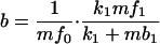10

and the overall translation rate is ν′₁ = bd′₀, by definition.

Simulation Results

Stochastic simulation (16, 17) was used to model the scheme of Fig. 1 by using parameter values published as supporting information on the PNAS web site, www.pnas.org. The probability of a given reaction occurring is equal to the product of the rate constant for that reaction and the number of potential reactants present. Time steps between reactions obey a Markov process and take account, for binary reactions, of the growing cell volume (17). The latter increases linearly (18) from an initial value until cell division (at time T), when it halves. Gene doubling and binomial partitioning of non-DNA molecules are included, and one daughter cell is followed at each division.

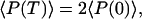
After a sufficient number of divisions, the protein number and concentration tend not to a steady-state but rather to the limit cycle (whose period is set by cell division), shown in Fig. 2. The slight kink in the protein number curve is due to the increased rate of protein production as the number of genes doubles (chosen arbitrarily to be at time t_d = 0.4T into the cell cycle). The protein concentration is approximately the same before and after cell division once the limit cycle state has been reached. It falls initially (before gene replication) as protein is produced at a rate slower than that of cell growth.

Figure 2.

Simulation results for protein and mRNA number using the model of Fig. 1 Inset. A strong promoter is used (k₀ = 0.1 s⁻¹), and there is just one copy of the gene on the chromosome. On average, 15 proteins are synthesized per mRNA transcript, and the mRNA half-life is 1 min. Gene replication occurs every t_d = 0.4T into the cell cycle and is marked with a small dot on the time axis. All other parameters are given in the supporting information. The total noise η_tot is defined in Eqs. 6 and 7, with the overbar, in this simple case, just denoting a time (cell cycle) average. This is given for each species in the upper right-hand corner.

The time scales associated with transcription and mRNA degradation are much shorter than the protein decay rate or the cell cycle time (see supporting information). Therefore, mRNA levels alternate between two approximately steady states, with a short transient in between. Despite the noise, this effect can be discerned in Fig. 2 (compare numbers for t < t_d with those for t > t_d).

Analytical Results

Assuming that the molecules involved in transcription are in one of two steady states (depending on the gene copy number n), and that all other time dependence is absorbed into the protein distribution, then the simpler model, shown in Fig. 1 Inset, can be substituted for the full scheme and solved analytically (see supporting information).

The mean mRNA number satisfies

11

before replication, t < t_d and twice this result for t > t_d. Here, ℓ = f₀ + b₀ + k₀.

The mean protein number, which changes with time, obeys

12

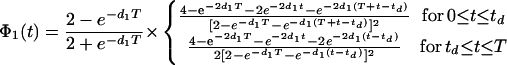
with φ₀ a continuous function of t,

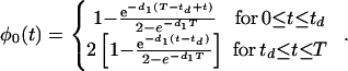13

Note that the factor of two arising from gene replication is absorbed into the function φ₀, and so 〈mR〉 in Eq. 12 is given by Eq. 11 regardless of t being greater or less than t_d.

Eqs. 12 and 13 can be understood as being the solution of

14

with continuity at t = t_d and the limit cycle boundary condition

15

which arises because of the partition at each cell division (see Fig. 2 Upper), that is, a simple birth-and-death process with the birth rate doubling after gene replication.

The noise in mRNA number is

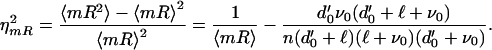16

Eq. 16 is less than the Poisson value, 1/〈mR〉, because conservation of DNA species limits the maximum amount of C that can be present. This in turn gives an upper bound to the rate at which T is created, narrowing the distribution of T. A narrower T distribution leads to a narrower mRNA distribution and so to the negative term in Eq. 16. Typically, however, this correction is rarely large.

The intrinsic noise in protein number (denoted η̂_int, rather than η_int, as the extrinsic variables have not yet been averaged away) satisfies in the limit small d₁/d′₀ (see supporting information for the full expression),

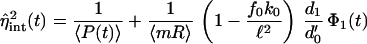17

with

18

for each traversal of the limit cycle. Note that 1/〈P〉 is also of order d₁/d′₀ from Eq. 12 as ν′₁ = bd′₀. Eq. 17 contains a Poisson term, the mean 〈P(t)〉, and a non-Poisson term, which is a measure of the stochastic effects present in transcription. The limit d₁/d′₀ ≪ 1 taken is expected to be valid for many genes in E. coli, because protein lifetimes are typically hours, whereas those of mRNA are only minutes (see supporting information).

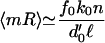
Fig. 3 shows the good agreement between theory and simulation. Because of the difference in gene copy number, the number of mRNAs for t > t_d is approximately twice that for t < t_d (see Eq. 11). If cell cycle effects are temporarily set aside, the protein noise, dominated by mRNA number, will therefore be higher for a gene copy number of n than for a gene copy number of 2n. However, because of the cell cycle, immediately after cell division the protein noise is low (being still determined by the previous 2n gene state) and will grow for 0 < t < t_d as it tends toward the higher value set by the cell being in a n gene state. Immediately after gene replication, the noise is high (from the cell having just left the n gene regime) and so for t_d < t < T will fall as it tends toward the lower value prescribed by the cell's 2n state. Consequently, the intrinsic protein noise goes through a maximum at t = t_d.

Figure 3.

Comparison of analytic solution and stochastic simulation. The noise in protein level (averaged over 5,000 runs) for the three different models is plotted as a function of time (in units of the cell cycle). Upper light dotted curve is the result of a simulation of the full model of protein expression, Fig. 1, with k₀ = 0.01 s⁻¹. Dotted curve is a simulation of Fig. 1 Inset, whereas the full curve is a plot of Eq. 17. At the beginning of the cell cycle, η̂_int is slightly greater than that at the end because of the random partitioning of proteins and mRNA into daughter cells on division.

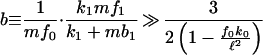
The intrinsic noise, via Eq. 12 and using ν′₁ = bd′₀, can also be written as

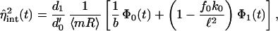19

with Φ₀(t) = 1/φ₀(t) given in Eq. 13. The parameter dependence and form of Eq. 19 can in fact be shown to hold for the full model of Fig. 1 when d₁/d′₀ ≪ 1. By inspecting Eq. 19, only the first term depends on the parameters controlling translation rates. Therefore, if the second term dominates the first, transcription rather than translation will determine protein intrinsic noise. Expanding in d₁T, this condition is fulfilled if

20

for d₁T ≪ 1. As 1 − f₀k₀/ℓ² ≥ 3/4, Eq. 20 will certainly be satisfied, and so transcription will dominate over translation if the number of proteins per transcript (or burst size in the terminology of refs. 6 and 10) is much greater than two, i.e., b ≫ 2. In fact, the number of proteins per transcript may be of order tens (19) (although individual translation rates vary widely). In such cases, we conclude that transcription is the chief source of intrinsic noise. From Eq. 20, noise at translation becomes important only if mf₁, the rate of ribosome binding, and k₁, the rate of commitment of a bound ribosome to carrying out translation, are low and if mf₀, the rate of mRNA degradation, is high.

Previous work claimed that translation controls protein noise (10). This conclusion was reached by using an alternative noise definition (variance, rather than standard deviation, over the mean), which divides out all dependence on transcriptional parameters. In contrast, Eq. 19 treats transcription and translation on an equal footing and keeps all parameter dependence explicit. (For example, if the gene copy number, n, is increased 100-fold, the noise is reduced as expected intuitively.) The conclusion that translation is a minor contributor to noise (for b > 2) is thus transparent. This conclusion is also confirmed by recent independent simulations of LacZ expression (7).

Eq. 19 makes explicit the dependence of the intrinsic noise on the parameters shown in Fig. 1. A high ratio of protein to mRNA lifetime (low d₁/d′₀) reduces noise. Given Eq. 11, the importance of the rates controlling the initiation of transcription can be seen; both terms in Eq. 19 decrease for high f₀, the “on” rate of the RNAP, a large isomerization rate, k₀, and to a lesser extent a low RNAP “off” rate, b₀. The square of the noise is independent of ν₀ and ν₁ and varies inversely with the gene copy number, n. Thus, for example, fast-growing bacteria, which undergo multiple rounds of initiation of DNA replication before division, are therefore expected to be intrinsically less noisy because of their higher n values (depending on gene distance from the origin of replication). The additional parameter dependence when translation also becomes important, i.e., when b ≪ 2 and η² ∼ 1/b, is given by Eq. 10.

To illustrate the role of the cell cycle and the significance of the gene replication time, t_d, let us, for the moment, ignore all other effects and assume that time is the only extrinsic variable. Then, the extrinsic average (the overbar) in Eq. 8 is just a cell cycle average and

21

for example. This experimentally accessible value is an approximation to the “true” average value of the intrinsic noise, ∫ dt η̂ (t), which involves only one integral and not two. Table 1 demonstrates the validity of Eq. 21 as an estimate of the true noise and the excellent agreement between theory and simulation.

Table 1.

Comparison of theory and simulation for a constitutively expressed gene

η	Protein nos.		Protein concentration
	Simulation	Theory	Simulation	Theory
ηtot	0.26  ± 0.003	0.26	0.15  ± 0.005	0.15
ηint	0.15  ± 0.007	0.15	0.15  + 0.007	0.15
ηext	0.21  ± 0.004	0.21	0.05  ± 0.01	0.04

Time is the only extrinsic value, and there is consequently almost no extrinsic noise in the protein concentration (because this varies little during the cell cycle; see Fig. 2). The intrinsic noise in both cases, calculated by Eq. 21 (with an appropriate expression for cell volume when needed), is a very good approximation to ∫dtη̂, which is found to be 0.15 ± 0.008 from simulation and 0.15 from integrating Eq. 17. Parameter values are published as supporting information on the PNAS web site, except k₀ = 0.01 s⁻¹. Values stated are mean results from 100 simulations and errors are ±1 SD. 

In the limit where d₁T → 0 (appropriate for GFP in E. coli), protein does not decay but is diluted only because of partition at each cell division. Eq. 21 is then simple to evaluate and satisfies (with τ_d = t_d/T)

22

Both terms in Eq. 22 can be seen to increase monotonically with τ_d = t_d/T; a low t_d implies that the cell spends most time in the high gene copy number state, 2n, and so protein and mRNA levels increase, reducing noise. As t_d/T increases, Eq. 22 varies by a factor of around 0.35 to 0.7. Thus, a steady-state approximation, in which time dependence is ignored (Φ₀ = Φ₁ = 1), could overestimate intrinsic noise by as much as 65%.

Expressions for Extrinsic Noise

Time is, of course, not the only extrinsic variable; the sources of extrinsic noise are multiple, ranging from fluctuations in the bacterial growth rate to changes in the degree of DNA supercoiling and are often poorly understood. The simplest way to model these effects is to let each extrinsic variable, E_k, have mean μ_k and standard deviation, σ_k, and an independent, normal distribution. Using asymptotic expansion methods (20), performing an extrinsic average of a function f(E) then gives

23

in the limit of small extrinsic noise, η_k = σ_k/μ_k. Here we write ∂_k for a partial derivative with respect to the variable x_k = E_k/μ_k.

The extrinsic average arises in Eq. 8 as, experimentally, averages are taken over a population of cells, each cell having a different set of values of the extrinsic variables. The theoretical intrinsic noise, Eq. 19, is calculated with all extrinsic variables fixed and therefore needs a correction term before it can be properly compared with experiment. Rather than also average over time explicitly, we will, for the sake of clarity, treat it just as a parameter in this section. The intrinsic noise, η, then satisfies, via Eq. 23,

24

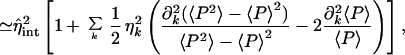with η̂_int given by Eq. 17 and all the extrinsic variables set to their mean values, μ_k. Experimentally, it is possible to continuously vary the rate of transcription from certain inducible promoters (14, 21). Eq. 24 implies that there is a correction to the more naive expectation, from Eq. 19, that the intrinsic noise should vary as the inverse square of induction level (assuming that the latter is proportional to the number of mRNAs).

The extrinsic noise, η_ext, obeys

25

with all extrinsic variables set to their mean and χ_k = (∂_k log〈P〉)² defined, in analogy with statistical physics, as a noise “susceptibility.” The individual χ_k measure the contribution of a particular extrinsic process to the total noise strength.

An Example: Repression

To illustrate the effects of a fluctuating extrinsic variable, we consider a gene of interest that is repressed by another extrinsic protein. The repressor has a noise given by Eq. 17 with the appropriate parameter values for its own expression. To find the intrinsic noise, from Eq. 9, we assume that two identical copies of our gene are present, both acted on by the same repressor.

Repression is modeled by the repressor, R, binding to the promoter and preventing access to it by RNAP (ref. 22). This repressor–DNA complex forms and decomposes with rates f₁ and b₁, respectively, implying that the mean mRNA number of the (repressed) protein obeys

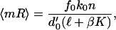26

where β = b₀ + k₀ and K = f₁/b₁.

In Eq. 26, to make the extrinsic repressor concentration explicit, the “on” rate (which is really a second-order process) should be written as f₁ = f̂₁μ_rep, where f̂₁ is the binding rate of a single repressor to DNA, and μ_rep, the mean repressor number. Applying the definition of χ_k to Eq. 12, with 〈mR〉 given by Eq. 26, the repressor noise susceptibility can be found, and Eq. 8 becomes

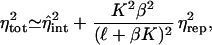27

where η̂ is given by

28

with Eq. 26 again.

The total, intrinsic, and extrinsic noises found by simulation are compared with the corresponding theoretical values (with time again included properly as an extrinsic variable) in Table 2. The good agreement, as well as validating Eqs. 27 and 28, also demonstrates the suitability of the Gaussian approximation implicit in Eq. 23 as the repressor is expressed in the simulation using the full scheme of Fig. 1 and not added in an ad hoc manner.

Table 2.

Comparison of theory and simulation for a gene acted on by a repressor

η	Simulation	Theory
ηtot	0.51  ± 0.02	0.51
ηint	0.45  ± 0.02	0.44
ηext	0.24  ± 0.03	0.26

There are two extrinsic variables: time and the repressor. Noise is calculated for protein numbers, not concentrations. To find the intrinsic noise, two copies of the (repressed) gene were simulated (see text). All proteins (including the repressor) were created according to the full scheme of Fig. 1 (with, for simplicity, the same rate constants, although different t_ds). Parameter values are given in the supporting information, except k₀ = 0.01 s⁻¹, f̂₁ = 5 × 10⁷M⁻¹⋅s⁻¹, b₁ = 0.33 s⁻¹, and t_d = 0.7T for the repressor gene. η_rep is calculated to be 0.17 by integrating Eq. 17 over one cell cycle. Because of the repressor, expression is reduced to about 10% of its constitutive level (the expression level of Table 1). Values given are mean results from 100 simulations, and errors are ±1 SD. 

The repressor noise may dominate the extrinsic noise to such an extent that Eq. 27 is still valid when all other extrinsic variables fluctuate. For example, in ref. 14, the transcription rate of two distinguishable alleles of gfp, both having the same regulatory sequences, is controlled by a repressor. When the repressor concentration is systematically varied from low to high values (by adding different amounts of inducer), the extrinsic noise goes through a maximum (14). This phenomenon can be understood by realizing that the extrinsic noise is dominated by the repressor. Although χ_rep increases with increasing repressor concentration, η_rep, the noise in repressor number, decreases. As a result of these two opposing behaviors, η_ext (and therefore η_tot) exhibits a maximum as a function of repressor concentration. This behavior illustrates clearly the importance of noise susceptibilities in setting cell–cell variation.

Conclusion

We have presented a theoretical framework that enables interpretation of experimental measurements of stochasticity in gene expression. Cell–cell variation in expression of a single gene (η_tot) is not a direct measure of intrinsic noise. Rather, it contains both intrinsic and extrinsic contributions. In particular, extrinsic noise, a consequence of the different local environments of the gene in the different cells, must be considered.

Only the intrinsic variables (given in Fig. 1) vary from gene to gene, as well as moment to moment, within a particular cell. By changing the parameters that influence these variables, the cell can locally affect the noise in expression of a given gene. On the other hand, alterations in the extrinsic variables can potentially affect all genes within the cell (although the magnitude of these effects for one gene may be very different from those for another). Eqs. 17 and 19 are analytical expressions for the major component of the intrinsic noise. There is a Poisson term, expected for a birth-and-death process, determined by the protein mean, and an additional contribution coming from the noise generated during transcription (essentially a time average of the noise in mRNA level). Two noise regimes exist: if the translation efficiency, or burst size (6), b, is high (more than two proteins per transcript), as is believed to be typical in E. coli, then transcription dominates intrinsic noise. Otherwise, translational effects must also be considered.

All the major steps in transcription and translation are accounted for, and the complete parameter dependence of the noise is given by Eq. 19 with Eq. 10. Intrinsic noise (except possibly for very short lived proteins) is unaffected by ν₀ and ν₁, the rates of transcription by RNAP and translation by a ribosome, respectively. As transcription usually dominates, f₀ and b₀, the “on” and “off” rates of RNAP as well as the isomerization rate, k₀, strongly influence noise. Longer-lived proteins (compared to mRNA lifetimes) and genes with high copy number are less stochastic. The chromosomal position of the gene also controls intrinsic noise—genes replicated early being less noisy.

The cell cycle drives protein numbers and intrinsic noise to a limit cycle. Protein numbers can be significantly different from the steady-state approximations used in the literature. The intrinsic noise itself does not change appreciably during the course of the cell cycle, but the cell cycle is crucial in determining its absolute magnitude.

The extrinsic noise is expected to be a linear sum of the noise in each of the extrinsic variables (see Eq. 25), where the coefficients play the role of noise “susceptibilities.” These susceptibilities determine the relative importance of each term in the total extrinsic noise and allow exploration of how the environment in which a gene is expressed influences its expression level. By simulating a repressed gene, where the repressor number is the only fluctuating extrinsic variable, we have verified our analytical expressions are quantitatively correct. Experimentally, the intrinsic and extrinsic noise can often be of similar magnitude (14). For a given gene, however, the quantity of interest is usually the intrinsic noise, which we have shown here can be measured by monitoring expression from two identical copies of the same gene integrated into each cell (see also ref. 14).

Our theoretical framework should provide support for experimental research (14) aimed at discovering whether noise is detrimental to the cell, whether it can be “regulated away” with higher-level circuitry (23), and to what extent it might confer evolutionary advantages on a clonal population.

Abbreviation

RNAP

RNA polymerase

References

- 1.Guptasarma P. BioEssays. 1995;17:987–997. doi: 10.1002/bies.950171112. [DOI] [PubMed] [Google Scholar]
- 2.Spudich J L, Koshland D E., Jr Nature (London) 1976;262:467–471. doi: 10.1038/262467a0. [DOI] [PubMed] [Google Scholar]
- 3.McAdams H H, Arkin A. Trends Genet. 1999;15:65–69. doi: 10.1016/s0168-9525(98)01659-x. [DOI] [PubMed] [Google Scholar]
- 4.Arkin A, Ross J, McAdams H H. Genetics. 1998;149:1633–1648. doi: 10.1093/genetics/149.4.1633. [DOI] [PMC free article] [PubMed] [Google Scholar]
- 5.Ko M S H. J Theor Biol. 1991;153:181–194. doi: 10.1016/s0022-5193(05)80421-7. [DOI] [PubMed] [Google Scholar]
- 6.McAdams H H, Arkin A. Proc Natl Acad Sci USA. 1997;94:814–819. doi: 10.1073/pnas.94.3.814. [DOI] [PMC free article] [PubMed] [Google Scholar]
- 7.Kierzek A M, Zaim J, Zielenkiewicz P. J Biol Chem. 2001;276:8165–8172. doi: 10.1074/jbc.M006264200. [DOI] [PubMed] [Google Scholar]
- 8.Berg O G. J Theor Biol. 1978;71:587–603. doi: 10.1016/0022-5193(78)90326-0. [DOI] [PubMed] [Google Scholar]
- 9.Peccoud J, Ycart B. Theor Popul Biol. 1995;48:222–234. [Google Scholar]
- 10.Thattai M, Van Oudenaarden A. Proc Natl Acad Sci USA. 2001;98:8614–8619. doi: 10.1073/pnas.151588598. [DOI] [PMC free article] [PubMed] [Google Scholar]
- 11.Kepler T B, Elston T C. Biophys J. 2001;81:3116–3136. doi: 10.1016/S0006-3495(01)75949-8. [DOI] [PMC free article] [PubMed] [Google Scholar]
- 12.Paulsson J, Ehrenberg M. Q Rev Biophys. 2001;34:1–59. doi: 10.1017/s0033583501003663. [DOI] [PubMed] [Google Scholar]
- 13.Hasty J, Pradines J, Dolnik M, Collins J J. Proc Natl Acad Sci USA. 2000;97:2075–2080. doi: 10.1073/pnas.040411297. [DOI] [PMC free article] [PubMed] [Google Scholar]
- 14.Elowitz M B, Levine A J, Siggia E D, Swain P S. Science. 2002;297:1183–1186. doi: 10.1126/science.1070919. [DOI] [PubMed] [Google Scholar]
- 15.Record T M, Reznikoff W S, Craig M L, McQuade K L, Schlax P J. In: Escherichia coli and Salmonella: Cellular and Molecular Biology. Neidhardt F C, editor. Washington, DC: Am. Soc. Microbiol.; 1996. pp. 792–821. [Google Scholar]
- 16.Gillespie D T. J Phys Chem. 1977;81:2340–2361. [Google Scholar]
- 17.Gibson M A, Bruck J. J Phys Chem. 2000;104:1876–1889. [Google Scholar]
- 18.Kubitschek H E. J Bacteriol. 1990;172:94–101. doi: 10.1128/jb.172.1.94-101.1990. [DOI] [PMC free article] [PubMed] [Google Scholar]
- 19.Bremer H, Dennis P P. In: Escherichia coli and Salmonella: Cellular and Molecular Biology. Neidhardt F C, editor. Washington, DC: Am. Soc. Microbiol.; 1996. pp. 1553–1569. [Google Scholar]
- 20.Bender C M, Orszag S A. Advanced Mathematical Methods for Scientists and Engineers. New York: McGraw–Hill; 1978. [Google Scholar]
- 21.Ozbudak E M, Thattai M, Kurtser I, Grossman A D, Van Oudenaarden A. Nat Genet. 2002;31:69–73. doi: 10.1038/ng869. [DOI] [PubMed] [Google Scholar]
- 22.Ptashne M. A Genetic Switch. Cambridge, MA: Cell and Blackwell; 1992. [Google Scholar]
- 23.Becskei A, Serrano L. Nature (London) 2000;405:590–593. doi: 10.1038/35014651. [DOI] [PubMed] [Google Scholar]
Associated Data
This section collects any data citations, data availability statements, or supplementary materials included in this article.