Thermodynamic and Kinetic Aspects of RNA Pulling Experiments

Abstract

Recent single-molecule pulling experiments have shown how it is possible to manipulate RNA molecules using laser tweezers. In this article we investigate a minimal model for the experimental setup which includes an RNA molecule connected to two polymers (handles) and a bead trapped in the optical potential and attached to one of the handles. We start by considering the case of small single-domain RNA molecules, which unfold in a cooperative way. The model qualitatively reproduces the experimental results and allows us to investigate the influence of the bead and handles on the unfolding reaction. A main ingredient of the model is to consider the appropriate statistical ensemble and the corresponding thermodynamic potential describing thermal fluctuations in the system. We then investigate several questions relevant to extract thermodynamic information from experimental data. The kinetics of unfolding is also studied by introducing a dynamical model. Finally, we apply the model to the more general problem of a multidomain RNA molecule with Mg²⁺ tertiary contacts that unfolds in a sequential way.

INTRODUCTION

The RNA molecule plays a central role in molecular biology, showing an enzymatic function during the translation and splicing processes (Doudna and Cech, 2002; Moore and Steitz, 2002). Experiments based on the manipulation of single biomolecules, such as laser tweezers with force microscopy, allow scientists to investigate their mechanical properties. These give information about the structure, stability, and the interactions involved in the formation of such structures (Bustamante et al., 2000; Smith et al., 1992, 1996; Cluzel et al., 1996; Essevaz-Roulet et al., 1997; Russell et al., 2002a; Zhuang et al., 2002). In these experiments mechanical force is applied to the ends of an RNA molecule. The molecule is then pulled (Liphardt et al., 2001; Onoa et al., 2003) until a value of the force is reached such that the molecule unfolds. If the pulling process is reversed then the molecule refolds again. In these experiments the force exerted upon the system is recorded as a function of the end-to-end distance giving the so-called force-extension curve (FEC). The nature of the unfolding-refolding reaction is stochastic and therefore the values of the force at which the molecule unfolds-refolds change from experiment to experiment. Sometimes (e.g., in presence of Mg²⁺ tertiary contacts), it is not possible to pull the molecule in quasistatic conditions because the relaxation time is too large for the experimental possibilities, which are largely limited due to the presence of strong drift effects in the machine. Therefore, during the pulling process, the molecule is driven to a non-equilibrium state, which is characterized by strong irreversibility effects. The study of this pulling process might be useful to understand many biological processes where biomolecules are unfolded under locally applied force; for example, when the mRNA goes through the ribosome during the translation process.

To manipulate an RNA molecule some synthesized polymers, typically several hundred nanometers long (called handles), have to be chemically linked to the extremes of the RNA molecule. Two polystyrene beads are then chemically attached to the end of these handles and one bead is used to measure the force by reading its position inside the optical trap. These additional elements (beads and handles) are an inseparable part of any pulling experiment and they have an influence on the unfolding process. To characterize the thermal behavior of the pulled global system (bead, handles plus RNA molecule) it is important to identify the proper control parameter. This is an essential step toward the modelization of the experiment and has several consequences. For instance, the force acting on the extremes of the RNA molecule cannot be externally controlled but fluctuates, and its mean value depends in a nonlinear way on the value of the control parameter. The control parameter determines the relevant thermodynamic potential that defines the equilibrium state of the global system as well as the magnitude of the fluctuations around that state. A proper inclusion of these parts is necessary to accurately interpret the experimental data. Another important aspect to consider in a theoretical treatment is the model for the RNA molecule. In this article we treat the RNA molecule as composed by different domains, each one showing cooperative unfolding. Each domain is then modeled as a two-state system: the unfolded state (UF) and the folded one (F), which are separated by a kinetic barrier. A main effort throughout this article is to present, in the clearest way, the appropriate theoretical framework to understand pulling experiments—leaving aside further additional complications, nevertheless important, such as the detailed response of the laser tweezers machine or the microscopic structure of the RNA molecule.

The goal of this article is twofold:

1. We show how to build a minimal model aiming to reproduce the experimental setup, including all the aforementioned elements (bead, handles, and the RNA molecule), and quantitatively reproducing various experimental results.

2. We show how to analyze experimental data extracted from both quasistatic and out-of-equilibrium pulling experiments to obtain thermodynamic and kinetic information about the unfolding reaction.

The article is divided into three main parts. In the first part, we describe the model for the experimental setup and introduce the ensemble that is relevant to model the pulling experiment. Then we describe the two-states model convenient to reproduce the cooperative unfolding of the RNA molecule and the models used for the bead and handles. In the second part of the article, we analyze the unfolding-refolding behavior of a cooperative two-states RNA molecule in a pulling experiment for both equilibrium and non-equilibrium regimes. For the equilibrium regime, we compute the partition function in the ensemble that is experimentally relevant, and derive an expression for the quasistatic work exerted upon the system as the molecule unfolds. This expression relates the work measured in a quasistatic pulling process to the difference of free energy between the F and UF states at zero force, ΔG⁰. We analyze in detail the different thermodynamic contributions to the total work, the influence of the parameters describing bead and handles on the FEC, and obtain an expression for the force at the midpoint of the transition.

For the non-equilibrium behavior we investigate in detail the fraction of molecules that unfold (refold) more than once during the unfolding (refolding) path, which is a quantity amenable to experimental checks. We find that this fraction is related to the mean dissipated work exerted upon the system, which gives us a way to extract the reversible work in non-equilibrium processes just by measuring the total work. We also identify an interesting symmetry property relating these fractions for the forward and reverse processes. To endorse most of our theoretical results we also consider a simulation of a pulling experiment that allow us to obtain the characteristic FEC, either in a situation where the transition occurs in equilibrium or in a situation where it does not. In the third part of the article (Unfolding of Domains Stabilized by Mg²⁺ Tertiary Contacts), we address the unfolding behavior of complex RNA molecules with more than one folded-domain and in the presence of Mg²⁺-dependent barriers. In this case, back-refolding during the unfolding path is not observed at the experimental conditions, and the distribution of the breakage force is a first-order Markov process (Evans and Richie, 1997, 1999). We focus our attention in the specific case of RNA molecules where domains unfold in a sequential fashion according to a reproducible path. This unfolding mechanism is generally a consequence of the topological connectivity of the different parts of the molecule and of the blockade of the force induced by the most external tertiary contacts on the interior domains. Finally, we present the Conclusions. Three Appendices are devoted to describing some analytical calculations.

MODEL FOR THE EXPERIMENTAL SETUP

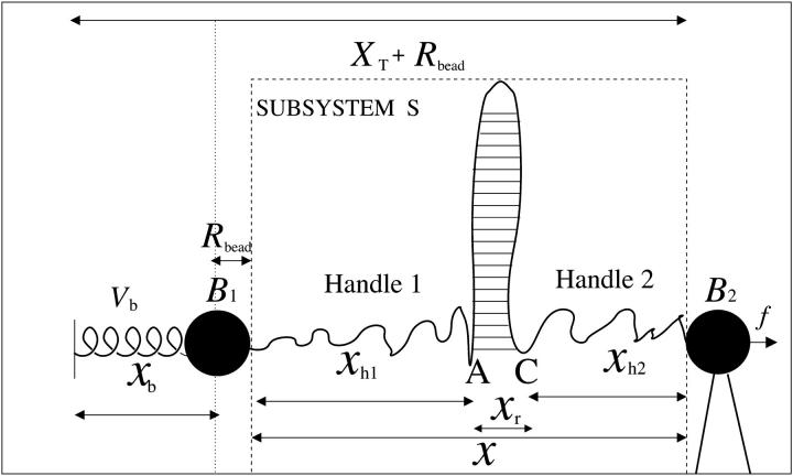
We consider a minimal model to reproduce the experimental setup of a pulling experiment carried out using laser tweezers (Liphardt et al., 2001; Smith et al., 2003). The model (Fig. 1) is composed by a small RNA molecule connected to two polymers called handles, which are used to attach the small RNA molecule to two beads at each end. One bead (B₁) of radius R_bead is confined in the optical trap potential V_b(x) generated by the laser beams. The other one (B₂) is held fixed to the tip of a micropipette by air suction. A micromanipulator controls the position of the micropipette relative to the optical trap. The stiffness of such a glass micropipette is much higher than the stiffness of either the optical trap or the handles; hence we neglect the micropipette-bead fluctuations. The molecule is pulled by moving the micropipette along the x direction. The configurational variables of this simplified system are taken as the projections of the end-to-end distances of each element along the force axis (Fig. 1): for the end-to-end distances of the handles, for the RNA end-to-end distance, and x_b for the position of the bead B₁ in the trap. We use the position x_b of the bead B₁ to read the force f acting on the system, as

(1)

(Note that this is not the way the force is usually measured in dual beam optical tweezers where two photosensitive detectors located at opposite sides of the chamber are used to collect the total amount of deflected light, which is then converted into force after calibration of the machine; see Smith et al., 2003.) To a very good approximation, the optical trap is harmonic. Therefore,

(2)

where k_b is the stiffness of the optical trap. We define the subsystem S as that composed by the two handles and the small RNA molecule. The end-to-end distance for the subsystem S is then given by (Fig. 1). The total distance between the center of the trap and the tip of the micropipette is given by X_T + R_bead = x_b + x + R_bead. Pulling experiments give FECs, f(x), corresponding to the force (Eq. 1) as a function of the end-to-end distance of the subsystem S.

FIGURE 1.

Schematic picture of the model for the experimental setup in an RNA pulling experiment as described in the text. We show the configurational variables of the system x_b, x_r, and which are the projections of the end-to-end distance of each element along the reaction coordinate axis (i.e., the axis along which the force is applied). The potential V_b(x_b) is well described by an harmonic potential for a one-dimensional spring with rest position at x_b = 0.

Ensembles

It is experimentally possible to consider two different ensembles depending on which variable is used as the externally imposed nonfluctuating parameter.

Mixed ensemble

The total distance between the center of the trap and the tip of the micropipette is held fixed, hence X_T is the externally controlled parameter. In this ensemble there are fluctuations in x and f given by Gerland et al. (2003, 2001) as

(3)

where 〈…〉 stands for thermal average, k_B is the Boltzmann constant, T is the temperature of the bath, k_b is the stiffness of the optical trap (Eq. 2), and k_x(X_T) is the effective rigidity of subsystem S. The latter is determined by the serial compliance,

(4)

where (i = 1, 2) and k_r are the rigidities of the handles 1, 2, and the RNA, respectively. These rigidities are X_T-dependent and so are the fluctuations (Eq. 3).

Force ensemble

In this case a piezo actuator controls the force (and therefore the position of the bead B₁). In this ensemble X_T and x are fluctuating variables, 〈δX_T²〉 = 〈δx²〉 = k_BT/k_x(f), where k_x(f) is the stiffness of the subsystem S when the force is held fixed, .

Most of the theoretical work for the force denaturation of RNA in pulling experiments considers the force ensemble. It might be possible to control the force using magnetic tweezers, which allows us to stretch and twist molecules by exerting forces in the range [1fN–10pN]. However, using optical tweezers it is experimentally very difficult to work in the force ensemble where either the force or the variable x_b must be controlled and X_T is a fluctuating variable. To compensate the fluctuations in the force, the distance X_T should be corrected by a feedback mechanism that is difficult to implement. Therefore the most natural ensemble is that where X_T is constant. Indeed, this is the most relevant ensemble for the experiments and therefore we will work in the mixed ensemble throughout this article.

MODELING THE DIFFERENT PARTS OF THE SETUP

Two-states model for a single RNA domain under mechanical load

The unfolding of some biomolecules under the effect of a mechanical force is a highly cooperative process that can be qualitatively described by a two-states model. The two-states model has a long tradition in physics, and has been applied previously by several authors to explain the unfolding behavior of single domains of proteins and RNA hairpins (Liphardt et al., 2001; Ritort et al., 2002; Fernandez et al., 2001; Muñoz et al., 1997; Bokinsky et al., 2003; Zhuang et al., 2000a). Recently, it has been shown how such a simple phenomenological description, with Kramer transition-rates, does not fully reproduce the kinetics observed in pulling experiments of the protein Titin, and more realistic descriptions have been proposed (Hummer and Szabo, 2003).

Let us consider an individual RNA molecule in thermal equilibrium with water solvent (at physiological conditions) at constant temperature, pressure, and zero force. In the simplest description, both states (hereafter denoted by UF, unfolded; and F, folded) are characterized by their Gibbs free energy and respectively, and the RNA molecule occupies each state with a probability given by the Boltzmann distribution. In a more realistic description the molecule can also occupy intermediate configurations, depending on the number n of the first-opened, or denaturated, basepairs (Cocco et al., 2003, Marinari et al., 2002).

When an externally controlled force f is applied to the ends of the RNA molecule, the adequate thermodynamic potential to consider is the Legendre transform of the Gibbs free energy G′(n) = G⁰(n) – fx_r(n) (Tinoco and Bustamante, 2002), where G⁰(n) and x_r(n) stand for the free energy and the projection of the end-to-end distance in the axis force of a hairpin with the first n basepairs opened, respectively. The free-energy landscape G′ is then tilted along the reaction coordinate x_r, which explicitly depends on the number of opened basepairs n. Since we work in the ensemble where neither f nor x_r are control parameters, the nonfluctuating parameter X_T determines the adequate thermodynamic potential The free-energy of the system shown in Fig. 1 is a potential of mean force that characterizes the equilibrium state of the whole system, including the handles, the bead, and the RNA molecule at a fixed value of X_T. 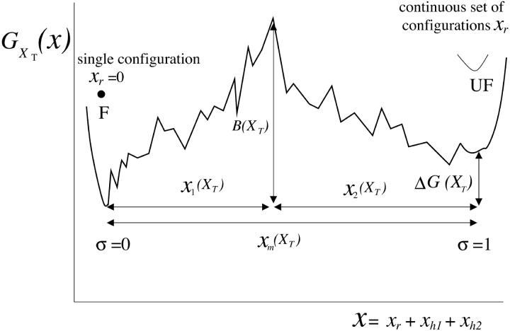The potential free-energy landscape associated to is shown in Fig. 2, where we represent it as a function of the end-to-end distance of the subsystem S, . The shape of the potential shows two pronounced minima corresponding to the F and UF states. The discrete variable σ stands for the state of the domain: the value σ = 0 denotes the F state and σ = 1 the UF state. The relative thermodynamic stability of these states depends on the difference of free energy between them, ΔG(X_T). Moreover, we will consider the existence of a transition state along the reaction path from the F to the UF state and vice versa. This transition state is the RNA configuration with highest free energy connecting the F and the UF states along the reaction path. It may correspond to an RNA configuration where the first n = n* basepairs are opened. (We stress that the shape of the free-energy landscape depends on X_T as well as the location of the barrier corresponding to the transition state. However, for the sake of simplicity, we will assume n* independent of X_T.) In the simplest scenario the transition state can be assumed to have a very short lifetime. Therefore it can be represented by an activation barrier whose main effect is to hinder transitions between the F and UF states. This is the model we will adopt throughout the article. The F and UF states are separated by a barrier of height B(X_T) measured relative to the F state. The barrier is located at a distance x₁(X_T) from the F state and x₂(X_T) from the UF state. The distance between the two states is x_m(X_T) = x₁(X_T) + x₂(X_T). Since the rigidity of the RNA molecule in the F state is very large, we can assume this state to be characterized by a single configuration corresponding to the value x_r = 0 of the reaction coordinate. The RNA in the UF state has a finite rigidity, hence it is represented by a set of configurations within a continuous range of values of x_r (Fig. 2).

FIGURE 2.

Schematic representation of the free-energy landscape, for the whole system at temperature below the melting temperature, for (where is the value of X_T, in which both states F and UF are equiprobable) and normal ionic conditions. For this set of conditions, the stable state is the folded one. In this figure we represent all the parameters characterizing the two-states model. We also show the relevant configurations in the F and UF states along the reaction coordinate x_r: the F state is characterized by a single configuration x_r = 0, whereas the UF state is represented by a continuous set of values of x_r. We use the label σ = 0 for the F state and σ = 1 for the UF state.

Modeling the bead, handles, and the ssRNA

In this section we specify the models for the different elements of the system: the bead trapped in the optical-tweezers potential, the two handles, and the single-stranded RNA (ssRNA) molecule.

Model for the optical tweezers: a bead matched to a spring

We model the optical potential as an harmonic potential of stiffness k_b (Eq. 2); hence the bead in the optical trap can be considered as a bead matched to a spring. We consider that the bead follows a Langevin dynamics of an overdamped particle (i.e., without inertial term),

(5)

where γ (with γ = 6πηR_bead, η, and R_bead being the viscosity of the water and the radius of the bead, respectively) is the friction coefficient and F_R is the resultant force applied to the bead. (In Eq. 5, we are neglecting the drag force felt by the bead, equal to −γv, as the chamber is moved and the water dragged relative to the lab frame at a certain pulling speed For the range of pulling speeds used in the experiments this contribution is negligible, of the order of 0.1 pN.) The stochastic term ξ(t) is a white noise with mean value 〈ξ(t)〉 = 0 and variance 〈ξ(t)ξ(t′)〉 = 2 k_BTγδ(t – t′). The force F_R has two contributions, F_R = f_x – f: the force generated by the optical trap potential, f, given by Eq. 2, and the tension exerted by the subsystem S, f_x. Using the equilibrium condition 〈F_R〉 = 0 or 〈f〉 = 〈f_x〉, and doing an expansion around the equilibrium position of the bead, x_eq, we get

(6)

where k_R is the effective spring constant applied to the bead, k_R = k_x + k_b, with k_x given by Eq. 4. The relaxation time τ_b of the system (i.e., the typical time during which the position of the bead de-correlates) is given by τ_b = γ/k_R.

Polymer model for the handles and the ssRNA

To model the handles and the single-stranded RNA (ssRNA) we use the worm-like-chain (WLC) model. The thermodynamic properties of this model cannot be exactly computed, yet there are useful extrapolation formulas. A simple expression has been proposed (Bustamante et al., 1994) for the force as a function of mean end-to-end distance of the polymer x,

(7)

where L_o and P are the contour and persistence lengths of the polymer, respectively. Equation 7 converges asymptotically to the exact solution as x approaches either zero or L_o and is accurate at least up to 90% in between. Bouchiat et al. (1999) have given an expression with an accuracy of 99% by adding a polynomial of seventh order to Eq. 7. The WLC model works well only at low forces, in the so-called entropic regime, where the molecule behaves as an entropic spring. At high forces there is an enthalpic correction due to the fact that the phosphodiester bonds along the backbone are stretched and the contour length L_o increases. To incorporate this effect it is common to replace x/L_o by x/L_o – f/E_y in Eq. 7, where E_y is the Young modulus of the polymer.

THERMODYNAMIC ANALYSIS

In this section we use the tools of statistical mechanics to analyze the thermodynamics of the system represented in Fig. 1. Most of the analytical treatment is described in the Appendix A. In what follows, we review the main results of these calculations.

Definitions

In equilibrium the observables x_α and their conjugated forces f_α with α = h₁, h₂, r, b (referring to the different elements: handle 1 and handle 2, RNA and bead, respectively) are fluctuating quantities. However, the thermodynamic free energy is only a function of the mean values of these observables that we denote by 〈x_α〉, 〈f_α〉. A representation of 〈f_α〉 versus 〈x_α〉 gives what we call the thermodynamic force extension curve (TFEC) for the element α in the mixed ensemble. If α refers to the whole subsystem S, then the TFEC corresponds to the usual force-extension curve (FEC) recorded in RNA pulling experiments, assuming that the pulling process is carried out reversibly. Throughout the thermodynamic analysis, and to simplify the notation, we will use indistinctly 〈f〉(〈x〉) or f(x) to denote the TFEC. We can also define the restricted average 〈O〉_σ (X_T) as the mean value of the observable 𝒪 when the RNA molecule is in the state σ (i.e., folded or unfolded) for a fixed total end-to-end distance X_T. From now on, all the dependencies of the observables on the variable X_T will not be explicitly written, hence 〈𝒪〉_σ(X_T) ≡ 〈𝒪〉_σ. In Appendix A, we derive an expression for the partition function Z(X_T) corresponding to the system schematically represented in Fig. 1. Applying the saddle point technique, and separating the contributions from the F (σ = 0) and the UF (σ = 1) state we get

(8)

where

(9)

(10)

with Here V_b represents the optical trap potential and ΔG⁰ is the free-energy difference between the F and the UF states at zero force. The function W_α(〈x〉_σ) corresponding to the reversible work performed by adiabatically stretching the element α from 〈x_α〉_σ = 0 to 〈x_α〉_σ = 〈x〉_σ, when the molecule is in the state σ, reads

(11)

where f_α(y) is the TFEC for the element α. The thermodynamic value of any observable 𝒪 can be expressed as

(12)

where p₀ and p₁ are the probabilities for the RNA molecule to be in the F and UF states, respectively,

(13)

At the transition midpoint both states are equally probable,

(14)

where these functions have been defined in Eqs. 9, 10, and 13. Hence, the transition midpoint in the mixed-ensemble is defined by the value of the control parameter that verifies Eq. 14.

Computation of the transition force F^c, the TFEC, and the different contributions to the reversible work

The force at the transition, F^c, is computed as the mean value of the force at given by Eq. 14. To reproduce the experimental results obtained for the P5ab RNA molecule in 10 mM Mg²⁺ (Liphardt et al., 2001) we use the parameters given by Tables 1 and 2 getting F^c = 15.2 pN. This value is close to the one reported from the experiments (Liphardt et al., 2001). We also verify that the value of the computed force at the transition, F^c, is quite stable with respect to changes in the parameters of the problem used to model the handles and the bead, such as the persistence and contour lengths of the handles, the spring constant, and the bead radius. However, because the value of F^c is highly influenced by the characteristics of the RNA molecule, we conclude that the dependence of the value of F^c with the system is basically through the quantities ΔG⁰, L_r, and P_r.

TABLE 1.

Summary table of the parameter values used to model the handles and the bead in the optical trap

kBT[pN/nm]	kb[pN/nm]
4.14	0.1	10	160	1000

We use the value for the Young modulus corresponding to a dsDNA molecule. The value for the other parameters have been taken from Liphardt et al. (2001).

TABLE 2.

Summary table of the parameter values used to model the RNA molecule

Pr[nm]	Lr[nm]		ΔG0[kBT]	N (# pair bases)
1	28.9	800	59	22

We use the value for the Young modulus corresponding to a ssDNA. The value for the other parameters have been taken from Liphardt et al. (2001).

Another interesting magnitude to measure is the reversible work done upon the system when pulling from an initial value X_T = X_T⁰ to a final value of X_T. This work is given by

(15)

where we used Eq. 8. The total reversible work in Eq. 15 defines the change in the free energy of the system. In Fig. 3 A we show the total work and its different contributions, as a function of X_T as derived from the numerical computation of Z(X_T), where the reversible work exerted on each element (handles 1 and 2, bead, and RNA molecule) is defined as

(16)

where

(17)

(18)

(19)

FIGURE 3.

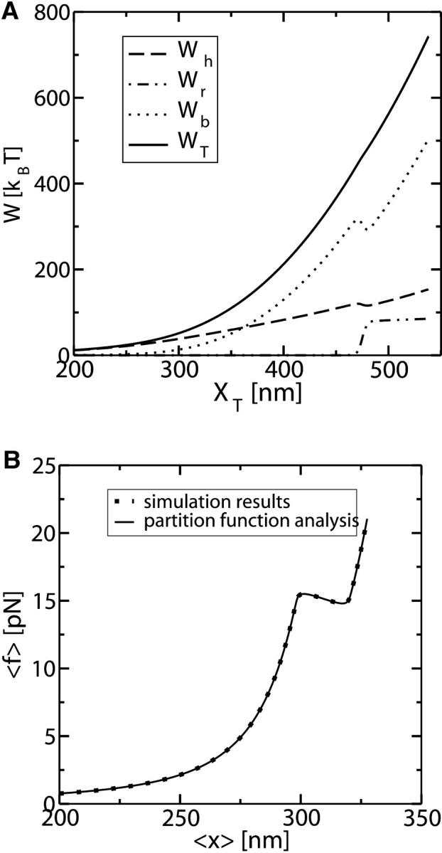
(A) Different contributions to the reversible work obtained from the partition function analysis: as a function of X_T. Note that the smallest contribution to the total work comes from the RNA molecule. (B) The continuous line corresponds to the results obtained from the numerical computation of the TFEC. It is also shown that the TFEC is obtained by averaging over 1000 different trajectories, as explained in Simulation of a Pulling Experiment. The pulling is carried out at an approximate loading rate of 0.5 pN/s, slow enough to generate a quasistatic process. One can observe that both curves agree.

The functions ΔV_b, W_h, and W_r correspond to the change in the potential energy of the bead in the optical trap and the work exerted upon the handles and the RNA molecule by moving the total end-to-end distance from the initial to the final value of X_T, respectively. Finally in Fig. 3 B we represent the TFEC for the subsystem S, 〈f〉 versus 〈x〉. This is obtained by numerical computation of the partition function using the relation

(20)

To calculate 〈f〉 we use the expression (Eq. A1) for the partition function of the system Z(X_T). Integrating this expression over the bead position x_b gives

(21)

where Z^α(x_α) is the partition function of the element α, with α = h₁, h₂, r, and b. The partition function for the bead (Eq. A2) satisfies

(22)

where we used Eq. 2. Therefore the absolute value of the mean force, Eq. 20, can be computed as

(23)

where The generalized force, Eq. 20, is the average force measured in the optical trap.

Reversible work across the transition

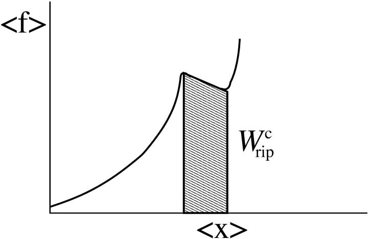
The quasistatic work exerted upon the subsystem S across the transition is the area under the TFEC (Fig. 4), 〈f〉(〈x〉), from the folded branch 〈x〉 = 〈x^c〉₀ (σ = 0) to the unfolded branch 〈x〉 = 〈x^c〉₁ (σ = 1) (see Appendix A), where the super-index c indicates that the system is at the transition midpoint, (Eq. 14),

(24)

FIGURE 4.

The shadow area under the TFEC along the transition corresponds to the quasistatic work (schematic representation).

At the transition midpoint, both states are equally populated and Eq. 14 holds. Therefore identifying Eqs. 9 and 10, we can write Eq. 24 as

(25)

where the functions with a super-index c are evaluated at the mean value of their variables at the critical extension The value W_r, given by Eq. 11, is the loss of entropy of the RNA molecule along the transition due to the stretching. The value ΔW_h is the free-energy change of the handles between the folded and unfolded branches, and is given by

(26)

Equation 25 tells us that the quasistatic work coincides with the change of free energy of the different elements that form the subsystem S across the transition. The value is experimentally measurable as the area under the rip observed in the TFEC corresponding to the F–UF transition (Fig. 4). Therefore Eq. 25 provides a way to estimate the unfolding free energy of the molecule ΔG⁰ from the TFEC, which is a quantity biologically relevant as it determines the direction of biochemical reactions. This free energy ΔG⁰ is equal to the Gibbs free energy measured by thermal denaturation in bulk experiments extrapolated to the working temperature.

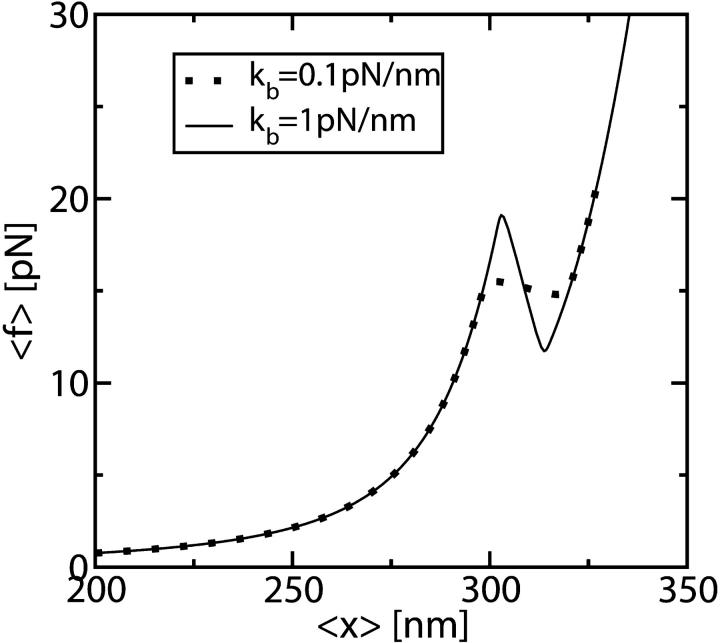
In Fig. 5 we show two TFECs obtained from the partition function analysis corresponding to two systems with different k_b but with the same handles and RNA molecule with parameters given in Tables 1 and 2, respectively. We use Eq. 25 to extract the value of ΔG⁰ by computing as the area under the rip in the TFEC (Fig. 4). As expected for an harmonic trap (Eq. 2), the TFEC in Fig. 5 shows an slope at the transition (rip) proportional to −k_b. To obtain the different contributions to Eq. 25 we first use the WLC model (Bouchiat et al., 1999) to estimate and given by Eqs. 11 and 26. Finally, we compute the area under the TFEC across the transition (rip) to obtain and use Eq. 25 to extract ΔG⁰. The results are given in Table 3. 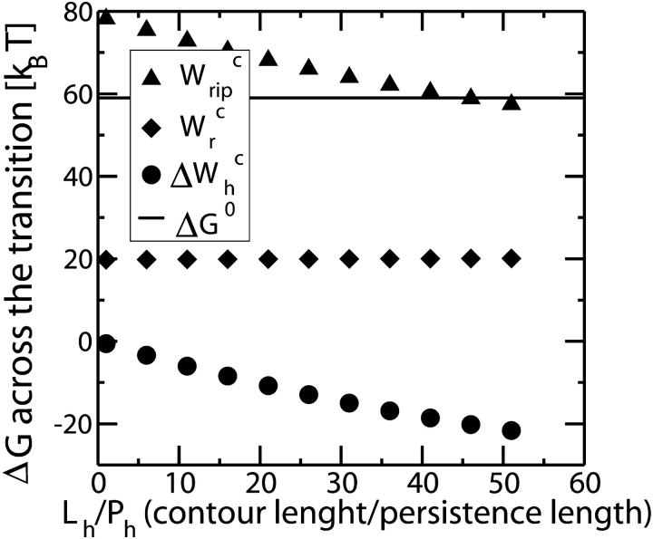Note that the contribution is negative because when the RNA molecule opens the force relaxes and the handles contract, hence the free energy of the handles across the transition decreases. Neglecting the contribution that comes from the handles across the transition is a typical approximation often applied to experimental results. However, this is not always accurate as this contribution can be large. In the previous example, even in the case of small k_b, we would lose 8 k_BT in the balance equation (Eq. 25). In Fig. 6 we show, for a small value of k_b (k_b = 0.1 pN/nm), how the different contributions to Eq. 25 change when considering systems with different values for the ratio L_h/P_h. The stretching contribution to the UF state of the RNA, does not change when modifying the magnitude L_h/P_h, because the forces at which the transition occurs are quite stable under changes of L_h/P_h. However, the magnitude of the contribution tends to notably increase as L_h/P_h becomes larger.

FIGURE 5.

TFEC corresponding to two systems with handles and RNA characterized by the parameters given in Tables 1 and 2 and with an optical trap stiffness k_b = 0.1 pN/nm and k_b = 1 pN/nm, respectively. Note that the slope of the TFEC at the transition (rip) is proportional to −k_b.

TABLE 3.

Different contributions to the free-energy change across the transition

kb[pN/nm]
0.1	20	−8.5	70.5	59
1	17	−41	35	59

As expected, the value of ΔG⁰ is independent of the other parameters of the system.

FIGURE 6.

The different contributions to the free-energy change across the transition presented as a function of the ratio L_h/P_h. Note that the value of ΔG⁰ is independent of that ratio (see also Table 3).

SIMULATION OF A PULLING EXPERIMENT

To simulate a pulling experiment it is important to distinguish the different timescales involved in the problem. Typically the bead has a much bigger size than the other components of the system (handles and ssRNA), therefore the bead is the element with largest dissipation and slowest relaxation compared to the elastic and bending modes of the handles and the ssRNA: τ_b ≫ τ_handles, τ_ssRNA. The characteristic time τ_b at which the bead relaxes to its equilibrium position can be computed as the ratio between the friction coefficient of the bead γ and the effective spring constant applied to the bead k_R = k_x + k_b (see Eq. 6), with k_x given by Eq. 4, i.e., τ_b = γ/k_R. For the typical experimental values for the trap stiffness and the radius of the beads, k_b ≈ 0.05–0.15 pN/nm and R_bead ≈ 1–3 μm, the time τ_b lies in the range [10⁻³ s–10⁻⁶ s]; its value depends upon the value of the control parameter X_T. The characteristic time τ_F–UF at which the RNA hairpin folds and unfolds depends on the sequence of bases and also on the presence of tertiary contacts that slow down the kinetics of the unfolding reaction. Typical values are of the order of seconds-to-milliseconds. Hence the dynamics of the system shows the following separation of timescales: τ_F–UF ≫ τ_b ≫ τ_handles, τ_ssRNA. Therefore we can consider an instantaneous relaxation for the handles and the bead to solve the dynamical equations that describe the folding-unfolding kinetics of the RNA molecule. This hypothesis is valid, as long as the data is collected at frequencies smaller than the relaxational frequency of the bead, which is the element with the largest relaxation time. The dynamics for the RNA molecule is governed by a master equation for the probability p_σ (Eq. 13),

(27)

The functions k_→ and k_← are the unfolding and folding rates corresponding to the activated process schematically represented in Fig. 2,

(28)

where k₀ is an attempt frequency. These rates satisfy the detailed balance condition,

(29)

The expressions of ΔG(X_T) and B(X_T) are derived in Appendix B using the partition function analysis.

To simulate a pulling experiment we use an adiabatic approximation by taking advantage of the great separation of timescales between the folding-unfolding kinetics and the relaxational dynamics of the different elements of the system. At each value of the extension X_T and for a given state of the RNA molecule (σ = 0, 1) we determine the values of the mean extension and force for the bead, handles, and ssRNA using the equilibrium equations. At the same time we numerically solve the dynamics for the RNA molecule (Eq. 27). In what follows, we describe the steps of the algorithm:

Step 1. We increase X_T by vΔt, where v is the pulling speed, i.e., the velocity at which the micropipette is pulled, and Δt is the iteration time, hence is the frequency at which data is collected. Note that the relation between the pulling speed v and the loading rate r, i.e., the velocity at which the force increases, can be found using the relation between the force and displacement increments, Δf = k_eff(f)ΔX_T, as

(30)

where k_eff is the effective stiffness of the system, computed as

(31)

and where k_x has been defined in Eq. 4 and k_b is the stiffness of the optical trap. The F–UF transition for a small single RNA domain typically occurs at forces in the range 8–20 pN. At these forces the system verifies that k_b is much smaller than the stiffness of the handles and the RNA molecule, and k_r; and therefore we can safely take v = r/k_b.

Step 2. We compute the new 〈f〉 and 〈x〉 iteratively, using the saddle point equations for the partition function. To these mean values we add Gaussian fluctuations of zero mean and variance given by Eq. 3. We then obtain the FEC, f(x), which should qualitatively reproduce the experimental one.

Step 3. The RNA molecule is then unfolded or folded, with a probability k_→(X_T)Δt or k_←(X_T)Δt, respectively, where Δt is the iteration time. For the rates, we use Eq. 28 with the functions ΔG(X_T) and B(X_T) given by Eqs. B2 and B3, respectively.

Force-extension curve results (FEC)

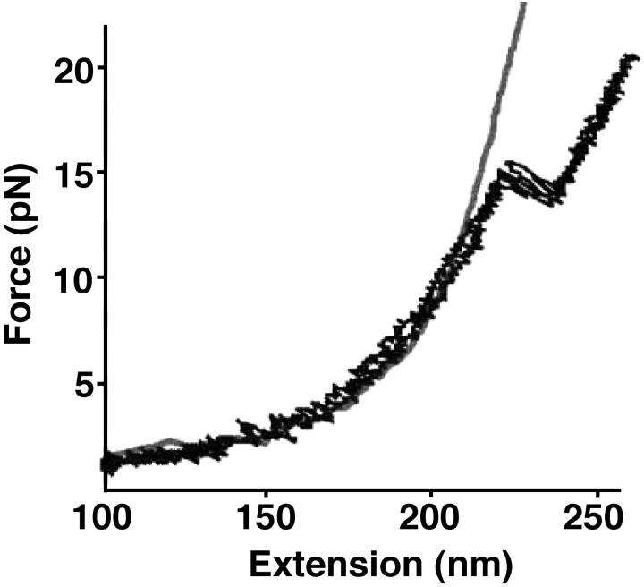
In Fig. 7, A and B, we show the resulting FEC of our simulations for the values used in the experiment of Liphardt et al. (2001) shown in Tables 1, 2, and 4, corresponding to a P5ab RNA molecule and for a loading rate of r = 1 pN/s and of r = 50 pN/s, respectively. In these simulations we implement the dynamical algorithm previously described for the forward and reverse processes where X_T increases and decreases in time, respectively. As shown in Fig. 7 A, at a loading rate of 1 pN/s, different transition jumps are observed along both the forward and reverse processes, because the pulling speed (v) is low enough. Comparing these simulation results with the experimental FEC (Liphardt et al., 2001) shown in Fig. 8, we find a qualitative agreement, and the shape of the curve around the transition region is qualitatively reproduced. However, we find some discrepancies:

1. The simulated curve is shifted in the x direction in comparison with the experimental one. This is because, experimentally, the quantity measured is the relative change in x rather than its absolute value. Indeed, there may be some uncertainty (typically of the order of 100 nm) in the diameter of the bead used in the experiments. The value of the diameter is required to determine the distance x from the experimentally measured value of the distance between the centers of the two beads (equal to x + 2R_bead). Therefore, in Fig. 8, the extension represented in the x axis corresponds to changes in the value of x with respect to an initial extension of ∼100 nm.

2. As the force increases, the experimental curve separates from the theoretical WLC prediction and therefore from the simulated results. The agreement can be improved by considering larger values for the Young modulus of the handles and of the ssRNA. Furthermore, by extending the RNA molecule model to include intermediate configurations, which depend on the number of opened basepairs n, we realize that the cooperative transition might not be between the F (n = 0) and UF (n = N) states, but between partially folded and partially unfolded states. For instance, for the P5ab RNA molecule, the cooperative folding-unfolding transition is between the state n = 3 and the state n = N (Cocco et al., 2003). This means that typically the first three basepairs open before the transition occurs, increasing the extension of the handles.

FIGURE 7.

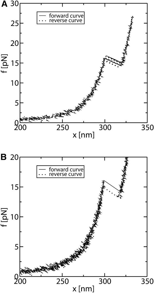
Results for the FEC obtained from the simulation of a pulling experiment with iteration time Δt = 10⁻² s. (A) Pulling rate r = 1 pN/s. (B) Pulling rate r = 50 pN/s. At this pulling rate the molecule is driven out of equilibrium, and hysteresis is observed around the transition.

TABLE 4.

Parameters used to characterize the kinetics of folding-unfolding of RNA

k0 exp(– βB0)	n*
e−30 ≈ 10−13	12

They are chosen to reproduce the experimental kinetics results obtained with the hairpin P5ab (Liphardt et al., 2001). The n* is the number of basepairs opened in the transition state.

FIGURE 8.

Experimental FEC for P5ab obtained in experiments carried out by Liphardt et al. (2001) The continuous line corresponds to the WLC curve for the handles. Figure is taken from Liphardt et al. (2001).

Fig. 7 B shows the FEC corresponding to a pulling process carried out at a loading rate of r = 50 pN/s. At this pulling speed, the process is not in equilibrium, and hysteresis effects are observed around the transition region.

Fraction of trajectories that have at least one refolding

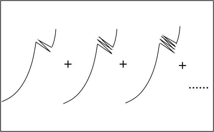
We consider a system with a control parameter (generally denoted by y) that is pulled by changing y at certain speed . The forward (reverse) pulling process starts at a initial value of the control parameter y_i (y_f) where the RNA is in the F (UF) state and finishes at a final value of the control parameter y_f (y_i) where the RNA is in the UF (F) state. We then define N_F and N_R as the fractions of forward and reverse trajectories that have at least one refolding, respectively (Fig. 9). These fractions are given by

(32)

(33)

where the first integral in the right-hand side of both equations accounts for the probability of unfolding (folding) before a certain value of the control parameter y is reached and the second integral accounts for the probability of refolding once the RNA molecule has been unfolded (folded). The function ρ_σ^F(R)(z, z′) is the probability that the RNA molecule remains at the state σ until y = z′ starting at y = z in the forward (reverse) process. The term ρ_σ is the solution of the master equation:

(34)

(35)

with initial condition In Appendix C we prove that the fraction N_F is equal to N_R if the perturbation protocol for the control parameter is symmetric, i.e., if the velocities along the forward and reverse process verify v_F(y) = – v_R(y). In our analysis the control parameter y corresponds to the total distance X_T and the folding-unfolding rates are given by Eq. 28. The detailed analytical expressions for the rates have been given in Eqs. B5 and B6. Analytical computations with such rates appear quite cumbersome and it is preferable to simplify them. For analytical purposes, we will consider effective rates where the functions B¹ and ΔG¹ given by Eq. B7 and x₁ and x₂ (the distances from the F and UF states to the transition state along the x axis, see Fig. 2) are effective parameters independent of X_T. We call these obtaining

(36)

where the force f_σ (σ = 0, 1) is the force acting upon the system at a given value of X_T when the RNA is in the state σ. (The approximation expression in Eq. 36, where force does not fluctuate near the transition, is well justified. In fact, when the RNA is in a given state, i.e., folded or unfolded, the magnitude-of-force fluctuations is negligible, with the RMS in the range 0.03–0.1 pN, so one can consider the instantaneous force equal to the mean force. Hence the fluctuations in force near the transition arise solely from the force jump between the F and UF states.) The forces f₀ and f₁ in Eq. 36 correspond to the two branches (Eq. A16): f₁ = k_b(X_T – 〈x〉₁) and f₀ = k_b(X_T – 〈x〉₀), where we used Eq. 23. Therefore, the relation between f₀ and f₁ reads as

(37)

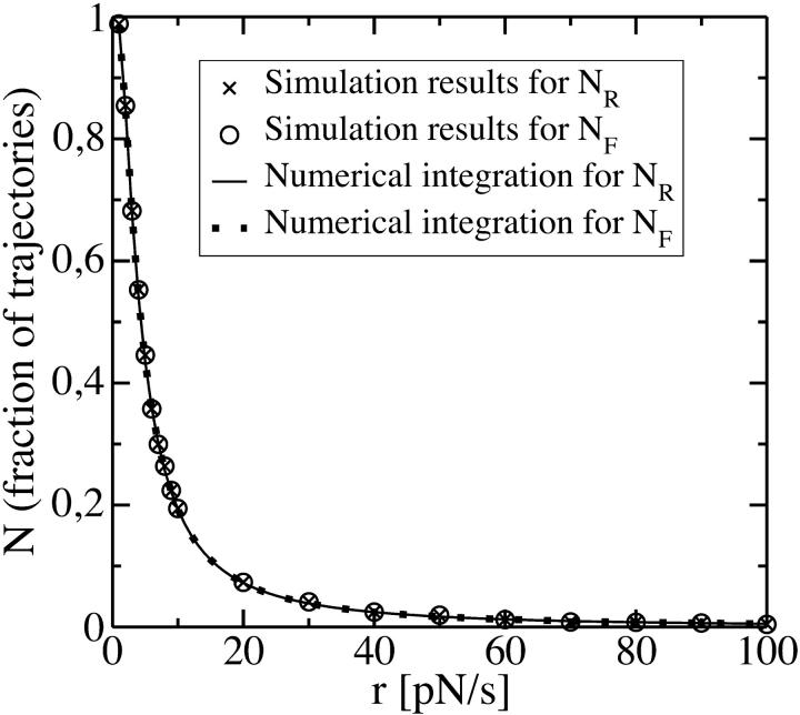
where is the distance between the F and UF states along the x axis, . Using Eq. 37, it is straightforward to see that the effective rates (Eq. 36) satisfy the detailed balance condition (Eq. 29). We can now compute the fractions (Eqs. 32 and 33) as a function of the loading rate r. In Fig. 10, we show the results obtained for the fractions N_F and N_R from the numerical computation of Eqs. 32 and 33, using the effective rates (Eq. 36) with the definitions in Eqs. B5–B7. We also show the results obtained from the simulations for the fractions N_F and N_R as a function of the loading rate r, and they agree fairly well.

FIGURE 9.

Different trajectories that have at least one refolding. The ratio between the sum of these trajectories and the total number of trajectories gives the fraction N_F for the forward process and N_R for the reverse process.

FIGURE 10.

The fractions N_F and N_R as a function of r. Simulation results correspond to 5000 realizations of a pulling experiment. We also show the numerical integration of Eq. 32 (equal to Eq. 33; see Appendix C) using the rates (Eq. 36) with the following parameters:

From these simulations we can also compute the mean work exerted upon the system as a function of r,

(38)

where f_i is the force acting on the system (Eq. 2), ΔX_T is the uniform increase in the total end-to-end distance at each iteration, and n is the total number of iterations. The average is over different realizations of the simulation of the pulling process. The total mean work is the sum of the reversible work (i.e., the work measured in a quasistatic process, r → 0), and the mean dissipated work,

We then consider the fraction N_F(r) for three different RNA molecules characterized by different parameters, i.e., ΔG⁰, L_r, N (total number of basepairs), n*, and B⁰ ln k₀; the results are shown in Fig. 11 A. Plotting these fractions N_F as a function of the mean dissipated work 〈W_dis〉 exerted upon the system, we find that the three curves corresponding to the three RNA molecules show the same kind of dependence (Fig. 11 B). This dependence is not surprising as the average dissipated work has been already shown (Ritort et al., 2002) to be a useful quantity to characterize the non-equilibrium regime. In particular, in the linear response regime, the average dissipated work depends linearly on the loading rate r, the proportionality constant being a function of the relaxation time of the molecule, the unfolding free energy, and the transition force (Ritort et al., 2002). The collapse of all curves in Fig. 11 is, however, not restricted to the linear response regime. Indeed, we have verified that in the regime 2 k_BT < 〈W_dis〉 < 5 k_BT, where deviations from the linear response regime are observable (Fig. 12), there is still a good collapse in Fig. 11 B of the curves corresponding to the three molecules. Note that by measuring the fraction N_F we can obtain information about the value 〈W_dis〉, and from the knowledge of the total work we can extract the reversible work exerted upon the system. This provides an alternative way to derive equilibrium information from non-equilibrium experiments (Liphardt et al., 2002; Ritort, 2003).

FIGURE 11.

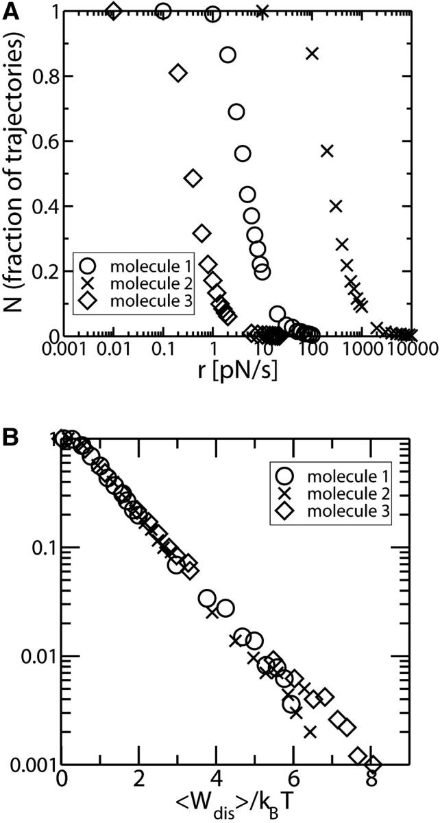
(A) The fraction N_F as a function of r for three different RNA molecules characterized by Molecule 1, ΔG⁰ = 59 k_BT; L_r = 28.9 nm; N = 24; n* = 12; and B⁰ ln k₀ = 29 k_BT. Molecule 2, ΔG⁰ = 89 k_BT; L_r = 40 nm; N = 34; n* = 15; and B⁰ ln k₀ = 45 k_BT. Molecule 3, ΔG⁰ = 39 k_BT; L_r = 16.5 nm; N = 14; n* = 9; and B⁰ ln k₀ = 19 k_BT. (B) The fraction N_F as a function of 〈W_dis〉 in logarithmic scale for the three RNA molecules considered in a (upper panel). Data collapse in a single curve.

FIGURE 12.

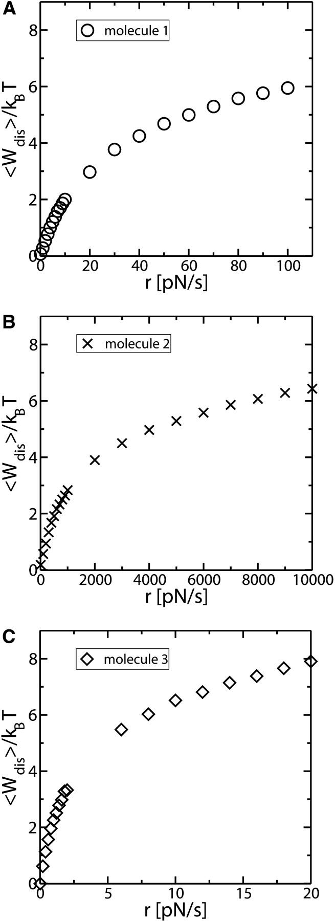
Mean dissipated work as a function of the loading rate r for Molecule 1 in A, for Molecule 2 in B, and for Molecule 3 in C. The characteristics for the three molecules are given in Fig. 11. Note that the regimes studied are far from the linear response regime, as the curves deviate from straight lines. Deviations from the linear response regime arise in the range of r-values where the fraction N approaches zero (Fig. 11 A).

UNFOLDING OF DOMAINS STABILIZED BY Mg²⁺ TERTIARY CONTACTS

In this section we will focus on the unfolding kinetics of molecules that form tertiary contacts induced by magnesium ions (Mg²⁺). Experiments on the unfolding kinetics of domains stabilized by Mg²⁺ tertiary contacts show how intermediate states are characterized by high barriers that are located close to the folded state along the x axis (Liphardt et al., 2001; Onoa et al., 2003), x₁ ≪ x_m (Fig. 2). (Studies by Imparato and Peliti, 2004, suggest that the domains stabilized by Mg²⁺ tertiary contacts are better characterized by kinetic models with more than one barrier. Here we just consider the simpler case of a single barrier per domain.) According to Eq. B3, when the force acting upon the folded molecule, 〈f〉₀, increases, the barrier B(X_T) decreases proportionally to the distance x₁. Consequently, for small x₁, the height of the barrier B is quite insensitive to the force (or X_T), meaning that when the force exerted upon the system increases, B decreases much slower than the difference of free energy between both states, ΔG. Therefore big barriers and small values of x₁ imply slow unfolding processes. In complex RNA molecules the domains stabilized by the presence of Mg²⁺ tertiary contacts are rate-limiting for the unfolding of the whole molecule (Zarrinkar and Williamson, 1994; Fang et al., 2002; Russell et al., 2002b; Zhuang et al., 2000b). In these conditions, even at very low loading rates, the probability of refolding, once the domain is unfolded, is almost zero. The unfolding of RNA molecules with Mg²⁺-dependent barriers at experimental loading rates (r ≈ 3–5 pN/s) becomes a “stick-slip” process (Onoa et al., 2003). Therefore, we can use the transition rates

(39)

with B(X_T) given by Eq. B3. These rates have been considered by Evans and Richie (1997, 1999) in the study of bond failure. (Note that these rates do not verify the detailed balance condition.)

In the previous analysis we have considered the study of single-domain RNA molecules. Now we want to analyze molecules that have more than one domain. To this end, we extend the model developed in preceding sections to describe more complex RNA molecules.

Domains with Mg²⁺-dependent barriers that unfold sequentially under a loading rate

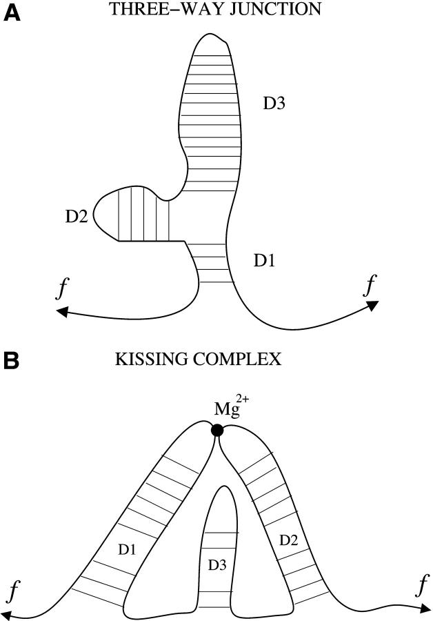
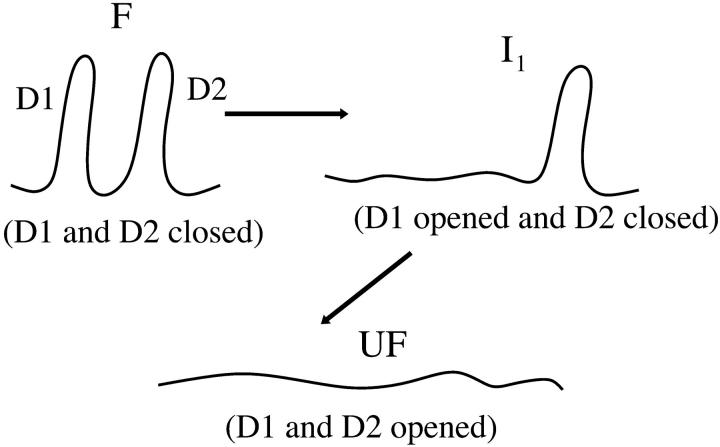
In this section we want to investigate the applicability of the model developed in previous sections to more complex RNA molecules, such as a multidomain RNA molecule with sequential unfolding of its domains under the effect of an external force. There are two situations that favor a sequential unfolding of the domains. First, the topological connectivity of the molecule does not allow certain domains to unfold, before certain others have not yet opened (Fig. 13 A). The second one is the blockade of the force induced by the most external tertiary contacts on the interior domains (Fig. 13 B). For the sake of clarity, we will consider a sequential unfolding of a multidomain RNA molecule. In general, the unfolding of domains is a hierarchical process that is not necessarily sequential. For instance, in Fig. 13 A, once D1 has opened, either D2 or D3 can be unfolded. However, in our modelization we assume that D2 and D3 unfold in a given sequential order (e.g., first D2 and later D3). The motivation to consider this simplified model is twofold. On the one hand, there are experimental results on the molecule L-21, a derivative of the Tetrahymena thermophila ribozyme, where the order of the opening of the different domains of the molecule studied was never observed to change (Onoa et al., 2003). On the other hand, there might be RNA complexes in which the different domains typically unfold at forces that differ significantly (few pN), in such a way that unfolding of the complex is almost always sequential. A main goal throughout this article is to illustrate how the model for the experimental setup previously introduced can be generalized to include complex RNA molecules (and not only hairpins), rather than emphasizing details of the modeling of the RNA structure. With this proviso, we model the RNA molecule as an unidimensional chain of single domains connected in series, each one represented as a two-states model. For an n-domain system we have the F state, the UF state, and the n–1 intermediate, I_i, where i stands for the index of the intermediate (Fig. 14).

FIGURE 13.

Different mechanisms for the blockade of the force. (A) Blockade of the force for certain domains (such as a three-way junction molecule) due to the connectivity of the molecule. The force cannot act upon the domains D2 and D3 while D1 is closed. (B) Blockade of the force for certain domains (such as an RNA kissing complex) due to the presence of Mg²⁺ tertiary contacts. The domain D3 does not feel the force until the Mg²⁺ tertiary contact breaks.

FIGURE 14.

Representation of the different states for a two-domain model corresponding to a molecule with two domains that sequentially unfold. The kinetic parameters of each domain are where the super-index i = 1, 2 refers to the index of the domain.

We simulate a pulling process without refolding using the effective unfolding rate given in Eq. 36 for a molecule with three domains in series. This system could represent the domain P4–P6 of the molecule L-21, recently investigated (Onoa et al., 2003), in which a sequential unfolding of the domains was observed. Although sometimes two domains open simultaneously, the most frequently observed pathway contains three transitions corresponding to the consecutive opening of the domains P4P6, P5, and P5abc. In Fig. 15 we show the FEC of a three-domain RNA system, and in Fig. 16 the histograms for the starting position of the rips detected. The results shown in Figs. 15 A and 16 A have been obtained by doing a numerical simulation of a pulling experiment using the parameters for the handles and the bead given in Table 1. The kinetic parameters of each RNA domain are given in the caption of Fig. 15. In Figs. 15 B and 16 B, we show the experimental results (Onoa et al., 2003). For the third domain, which corresponds to the well-known domain P5abc, we use the values of the parameters obtained by Liphardt et al. (2001). We choose the parameters for the other domains to qualitatively reproduce the experimental results for the unfolding trajectories (Onoa et al., 2003) shown in the lower panel of Fig. 15. There are some differences between the histograms obtained from the numerical results and the experimental ones (Fig. 16). The main differences are observed in the height at the peak corresponding to the third domain and the amplitude of the fluctuations of the position where each domain opens. Both are smaller in simulations as compared to experimental results. (Note that in the experimental results the distances are given in units of nucleotides. Our results are obtained in nanometers and then transformed to nucleotides by using an approximative conversion unit of 0.45 nm per nucleotide, which corresponds to the conversion between ssRNA length in nanometers and nucleotides when the force exerted upon the molecule is 15 pN.) Several reasons can explain this disagreement. First, there are strong drift effects in the machine that introduce instrumental noise. Second, no two pulled molecules give identical FECs; this could be explained by the disparity of the attachments, with existence of more than one molecule on the bead that can influence force measurements. Third, the RNA molecule is not just composed by a series of domains, but there are other regions (some bases) that do not belong to any domain. These regions can contribute differently to increase the length of the rips, a source of randomness for the position of the start of the rips. Last but not least, we cannot exclude the possibility that the kinetic model we are considering is too simple to explain the unfolding of these domains. Actually, it is known that complex RNA structures show characteristic FECs that cannot usually be interpreted in terms of the successive opening of native domains, because of the existence of long-lived intermediates including non-native helices (Harlepp et al., 2003).

FIGURE 15.

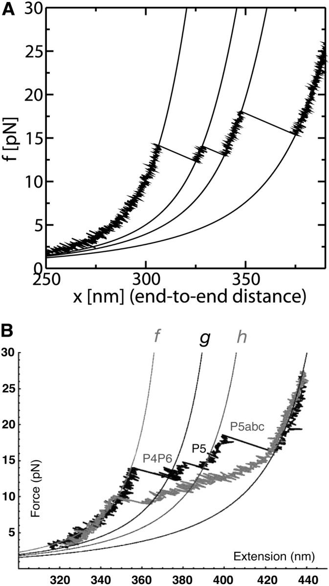
Comparison of FECs between model and experiments. (A) Numerical simulations of the pulling process at r = 4 pN/s for a three-domain RNA molecule. Simulations have been done with the effective model Eq. 36 without refolding. Domains are characterized by the following parameters: Domain 1, ; Domain 2, ; and Domain 3, where the super-index refers to the index of the domain. The solid lines correspond to the WLC force-extension curves. (B) Experimental FEC for the P4–P6 domain obtained by Onoa et al. (2003). The solid lines correspond to WLC curves for the handles linked to the RNA molecule. (Note that the lower curve corresponds to a refolding process we do not consider here.) Figure taken from Onoa et al. (2003).

FIGURE 16.

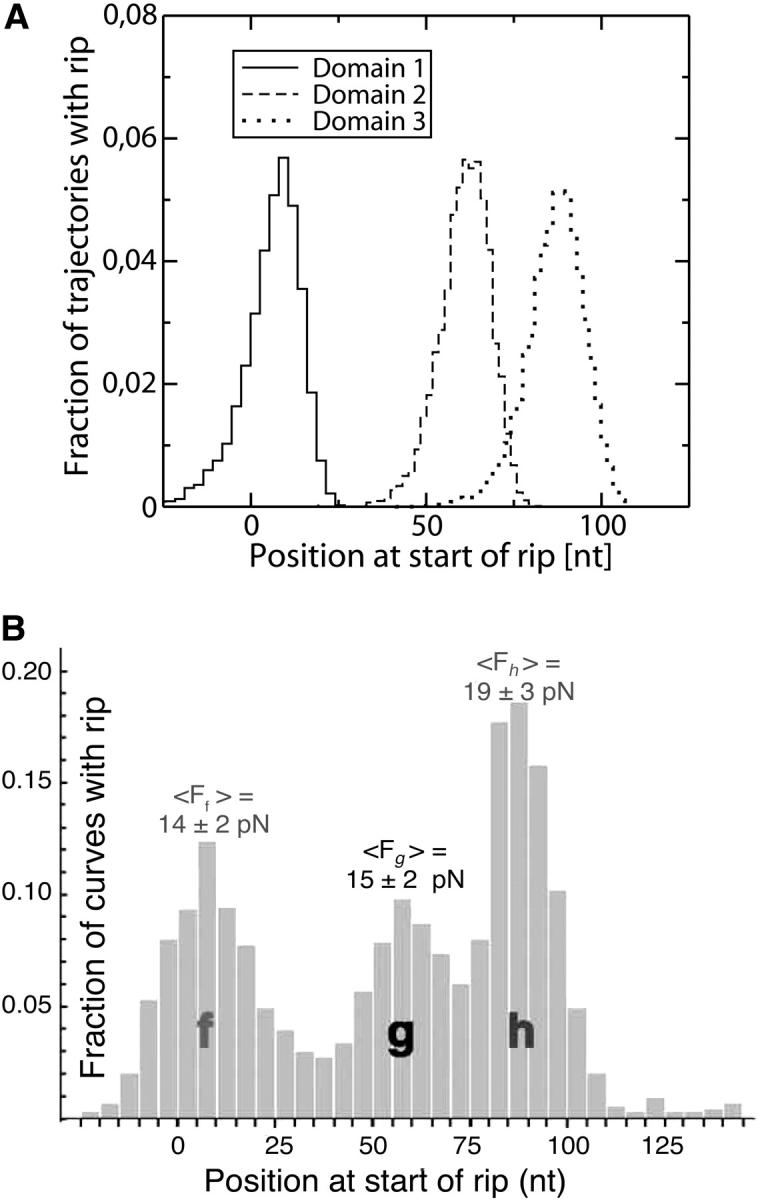
Comparison between model and experiments of the rip position distribution. The position of the rip (abscissa) is represented in units of nucleotides. (A) Histograms for the positions at the start of the detected rips obtained from the simulation. They correspond to the three transitions observed in Fig. 15 A. The parameters used in the simulation are given in Fig. 15 A. (B) Experimental histograms of rips detected in 732 unfolding curves of P4–P6 (Fig. 15 B). Figure taken from Onoa et al. (2003).

CONCLUSIONS

The recent fast development of nanotechnologies allow scientists to investigate the physical behavior of complex biomolecules. Of particular importance are those physical processes in the nanoscale where the typical values of the energies involved are several times k_BT. In such regimes, fluctuations and large deviations from the average behavior are important and deserve a careful investigation as they can contribute a lot to the understanding of thermal processes in small systems. RNA pulling experiments offer an excellent framework to address such questions as RNA molecules can be small enough for stochastic fluctuations be observable and measurable.

A very useful technique for manipulating individual molecules is that of the optical tweezers, a technique covering a range of forces 1–100 pN, which is relevant for many biological processes. A full understanding of how to extract accurate physical information from such experiments is therefore of great importance. The present work represents an attempt in that direction. At present it is not yet possible to unfold individual RNA molecules without attaching some polymer handles at their extremes, therefore all RNA pulling experiments are carried out with a system larger than the individual naked RNA molecule. This system includes the RNA molecule, the polymer handles, and the bead in the optical trap. To extract accurate physical information regarding the RNA molecule, a global treatment of the whole system is necessary.

In this article we analyzed the minimal system required to interpret the data extracted from RNA pulling experiments. We did not include any details regarding the response of the machine or a realistic and accurate modelization of the structure of the RNA molecule. A key part of our treatment is a proper consideration of the ensemble relevant to pulling experiments. Although the end-to-end distance (between the bead and the micropipette) and the force are variables that fluctuate, the total end-to-end distance X_T (Fig. 1) does not. The thermodynamic potential in such an ensemble is the key quantity that allows us to extract accurate knowledge of the influence of these external parts (beads and handles) on the thermodynamic and kinetic behavior of the RNA molecule.

We focused on small RNA hairpins that show cooperative unfolding, and we verified that the simple model studied qualitatively reproduces the results reported from experiments (Figs. 7 and 8). By analyzing the thermodynamics of the whole system, first, we get an explicit expression (Eq. 14) for the transition force F^c as well as the TFEC (see Eq. 23); and second, we get a relation between the unfolding free-energy of the molecule ΔG₀ and the area under the force rip (see Eq. 25), which is an experimentally measurable quantity. Taken together, these results establish a framework to infer thermodynamic properties of the RNA molecule from the experimental data. Moreover, they also allow us to understand the conditions (parameters for the bead and handles) under which it is most reliable to get estimates for these properties. From the study of the dynamics of the pulling process we find a generic relation between the fraction of molecules that unfold (refold) at least twice during the unfolding (refolding) process and the mean dissipated work. This relation could allow us to extract the reversible work for the unfolding process by using data extracted from non-equilibrium pulling experiments. This procedure is reminiscent of other techniques, recently applied to RNA pulling experiments (Liphardt et al., 2002), based on the Jarzynski equality or similar relations (for a recent review, see Ritort, 2003). Moreover, we have shown a symmetry property that relates these fractions for the forward and reverse processes. How general this result is in transition state theory (Bolhuis et al., 2002), i.e., beyond the case of a cooperative two-states system, remains an interesting open question. To stress the adaptability and feasibility of our model to describe more complex type of molecules, we have also considered the unfolding of a large RNA molecule made out of different domains that unfold sequentially. The unfolding of these domains is controlled by Mg²⁺ tertiary interactions which induce large energy barriers, thereby a refolding event (while the molecule is pulled) is not observed at experimental conditions. Although our study is not complete for such molecule types (the assumption of a sequential unfolding may not consider other possible unfolding pathways), it is instructive to see that by modifying only the model for the RNA molecule we are still capable of qualitatively reproducing several experimental results, as shown in Figs. 15 and 16.

How to choose the characteristics of the components of the experimental setup, such as the stiffness of the trap, the bead radius, the contour length, and the persistence length of the handles, to extract reliable information about the hairpin? This may not be an easy question to answer. The main difficulty lies in the high level of complexity and nonlinearity of the system studied. To illustrate such difficulty let us consider what would be if we were to use much stiffer traps (such as the atomic force microscope). In this case, fluctuations in the force measured f are larger, but fluctuations in the distance between the two beads x are smaller (see Eq. 3). Therefore, to obtain a force-extension curve with the minimum noise it would be desirable to work in an intermediate regime where neither the fluctuations in f nor x are too large. On the other hand, by considering stiffer handles (shorter contour length or larger persistence length, e.g., carbon nanotubes) the amplitude in the fluctuations either in f or x decreases. Hence, the optimal conditions would suggest us to use handles that are as stiff as possible. However, the force measured f is not the same as the instantaneous force exerted upon the RNA molecule f_RNA (they are equal in mean value but, because they fluctuate, their instantaneous values differ). The fluctuations in f_RNA are of the order of (where 〈δx²〉 is given in Eq. 3). If the goal of the experiment is to control the value of the force f_RNA exerted upon the molecule (as it is the case in force-feedback hopping experiments), one may prefer to work with handles as flexible as possible.

Many aspects of RNA pulling experiments are still open. Among these: it would be interesting to extend these considerations to include more complex effects induced by the response of the machine; experimentally test some of the results predicted in this work for the fraction of unfolded events; and to conduct a detailed investigation of the kinetics of the folding process (rather than the unfolding) in the presence of force, a process for which we still lack an understanding. Several of these aspects will be addressed in the near future.

APPENDIX A: PARTITION FUNCTION IN MIXED ENSEMBLE

The partition function, Z(X_T), for the system described in Fig. 1, gives the free energy as well as other relevant thermodynamic properties. The state of the system is defined by the externally controlled variables X_T, T, and P. The last two, T and P, are always kept at a constant value so we can ignore them throughout the article. The partition function for this one-dimensional system can be written as the convolution of the contributions coming out from the different elements,

(A1)

where is the partition function distribution of the element α, with α = h₁, h₂, r, and b. The lengths L₁, L₂, and L_r are the contour lengths of the handles 1, 2, and the single-stranded RNA (ssRNA), respectively. The constant C is a normalization factor.

We now compute the distribution for each element of the system at fixed value of x_α.

For the bead trapped in a potential well,

(A2)

where V_b(x) is the potential of mean-force for the bead in the trap along the reaction coordinate and .

For the handles, the difference of free energy between the state with x = 0 and the one with is equal to the reversible work performed by stretching the handle from x = 0 to

(A3)

where is the thermodynamic force-extension curve (TFEC) of the handle i. (Note that Eq. A3 has been defined for the isometric ensemble. The isometric TFEC is the thermodynamic curve in the ensemble where the end-to-end distance x is held fixed, 〈f〉(x), while the isotensional TFEC is the TFEC in the force ensemble, 〈x〉(f). In general, both TFEC differ; see Keller et al., 2003. However, in this analysis we consider that the handles and the RNA molecule are sufficiently long and flexible to have an identical isometric and isotensional TFEC that we call f_α(x_α) with α = h₁, h₂, and r. To simplify the notation, we will use the indistinct terms 〈f〉(〈x〉) or f(x) to denote the TFEC.) Using Eq. A3 we get

(A4)

For RNA, the partition function Z^r can be divided in two parts, one corresponding to the F state (σ = 0) and the other to the UF state (σ = 1). In the present analysis we are considering that the F state is represented by a single configuration x_r = 0, whereas the UF state is represented by a continuous set of configurations corresponding to the different extensions of the ssRNA (Fig. 2). Taking the F state as the reference state with zero free energy, the free energy of the UF state has two contributions; namely, the free energy at zero force, ΔG⁰, and the corresponding loss of entropy due to the stretching,

(A5)

where W_r(x_r) is computed as in Eq. A3,

(A6)

with f_r(x) the TFEC of the ssRNA polymer. To compute C_r we note that at zero force the RNA molecule satisfies

(A7)

where the function P(σ) is the probability for the RNA molecule to be in the state σ, Integrating Eq. A5 and using Eq. A7, we obtain

(A8)

Finally, by adding the different contributions we get

(A9)

By separating in Eq. A9 the contributions coming from the F and UF states and using the integral representation of the delta function,

(A10)

we get

(A11)

with

(A12)

where the functions g₀ and g₁ are given by

(A13)

(A14)

The expressions in Eq. A12 for Z₀ and Z₁ are integrals respective to λ, of an exponential with an argument that is extensive with the size of the system. (Note that by size we mean the length of the handles as well as the length or molecular weight of the RNA molecule. In general, to apply the saddle point approximation, we require that the energies of the different elements of the system, i.e., beads, handles, and molecule, are several times k_BT.) Therefore if the system is big enough, the saddle point approximation is valid and becomes exact in the thermodynamic limit. As a check we have verified that the results from the saddle point approximation and the exact numerical integration of the partition function are in fairly good agreement for the system with parameters given in Tables 1 and 2. Applying the saddle point technique, one is led to extremize the arguments of the exponentials with respect to all the variables of integration. In this way we obtain

(A15)

where corresponds to the value of the variable x_α when the RNA molecule is in the state σ that extremizes the argument of the exponential. There are two solutions or branches corresponding to the cases where the RNA is folded (σ = 0) or unfolded (σ = 1). We use the super-index σ to denote each branch. Equation A15 tells us that the integration variable λ plays the role of a thermodynamic force; corresponds to the mean force acting upon the system for the branch σ and for a fixed value of X_T. We will denote by 〈f〉_σ. Equation A15 can be written as

(A16)

where the force is the mean force acting upon the element α at fixed for the branch σ. In Fig. 17 A we show the two branches 〈f〉_σ as a function of X_T for a system with parameters given in Tables 1 and 2. The transition from the F to the UF state corresponds to the jump from one branch to the other. The values of the arguments for which the contribution to the partition function is maximum, correspond to the equilibrium or average values of for the branch σ and for a fixed value of X_T,

(A17)

(A18)

(A19)

where we have neglected the subdominant contributions in the saddle point integration (Eqs. A13 and A14). In Fig. 17 B we show the free energy of the system with parameters given in Tables 1 and 2 as a function of X_T,

(A20)

and the free energies of the system for each branch σ as well,

(A21)

FIGURE 17.

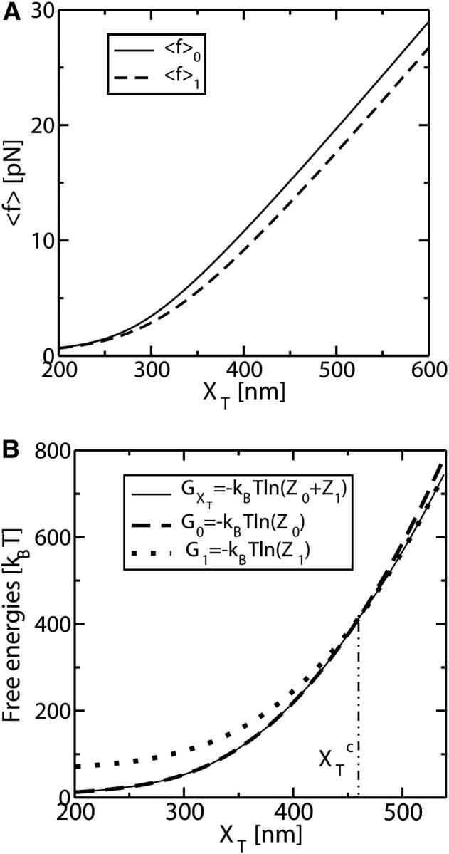
We consider a system with the parameters given in Tables 1 and 2. From the partition function analysis, we compute the following. (A) The two branches 〈f〉_σ, corresponding to the thermodynamic forces acting upon the system for a given σ RNA state as a function of X_T. (B) The free energy and the free energy of each branch σ, G_σ, as a function of X_T. Note that, upon increasing leaves the branch G₀ and enters the branch G₁ at . At the transition there is a jump in the slope of corresponding to a jump in the force 〈f〉 (Eq. 20).

The free energy of the system changes from one branch to the other at when both states are equally probable, ).

APPENDIX B: COMPUTATION OF THE FOLDING AND UNFOLDING RATES IN THE MIXED ENSEMBLE

We model the kinetics of the folding-unfolding of RNA as a Kramers' activated process characterized by the transitions rates

(B1)

where k₀ is an attempt frequency that depends on the shape of the free-energy landscape, on the molecular damping, and on the natural frequency of the hydrogen bond oscillations (Evans and Richie, 1997). The functions ΔG(X_T) and B(X_T) represent the difference of free energy between the F and UF states and the height of the kinetic barrier located between them (Fig. 2). (We stress that the physical meaning of ΔG(X_T) is completely different from ; see Eq. 15. The latter corresponds to the free-energy difference of the global system between two different values of X_T.) Using the results obtained from the partition function analysis, we can write ΔG(X_T) as

(B2)

where we used Eqs. 9–11. The parameter x_m is defined as the distance between the two states, x_m = 〈x〉₁ – 〈x〉₀; the functions W_r and ΔW_h are given by Eqs. 11 and 26.

The height of the barrier is given by the difference of free energy between the F state and the transition state, which we will denote as σ = t (averages taken when the molecule is in its transition state will be denoted by 〈…〉_t). The transition state is located at the point where the free-energy landscape of the system depicted in Fig. 1 is maximum (Fig. 2), and we define it as the RNA state where the first n* basepairs are opened and the latter N − n* are closed, N being the total number of basepairs that form the RNA molecule. Therefore the function B(X_T) is computed as the free-energy difference between the folded state and the transition state, which are separated by a distance x₁ = 〈x〉_t – 〈x〉₀,

(B3)

The function W_r is given by Eq. 11, and is the change in free energy of the handles when the RNA molecule jumps from the F state to the transition state, computed as

(B4)

The rates k_→, k_← associated to the activated process can be written as

(B5)

(B6)

with

(B7)

where we used Eqs. B1–B3. The expressions for the rates in Eqs. B5 and B6 are equivalent to those obtained by Bell (1978), but in the mixed ensemble. Note that the two rates k_→ (X_T), k_← (X_T) satisfy the detailed balance condition in Eq. 29 with ΔG(X_T) given by Eq. B2.

APPENDIX C: DEMONSTRATION OF THE EQUIVALENCE BETWEEN THE N_F AND N_R

The expressions for the fractions N_F and N_R are given by Eqs. 32 and 33. Integrating the dy′ term and using the initial conditions ρ_σ^F(R)(y, y) = 1, ∀σ, we get

(C1)

where y denotes a generic control parameter. We consider a symmetric perturbation protocol, Then, by using the evolution equation for the probabilities ρ_σ given by Eqs. 34 and 35, we obtain the relation

(C2)

where k_0→1 = k_→, and k_1→0 = k_←. Integrating by parts (Eq. C1) we get

(C3)

Finally, by using the relation between the probabilities ρ_σ for the forward and reverse process equation, we obtain

(C4)

References

- Bell, I. G. 1978. Models for the specific adhesion of cells to cells. Science. 200:618–627. [DOI] [PubMed] [Google Scholar]
- Bokinsky, G., D. Rueda, V. K. Misra, A. Gordus, M. M. Rhodes, H. P. Babcock, N. G. Walter, and X. Zhuang. 2003. Single-molecule transition-state analysis of RNA folding. Proc. Natl. Acad. Sci. USA. 100:9302–9307. [DOI] [PMC free article] [PubMed] [Google Scholar]
- Bolhuis, P. G., C. Dellago, P. L. Geissler, and D. Chandler. 2002. Transition path sampling: throwing ropes over dark mountain passes. Annu. Rev. Phys. Chem. 54:291–318. [DOI] [PubMed] [Google Scholar]
- Bouchiat, C., M. Wang, J. Allemand, T. Strick, S. Block, and V. Croquette. 1999. Estimating the persistence length of a worm-like chain molecule from force-extension measurements. Biophys. J. 76:409–413. [DOI] [PMC free article] [PubMed] [Google Scholar]
- Bustamante, C., J. F. Marko, E. D. Siggia, and S. Smith. 1994. Entropic elasticity of λ-phage DNA. Science. 265:1599–1600. [DOI] [PubMed] [Google Scholar]
- Bustamante, C., J. Macosko, and G. Wuite. 2000. Grabbing the cat by the tail: manipulating molecules one by one. Nat. Rev. Mol. Cell Biol. 1:130–136. [DOI] [PubMed] [Google Scholar]
- Cluzel, P., A. Lebrun, C. Heller, R. Lavery, J. L. Viovy, D. Chatenay, and F. Caron. 1996. DNA: an extensible molecule. Science. 271:792–794. [DOI] [PubMed] [Google Scholar]
- Cocco, S., R. Monasson, and J. Marko. 2003. Slow nucleic acid unzipping from sequence-defined barriers. Eur. Phys. J. E. 10:153–161. [DOI] [PubMed] [Google Scholar]
- Doudna, J. A., and T. R. Cech. 2002. The chemical repertoire of natural ribozymes. Nature. 418:222–228. [DOI] [PubMed] [Google Scholar]
- Essevaz-Roulet, B., U. Bockelmann, and F. Heslot. 1997. Mechanical separation of the complementary strands of DNA. Proc. Natl. Acad. Sci. USA. 94:11935–11940. [DOI] [PMC free article] [PubMed] [Google Scholar]
- Evans, E., and K. Richie. 1997. Dynamic strength of molecular adhesion bonds. Biophys. J. 72:1541–1555. [DOI] [PMC free article] [PubMed] [Google Scholar]
- Evans, E., and K. Richie. 1999. Strength of a weak bond connecting flexible polymer chains. Biophys. J. 76:2439–2447. [DOI] [PMC free article] [PubMed] [Google Scholar]
- Fang, X. W., P. Thiyagarajan, T. R. Sosnick, and T. Pan. 2002. The rate-limiting step in the folding of a large ribozyme without kinetic traps. Proc. Natl. Acad. Sci. USA. 99:8518–8523. [DOI] [PMC free article] [PubMed] [Google Scholar]
- Fernandez, J. M., S. Chu, and A. F. Oberhauser. 2001. Pulling on hair(pins). Science. 292:653–654. [DOI] [PubMed] [Google Scholar]
- Gerland, U., R. Bundschuh, and T. Hwa. 2001. Force-induced denaturation of RNA. Biophys. J. 81:1324–1332. [DOI] [PMC free article] [PubMed] [Google Scholar]
- Gerland, U., R. Bundschuh, and T. Hwa. 2003. Mechanically probing the folding pathway of single RNA molecules. Biophys. J. 84:2831–2840. [DOI] [PMC free article] [PubMed] [Google Scholar]
- Harlepp, S., T. Marchal, J. Robert, J.-F. Léger, A. Xayaphoummine, H. Isambert, and D. Chatenay. 2003. Probing complex RNA structures by mechanical force. Eur. Phys. J. E. 12:605–615. [DOI] [PubMed] [Google Scholar]
- Hummer G., and A. Szabo. 2003. Kinetics from nonequilibrium single-molecule pulling experiments. Biophys. J. 85:5–15. [DOI] [PMC free article] [PubMed] [Google Scholar]
- Imparato, A., and L. Peliti. 2004. Kinetic barriers in RNA unzipping. Eur. Phys. J. B. 39:357–363. [Google Scholar]
- Keller, D., D. Swigon, and C. Bustamante. 2003. Relating single-molecule measurements to thermodynamics. Biophys. J. 84:733–738. [DOI] [PMC free article] [PubMed] [Google Scholar]
- Liphardt, D., B. Onoa, S. Smith, I. Tinoco, and C. Bustamante. 2001. Reversible unfolding of single RNA molecules by mechanical force. Science. 292:733–737. [DOI] [PubMed] [Google Scholar]
- Liphardt, J., S. Dumont, S. B. Smith, I. Tinoco, Jr., and C. Bustamante. 2002. Equilibrium information from nonequilibrium measurements in an experimental test of Jarzynski's equality. Science. 296:1832–1835. [DOI] [PubMed] [Google Scholar]
- Marinari, E., A. Pagnani, and F. Ricci-Tersenghi. 2002. Zero-temperature properties of RNA secondary structures. Phys. Rev. E. 65:041919. [DOI] [PubMed] [Google Scholar]
- Moore, P. B., and T. A. Steitz. 2002. The involvement of RNA in ribosome function. Nature. 418:229–235. [DOI] [PubMed] [Google Scholar]
- Muñoz, V., P. A. Thompson, J. Hofrichter, and W. A. Eaton. 1997. Folding dynamics and mechanism of β-hairpin formation. Nature. 390:196–199. [DOI] [PubMed] [Google Scholar]
- Onoa, B., D. Dumont, J. Liphardt, S. Smith, I. Tinoco, and C. Bustamante. 2003. Identifying kinetic barriers to mechanical unfolding of the T. thermophila ribozyme. Science. 299:1892–1895. [DOI] [PMC free article] [PubMed] [Google Scholar]
- Ritort, F., C. Bustamante, and I. Tinoco. 2002. A two-state kinetic model for the unfolding of single molecules by mechanical force. Proc. Natl. Acad. Sci. USA. 99:13544–13548. [DOI] [PMC free article] [PubMed] [Google Scholar]
- Ritort, F. 2003. Work fluctuations, transient violations of the second law and free energy recovery in single molecule experiments. Poincaré Seminar. 2:193–226. Preprint arXiv:cond-mat/0401311. [Google Scholar]
- Russell, R., X. W. Zhuang, H. P. Babcock, I. S. Millet, S. Doniach, S. Chu, and D. Herschlag. 2002a. Exploring the folding landscape of a structured RNA. Proc. Natl. Acad. Sci. USA. 99:155–160. [DOI] [PMC free article] [PubMed] [Google Scholar]
- Russell, R., I. Millet, M. Tate, L. Kwok, B. Nakatani, S. Gruner, S. Mochrie, V. Pande, S. Doniach, D. Herschlag, and L. Pollak. 2002b. Rapid compaction during RNA folding. Proc. Natl. Acad. Sci. USA. 99:4266–4271. [DOI] [PMC free article] [PubMed] [Google Scholar]
- Smith, S., L. Finzi, and C. Bustamante. 1992. Direct mechanical measurements of the elasticity of single DNA molecules using magnetic beads. Science. 258:1122–1126. [DOI] [PubMed] [Google Scholar]
- Smith, S., Y. Cui, and C. Bustamante. 1996. The elastic response of individual double-stranded and single-stranded DNA molecules. Science. 271:795–799. [DOI] [PubMed] [Google Scholar]
- Smith, S., Y. Cui, and C. Bustamante. 2003. Optical-trap force transducer that operates by direct measurement of light momentum. Methods Enzymol. 361:134–162. [DOI] [PubMed] [Google Scholar]
- Tinoco, I., and C. Bustamante. 2002. The effect of force on thermodynamics and kinetics of single molecule reactions. Biophys. Chem. 102:513–533. [DOI] [PubMed] [Google Scholar]
- Zarrinkar, P., and J. Williamson. 1994. Kinetic intermediates in RNA folding. Science. 265:918–923. [DOI] [PubMed] [Google Scholar]
- Zhuang, X. W., T. Ha, H. D. Kim, T. Centner, S. Labeit, and S. Chu. 2000a. Fluorescence quenching: a tool for single-molecule protein-folding study. Proc. Natl. Acad. Sci. USA. 97:14241–14244. [DOI] [PMC free article] [PubMed] [Google Scholar]
- Zhuang, X. W., L. E. Bartley, H. P. Babcock, R. Russell, T. J. Ha, D. Herschlag, and S. Chu. 2000b. A single-molecule study of RNA catalysis and folding. Science. 288:2048–2051. [DOI] [PubMed] [Google Scholar]
- Zhuang, X. W., H. Kim, M. J. B. Pereira, H. P. Babcock, N. G. Walter, and S. Chu. 2002. Correlating structural dynamics and function in single ribozyme molecules. Science. 296:1473–1476. [DOI] [PubMed] [Google Scholar]