Coupling Field Theory with Continuum Mechanics: A Simulation of Domain Formation in Giant Unilamellar Vesicles

Abstract

Domain formation is modeled on the surface of giant unilamellar vesicles using a Landau field theory model for phase coexistence coupled to elastic deformation mechanics (e.g., membrane curvature). Smooth particle applied mechanics, a form of smoothed particle continuum mechanics, is used to solve either the time-dependent Landau-Ginzburg or Cahn-Hilliard free-energy models for the composition dynamics. At the same time, the underlying elastic membrane is modeled using smooth particle applied mechanics, resulting in a unified computational scheme capable of treating the response of the composition fields to arbitrary deformations of the vesicle and vice versa. The results indicate that curvature coupling, along with the field theory model for composition free energy, gives domain formations that are correlated with surface defects on the vesicle. In the case that external deformations are included, the domain structures are seen to respond to such deformations. The present simulation capability provides a significant step forward toward the simulation of realistic cellular membrane processes.

INTRODUCTION

Recent experimental evidence has shown the existence of fluid-fluid phase coexistence in the form of dramatic domain structures in giant unilamellar vesicles (GUVs) (Baumgart et al., 2004; Veatch and Keller, 2002, 2003; Veatch et al., 2004). In the case where ternary mixtures are considered, composed of cholesterol, sphingomyelin, and dioleoylphosphatidylcholine (DOPC) (Baumgart et al., 2004), cholesterol, dilauroyl phosphatidylcholine (DLPC), and dipalmitoyl phosphatidylcholine (DPPC) (Korlach et al., 1999; Feigenson and Buboltz, 2001), or cholesterol/DOPC/DPPC (Veatch and Keller, 2002, 2003; Veatch et al., 2004), the resulting fluid-fluid domains exhibit clear structure. The correlation with global curvature seems to be weak, and it is believed that line tension is more likely the key player in determining the domain sizes and shapes (Baumgart et al., 2004). Furthermore, in some cases, the domains are accompanied by distinct deformations on the vesicle surface, often in the form of circular bulges (Baumgart et al., 2004; Veatch and Keller, 2003). On the other hand, gel-liquid crystal domain coexistence has been observed in DPPE/DPPC mixtures (Bagatolli and Gratton, 2000), where, qualitatively, the shape of the domain is not highly correlated to the shape, or curvature, of the vesicle. Rather, the gel DPPE domains appear to be more painted on the surface of the vesicle. DPPC/DLPC gel-liquid crystal domains also seem to exhibit this behavior (Feigenson and Buboltz, 2001; Korlach et al., 1999), where the inclusion of cholesterol eventually results in solubilization of DPPC into the fluid phase, until the entire vesicle consists of only one fluid phase.

Domain formation on vesicles has also been examined theoretically (Seifert, 1993; Julicher and Lipowsky, 1993; Taniguchi, 1996; Jiang et al., 2000). Depending on whether the theoretical model is based explicitly on line tension (Julicher and Lipowsky, 1993) or composition (Taniguchi, 1996; Jiang et al., 2000; McWhirter et al., 2004), different results are predicted. Models based on line tension require that the system be pre-phase-separated into well-defined domains. From there, this particular free-energy framework can predict whether or not bulging or budding will form. The budding, or at least bulging, deformation is found from minimizing the free-energy subject to bending energy, line tension, and the constraint that the area of the domain is constant. Conversely, in the case that the free-energy model is based on composition, for example a Landau model for phase coexistence (Jiang et al., 2000; Van, 2002), then the model has the capability of predicting whether or not domains will form subject to the geometrical constraints of the problem. In this framework, domain formation can be further extended to include composition-curvature coupling, where the local curvature can perturb domain formation, along with curvature-composition coupling, where the local composition can then alter the local membrane structure. In the case where the latter type of coupling is restricted to variations in the membrane's material properties (i.e., in terms of a composition-dependent bulk and bending modulus), the result is soft and stiff regions on the membrane surface, depending on the location of the domains. This scenario has been examined in mesoscopic regimes (McWhirter et al., 2004) where the effects of thermal undulations were also considered. The drawback of employing a Landau model for composition is that, without additional coupling terms, it cannot directly influence the structure of the underlying membrane. In other words, it can predict whether or not domains will form, but once the domains have annealed, it cannot predict whether or not budding, or bulging, will occur. This fact is a simple consequence that the Landau model for composition, as it stands, will not result in specific composition-dependent stresses acting on the membrane.

Interestingly, real systems seem to exhibit behavior that is spanned by both theoretical frameworks: sometimes the formation of a domain is accompanied by an obvious shape change of the vesicle (for example, a bulge), and sometimes it is not. Thus, at the moment, two apparently different theoretical frameworks are required to model domain formation on vesicles. First, one model is required to predict whether domains will form, and then a second model is required to predict whether or not the resultant domains will alter the vesicle shape.

Regardless of the specific theoretical framework, a key limitation of these types of theoretical approaches is the evaluation of the actual free-energy functional itself. In the case of a Landau model for composition, only in relatively simple geometries can analytic solutions for the free-energy minima be found (Jiang et al., 2000), which is problematic if the GUV undergoes deformations. As such, the predictive power of these theoretical frameworks can be severely limited by the imposed geometrical constraints. If some means of efficiently evaluating these free-energy functionals in a completely unrestricted geometry could be found, then it may be possible to examine how domains form and couple to the shape of the underlying vesicle.

A tempting route of action is to model the formation of domains on GUVs employing molecular dynamics (MD) simulation, as this would, in principle, be able to distinguish, and perhaps even validate, the form of the ideal free-energy model framework by which to describe domain formation. However, examining domain formation on GUVs from MD is presently impossible as the lengthscales of GUVs are typically in the range of 20 μm, with a rough estimate of ∼10⁹ lipids constituting the vesicle. As such, even with coarse-grained MD methods (Marrink et al., 2004; Shelley et al., 2001; Rudd and Broughton, 1998; Kumar and Rao, 1998; Kumar et al., 2001; Laradji and Kumar, 2004), systems such as these are far beyond attainable simulation system sizes. Furthermore, the timescales, on the order of up to seconds, simply cannot be reached with present computational power and algorithms.

Another option is to employ continuum-level mechanics, where at least the underlying membrane dynamics, in the absence of composition field dynamics, can be examined using continuum-level modeling methods such as the material point method (Ayton et al., 2002b; York et al., 1999). However, once again, geometrical constraints are still a problem, which arise because of the grid-based framework employed in many continuum-level algorithms. In the material point method, the grid is used as a computational scratch-pad to evaluate continuum-level strains and strain-rates, and can be visualized as a three-dimensional lattice of points spanning the accessible space of interest. When thin structures like membranes are embedded within the grid, the transformation of in-plane quantities like the plane stress and strain to the grid can break down. As such, this type of scheme primarily works when the grid is actually bound in the plane of the membrane (Ayton et al., 2002b). Still, even though some computational problems exist with modeling membranes at the continuum level, the governing constitutive relation for membranes has been well studied (Hallet et al., 1993; Needham and Nunn, 1990; Rawicz et al., 2000; Olbrich et al., 2000), and, in the case of small deformations, it employs an elastic bulk modulus and a viscous shear viscosity (Evans and Needham, 1987; Ayton et al., 2002a). This combination of an elastic (solidlike) material property and a viscous (fluidlike) component is crucial for the membrane to perform all of its key functions (e.g., ion transport, lipid diffusion, lysis, fusion). In the case of very simple deformations (for example, the swelling of a vesicle due to osmosis or small surface deformations), an elastic constitutive model can be used (Ayton et al., 2002b). However, with a simple continuum-level membrane model, incorporating domains is still very difficult. At best, different prespecified regions on the surface of the GUV can be given different material properties corresponding to different domains. These can include, for example, a composition-dependent bulk modulus, thickness, and density. However these domains are fixed on the surface of the vesicle and, as such, they cannot move, coalesce, or change shape.

Another significant problem is that, without additional effort, continuum-level models make no contact with the underlying molecular-level interactions that ultimately determine the details of both the shape and the properties associated with domain formation on GUVs. A multiscale framework is required where the atomistic spatial temporal regime is connected in some way to the continuum-level. At its most minimal level, the bridge can be accomplished when, for example, the material properties such as the bulk modulus vary depending on the local composition, where the exact dependence is determined from atomistic-level non-equilibrium molecular dynamics (NEMD) simulations (Evans and Morriss, 1990; Ayton et al., 2002a; Ayton and Voth, 2004). In the context of our previous multiscale work (Ayton et al., 2002a,b; Ayton and Voth, 2002, 2004) this approach offers a computational means of bridging microscopic representations of the system with other representations that operate in higher length- and timescales. In the case of vesicles under osmotic stress, the lack of high amplitude thermal undulations (Marrink and Mark, 2001) allows for a direct atomistic, to continuum, bridge (Ayton et al., 2002b).

A Landau model for composition (Taniguchi, 1996; Jiang et al., 2000; McWhirter et al., 2004) can be incorporated into a multiscale simulation scheme by coupling the composition dynamics to the underlying membrane dynamics. The basic idea is that the composition fields are coupled with local surface deformations, and then the resulting domains affect the underlying membrane structure. The degree of this coupling can be varied, but the result is that domains of varying composition are not fixed on the surface of the vesicle, but can instead move, reform, and change shape. In fact, the formation of buds (Lipowsky and Sackmann, 1995; Seifert, 1993; Julicher and Lipowsky, 1993) is a classic example of how domains can couple to the underlying membrane structure.

Formally, at the continuum-level, the domains are defined by regions of a specific composition denoted by a variable φ, whose dynamics, i.e., dφ/dt, can be governed by either the time-dependent Landau-Ginzburg (LG) (Metiu et al., 1976; Van, 2002) or the Cahn-Hilliard (CH) equation (Metiu et al., 1976; Langer, 1971; Cahn and Hilliard, 1958). To bridge the underlying continuum-level membrane dynamics with the composition dynamics, a careful examination of the couplings between the two must be carried out. In fact, this approach has already been developed in the case of a small patch of membrane in the x,y plane (McWhirter et al., 2004), where the lengthscales were such that a mesoscopic membrane model (Ayton and Voth, 2002) could be employed. The multiscale bridge was accomplished by employing key results as found in previous work (Ayton et al., 2002b), to parameterize the mesoscopic model (Ayton and Voth, 2002). The planar geometry of the system (with the addition of small thermal undulations) allowed for the composition dynamics to be resolved via a Fourier transform method, such that the domain dynamics could be essentially be projected onto the undulating membrane surface. However, beyond this non-overlap geometry (the so-called Monge representation; Lin and Brown, 2004; Ayton and Voth, 2002), this scheme becomes exceedingly difficult.

To summarize the preceding discussion, if domains are to be successfully modeled on GUVs and other complex membrane surfaces, a computationally tractable continuum-level scheme is required for both the underlying membrane dynamics and the composition dynamics, with full coupling between the two. Fortunately, there exist alternative grid-free continuum-level methodologies known as the smooth particle methods, in particular smoothed particle hydrodynamics (SPH) (Lucy, 1977; Monaghan, 1992; Ellero et al., 2002) and smooth particle applied mechanics (SPAM) (Kum et al., 1995; Hoover and Hoover, 2003; Hoover and Posch, 1996). These schemes avoid many difficulties associated with traditional continuum-level simulation methods. SPH was originally developed to examine large-scale continuum-dynamics problems (in fact, astrophysical scenarios) (Lucy, 1977) and efforts have been made with SPH to improve the accuracy and stability of the method (see, e.g., Bonet and Kulasegaram, 2002; Bonet et al., 2004). On the other hand, the development of SPAM has tended more toward smaller-scale hydrodynamics, and in fact makes an elegant link with molecular dynamics (Hoover and Hoover, 2003). The correction schemes that appear in the SPH method (Bonet and Kulasegaram, 2002; Bonet et al., 2004) (typically associated with improving the numerical accuracy) have generally not been incorporated.

With SPAM, a continuum object can be thought of as being partitioned into a number of separate subsystems, such that each subsystem can be described by a state of local thermodynamic equilibrium (Evans and Morriss, 1990). In the case of a GUV with a diameter of ∼20 μm, for example, the surface of the vesicle may be partitioned into a large number of smaller areas, where each area is still, in itself, a large system relative to atomistic scales. The concept underlying SPAM is to then formulate the required continuum-level conservation equations for this partitioned system so the result is essentially a set of interacting free-energy particles that possess not only mass, position, and velocity, but possibly various other properties, for example composition, gradients of composition, and chemical potential. In a Lagrangian scheme, the SPAM particles not only translate according to local momentum conservation, but they can exchange various properties between one another. In the case of composition dynamics (either LG or CH), the SPAM particles would exchange composition, according to the underlying free-energy functional that governs the system. As such, SPAM can be thought of as both a computationally efficient means to solve continuum-level equations and as a conceptually attractive framework in which to recast continuum-level problems. In fact, if carefully formulated, the entire problem of coupled domain and vesicle deformation dynamics can be recast in a SPAM representation, and this is the topic of the present article. In doing so, almost all of the issues associated with the evaluation of complex free-energy functionals and grid-based schemes are avoided. Of course, the SPAM particles do not represent molecules, or anything remotely close. In the case of a membrane, they are best thought of as thin discs of mass that can exchange properties based on an underlying free-energy functional. It should be noted that solvent is included implicitly in the present model (i.e., bilayer properties), but explicit solvents (e.g., hydrodynamic effects such as fluid flows) can be readily included since SPAM has its origins in SPH. The coupling of a SPAM vesicle to a viscous SPAM fluid is clearly possible.

This article will therefore define a methodology to examine domain formation on GUVs coupled to its elastic deformations. The computational methodology will employ either LG or CH dynamics to model the composition dynamics. A fairly generic Landau model for composition (Taniguchi, 1996; Jiang et al., 2000) will be utilized as the underlying choice for the free-energy functional, in order to examine the form of the domain structures that emerge when the free-energy model is allowed to explore and couple with the underlying membrane deformations. In this approach, the composition fields are allowed freely flow over the surface of the deforming membrane so that they can find a free-energy minimum commensurate with the evolving and coupled geometry of the system. The entire problem, both composition and membrane dynamics, is recast with SPAM, resulting in a unified continuum-level description of the GUV system that can also be linked, in a multiscale sense, to atomistic-level properties.

COMPOSITION IN BINARY AND TERNARY MIXTURES

For a system of two components labeled a and b, the composition variable φ is defined as

(1)

where ρ_a is the mass density of component a, i.e., ρ_a = m_a/δV, and m_a is the mass of component a that is found in the small volume δV. The case where δV is constant will be considered here. Likewise, the mass density for component b is ρ_b, and the obvious condition that ρ = ρ_a + ρ_b.

In the case where ∂ρ/∂t = 0, one can write

(2)

where dφ/dt is the Lagrangian time-derivative of the composition and u is the flow.

In the case where the system is a ternary mixture of components a, b, and c, which phase-separates into an effective binary mixture, a similar definition of composition can be derived. Considering a situation similar to what was observed in Veatch et al. (2004), two phases, α and β, are defined where the mass density of the α phase is given by and is the mass density of the a-component that exists in the α-phase and likewise for the components b and c. Furthermore, the total mass density of component a in the two effective phases is given by and likewise for components b and c. In a similar manner, the mass density in the β-phase is defined as The composition variable φ for this effective binary system is given by

(3)

Again, the total mass density is ρ = ρ_α + ρ_β, and in the case where ∂ρ/∂t = 0, one again arrives at Eq. 2.

A LANDAU MODEL FOR PHASE SEPARATION

A generic Landau model will be employed in the present work to describe phase separation in a binary mixture (Van, 2002; Taniguchi, 1996; Jiang et al., 2000; McWhirter et al., 2004),

(4)

where F_M corresponds to a Helfrich bending energy and local area dilation free-energy contribution (den Otter and Briels, 2003; Lin and Brown, 2004; Brown, 2003; Brannigan and Brown, 2004; McWhirter et al., 2004), given by

(5)

where k_c is the bending modulus, H is the mean curvature, h is the membrane thickness, λ is a local bulk modulus, and ε refers to the local plane strain. It should be noted that this functional is appropriate for liquid and possibly gel bilayer phases, but not for the solid phase. In Eq. 4, F_φ is the standard Landau model for phase separation (Taniguchi, 1996; Jiang et al., 2000; Van, 2002; McWhirter et al., 2004)

(6)

where ζ² gives the strength of the nonlocal gradient term. Since we will specifically be dealing with membranes, dr = dA where dA is a local area element on the membrane evaluated in the correct in-plane reference frame. In cases where the membrane surface has complex undulations, or is an enclosed surface, the evaluation of these integrals can be quite complex (Jiang et al., 2000; McWhirter et al., 2004). In fact, one of the limiting factors in applying such free-energy models for membranes is evaluating these integrals on complicated, and perhaps even time-dependent, surfaces (Jiang et al., 2000).

Returning to the free-energy model, here V(φ) is a simple double-well potential given by

(7)

where n > m (both are positive), and a and b are constants. This strictly local term drives the composition within some area element dA to one of the minima in the potential. Other, more complex, free-energy models can be employed (McWhirter et al., 2004).

The functional F_φ in Eq. 6 is in fact a free energy even though it is sometimes referred to as an effective Hamiltonian (McWhirter et al., 2004). To appreciate this distinction, one can consider a partition function Z for a microscopic system given by

(8)

where Γ = {r₁,r₂,r₃,…r_N,p₁,p₂,p₃,…p_N}, r_i is the position of atom or molecule i, p_i = mv_i is the corresponding momentum, and C equals (m/2πℏ²β)^3N/2. The atomistic-level Hamiltonian is given by and β = 1/(k_BT) where k_B is Boltzmann's constant and T is the thermodynamic temperature. We now imagine coarse-graining the spatial extent of the system into M cells centered at locations {R₁, R₂, R₃,…R_M}. Note that R₁, the location of the cell 1, is different from r₁, the location of particle 1.

The composition of one of the cells, for example cell i, as determined from the real microscopic system, is denoted by where only the molecules within cell i contribute the local coarse-grained value of the composition. One can integrate over all compositions in cell i such that

(9)

where the notation φ_i = φ(R_i) is employed here, and φ(R_i) is an integration variable. The partition function Z can be rewritten as

(10)

where 𝒟φ ↔ dφ₁dφ₂dφ₃…dφ_M. However, except for simple lattice and spin models, F_φ cannot be easily evaluated (Mazenko, 2003). In practice, one employs a model F_φ whose parameters are chosen to reproduce experimentally determined phase structures at a specified resolution of measurement, for example, the width of a interface between two phases. The perceived or measured width at the mesoscopic scale will be different from the true microscopic width due to thermally induced variations of the location of the true interface. The formal procedure above, although not easily performed for real systems, does illustrate that F_φ is a scale-dependent free-energy functional. That is, the values of the parameters that enter into the model F_φ will depend on the size of the cells centered about the positions R_i (i.e., the degree of coarse-graining). Importantly, the integral in the last line of Eq. 10 is performed over all composition fields; however, below a critical temperature, those composition fields that correspond to a phase-separated configuration will receive the largest Boltzmann weight, and so are dominant in the contribution to Z.

The nonlocal behavior of F_φ occurs through the gradient-dependent composition term (Van, 2002), and, roughly speaking, drives the system to a uniform state of composition. As such, this term will be denoted by F_mix. Likewise, the term that contains V(φ), since it favors phase separation, will be denoted as F_demix. Thus, in this Landau model the free-energy minimum is found from the balance between nonlocal mixing and local demixing contributions to the free energy.

The final term in Eq. 4, F_{φ, H}, couples the composition φ to the curvature H via

(11)

where, in contrast to previous theoretical studies (Taniguchi, 1996; Jiang et al., 2000), a quadratic curvature coupling is employed here which can be justified by including a linear composition dependence to the bending modulus, i.e., k(φ) = k_c + k_φφ, where k_c is the usual one-component bending modulus that enters into F_M (Sackmann, 1994; Marrink and Mark, 2001; Lindahl and Edholm, 2000; Ayton and Voth, 2002) and k_φ = Λ. No other assumptions were employed in determining the functional form of the curvature coupling. It should be noted that under spherical geometries the result is that the membrane has no incentive to bend in either direction (i.e., bulge in, or bulge out). This quadratic form is in contrast to the more tradition linear coupling (Taniguchi, 1996; Jiang et al., 2000), which can result in dents and bulges depending on the local value of the composition. With the linear coupling model, a region with a negative composition will favor dents (i.e., H > 0), whereas regions with positive composition will favor bulges (i.e., H < 0). Although this form of the coupling does indeed result in interesting phase behavior, the justification of the linear form must be traced back to atomistic-level phenomena (i.e., explaining in terms of lipid structure, asymmetry of the bilayer, etc., why the domain with negative composition prefers dents in the GUV surface rather than bulges). The same situation applies for the domain with positive composition. In the present model, curvature coupling simply arises from the fact that the domain with the smaller bending modulus will have a correspondingly smaller free-energy cost to supporting a certain square of the curvature. Thus, the domain with the larger bending modulus will favor regions of smaller curvature, regardless of the sign. This form of curvature coupling, when tied to the underlying elastic membrane dynamics, results in a positive feedback scenario where domains with a smaller bending modulus collate in regions of locally higher curvature. The material properties of the domain are now modulated, and in this case, the curvature can actually be enhanced due to the local softening of the membrane.

COMPOSITION DYNAMICS

In this section the time evolution of the composition dynamics will be discussed. Both the time-dependent Landau-Ginzburg (LG) equation, and Cahn-Hilliard dynamics (CH) will be employed.

Landau-Ginzburg dynamics

The LG dynamics (Van, 2002; Metiu et al., 1976; McWhirter et al., 2004) for the composition field, φ, is given by

(12)

where F[φ, H] = F_φ + F_{φ, H} is the free-energy functional and the phenomenological coefficient, Γ, is positive. Under LG dynamics, a system should eventually reach the free-energy minimum; however, the actual dynamics are best thought of as relaxational, and as such, rigorously determining Γ for a particular system can be difficult. This equation of motion will drive the chemical potential of the composition field, μ = δF/δφ, to a target μ*, which is the chemical potential of the environment. Once μ = μ* a state of equilibrium is achieved, and the dynamics stops; however, the mean composition, 〈φ〉, is not conserved under this dynamics.

To evaluate the functional derivative, δF[φ, H]/δφ, care must be taken when considering the gradient term in F_mix, since strictly speaking this gradient is constrained to be in the plane of the membrane. Thus, if the gradient were evaluated in an unconstrained fashion, the normal component could appear. When evaluated in the plane of the membrane, and with b = a, the free-energy functional derivative, δF[φH]/δφ, is given by

(13)

where the gradient, ∇, is the required in-plane gradient regardless of the local orientation of the membrane. Of course, if this functional derivative were to be evaluated in a lab-reference frame, then much more work would be required.

In the case that Λ is non-zero, the dynamics must be constrained to conserve composition. Thus, in a Lagrangian form the constrained LG equation of motion can be written as

(14)

where α constrains the total composition of the system to be constant. This composition-stat, α, is related to μ* via 〈α(t)〉 = − Γμ*. The means by which such a constraint can be implemented will be discussed later.

The next step in the dynamical evaluation is to simplify the number of free parameters (i.e., Γ, ζ², a, and Λ). One option is to define a new set of scaled parameters as

(15)

where now all the strengths of the different components are expressed relative to the mixing term strength. This new parameter set is not unique, but it manages to factor at least one set of parameters (i.e., ζ²) into the LG prefactor, Γ. In the case that a dynamical simulation methodology is employed (as will be described later), the prefactor Γ* is essentially combined with the fundamental timestep of the simulation. A value of Γ* = 2 μm²/μs, combined with the timestep δt (as given in Table 1), resulted in stable dynamics in the present application. Much larger values of Γ*, for the given value of δt, resulted in the total composition not being conserved (even in the presence of the composition-stat). We note that the fundamental timestep δt was selected based on the underlying membrane dynamics.

TABLE 1.

Key parameters for the SPAM vesicle simulation

Parameter	Symbol	Value
SPAM cutoff	σ (10−6m)	1
Timestep	δt (μs)	0.0001
LG parameter	Γ* (μm2/μs)	2
CH parameter	M* (μm4/μs)	20
Unit of mass	m (10−16 kg)	ρAh/N
Modulus	λ0 (10−3 kg/(ms2)	5.4
Bulk modulus parameter	ɛ	10 to 100
Membrane thickness	h (μm)	0.0034
Relative demixing strength	a* (μm−2)	0.4 (rough); 0.2 (smooth)
Relative curvature coupling	Λ*	5 (rough); 8 (smooth)

The terms rough and smooth refer to the texture of the two SPAM GUVs examined.

Cahn-Hilliard dynamics

Cahn-Hilliard dynamics (Metiu et al., 1976; Langer, 1971; Cahn and Hilliard, 1958; McWhirter et al., 2004) conserve composition, but allow the chemical potential to fluctuate (McWhirter et al., 2004). In this case, Eq. 2 is expressed as

(16)

where the functional derivative was previously defined in Eq. 13. The final expression for the composition dynamics can be expressed in terms of a similar set of relative strength parameters as

(17)

where M* = Mζ²/2 and b* = a*. In this case, no constraint on the composition is required. In an analogous fashion to the value of Γ* in the case of LG dynamics, the value of M* that is chosen depends on the timestep. In this case, a value of M* = 20 μm⁴/μs, when combined with δt as in Table 1, resulted in conserved composition dynamics. Smaller values of M* could, of course, be employed. To relate M* to the real-time phase dynamics of the system, more atomistic-level information, either from atomistic-level MD simulation, or from experimental measurements, is required. This will be the topic of a future publication.

It should be noted that in McWhirter et al. (2004) a significant effort was made to parameterize the model to a known system (Ayton et al., 2002b). In the present study, such a detailed parameterization will not be made, as here we are interested in more generic phase behavior. However, in the spirit of a multiscale methodology, effort will be made to assign reasonable values to specific parameters (i.e., bulk moduli, curvature coupling strengths). Also, since the lengthscales for this system are on the order of micrometers, the coupling between thermal undulations and composition do not come into play, as any thermal undulation modes are subvisible, and thereby effectively renormalize the material properties.

The two previous dynamical schemes (LG and CH) are designed to take the system to the free-energy minima. However, it is possible to include noise fluctuations into the framework such that a dissipative dynamics results (Chaikin and Lubensky, 1995). Incorporating this thermal effect would allow the system to explore the free-energy minimum landscape via an additional stochastic noise source, ζ(r, t) added to Eq. 14 (LG) or Eq. 17 (CH), where the strength (magnitude) of the noise is such that fluctuation-dissipation is satisfied. For example, in the case of LG dynamics,

(18)

whereas, in the case of CH dynamics,

(19)

In the case of CH dynamics, the ∇² implies that a spatial correlation in the random noise is required for 〈ζ(r, t)ζ(r′, t′)〉 to be non-zero. In either case, to ensure that fluctuation-dissipation is satisfied, 〈ζ(r, t)ζ(r′, t′)〉 must be proportional to k_BT. In the present work, where the fundamental units of mass, distance, and time are as given in Table 1, at 308 K, k_BT ∼ 4.3 × 10⁻⁵ (10⁻¹⁶ kg(μm/μs)²), thus the noise term, if included, would have to be very small. However, incorporating this thermal effect into the dynamics will be explored in the future.

SMOOTH PARTICLE APPLIED MECHANICS (SPAM)

The previously described free-energy model (A Landau Model for Phase Separation), along with the two composition dynamics approach (LG and CH dynamics), still require a scheme in which to evaluate both the integrals that appear in the free-energy functional (Eq. 4), as well as the resulting equations of motion, Eqs. 14 and 16. Furthermore, the underlying membrane surface must be allowed to deform, and it cannot be restricted in terms of its topology. As discussed in the Introduction, smooth particle applied mechanics (SPAM) will be employed to resolve all dynamics. SPAM, which is very similar to smoothed particle hydrodynamics (SPH) (Monaghan, 1992; Ellero et al., 2002), is a Lagrangian formulation of fluid mechanics that employs smooth particles to represent continuum field variables (Lucy, 1977; Monaghan, 1992; Kum et al., 1995; Hoover and Hoover, 2003; Hoover and Posch, 1996). A interpolation scheme employing a short-ranged weight function W, with range given by σ, is used to define the continuum mass distribution. Here, the mass density at some position r, is given by

(20)

where the sum over j corresponds to the sum over all N SPAM particles. Following the notation in Hoover and Hoover (2003), the smooth particle mass evaluated at position r_i is expressed as

(21)

The Lucy Function (Kum et al., 1995) will be employed for W, given by

(22)

where σ is the lengthscale of the interaction, r = |r_i – r_j|, and D is a constant that normalizes W(r). In the case of a bilayer at macroscopic lengthscales, we consider a very thin membrane embedded in a three-dimensional volume. In this case, the normalization condition is expressed as 〈ρ(r)〉 = ρ₀, where ρ(r) is the (non-zero) mass density of the membrane at some position r and ρ₀ is the mass density of the membrane of interest. With this scenario, the continuum-level equations of motion are recast as motion equations for smooth particles, where the interpolated SPAM solutions converge to the exact continuum solutions by taking the correct limits (i.e., when N, the number of SPAM particles, becomes large and σ, the interpolation lengthscale, becomes very small). Details concerning the implementation of SPAM for viscous fluids can be found elsewhere (Kum et al., 1995; Hoover and Hoover, 2003; Hoover and Posch, 1996). Here, the focus will be on the application of SPAM to model elastic membranes coupled to composition dynamics.

Elastic membrane SPAM

Here a scenario considered where the underlying membrane, which in a sense forms the computational grid for the composition dynamics, is allowed to deform in time. Furthermore, the focus is on closed surfaces, i.e., vesicles (although this is not a requirement). Thus, the first task is to apply SPAM to the problem of membrane dynamics, where the possibility of introducing external perturbations is allowed; for example, poking the membrane with an external probe, much as is done in micromanipulation experiments (Rawicz et al., 2000; Olbrich et al., 2000). More complex deformations are, of course, possible, but they will not be explored here.

The solution to the momentum conservation equation is required, which is written as

(23)

where P is the stress tensor, n is the number density, F is an external force, ρ is the mass density, and a is the acceleration. To solve this equation, a constitutive relation is required, where an elastic constitutive relation for the plane stress is employed here (Ayton et al., 2002a,b), given by

(24)

where ΔA = A − A₀ and A₀ is the initial area. In this expression, a local coordinate frame is defined where the membrane normal is along the local z axis, and thus the x and y axes are orthogonal and in the plane of the membrane. In the case of a perfectly spherical vesicle for example, the local z axis would lie along the radial vector of the vesicle. Likewise P corresponds to the negative of the plane stress. The bulk modulus is given by λ, and it can be calculated from atomistic non-equilibrium molecular dynamics (NEMD) simulations for specific systems (Ayton et al., 2002a,b).

In some cases, the bulk modulus can have a significant composition dependence (Ayton et al., 2002b). The composition was thus coupled to the underlying elastic membrane via

(25)

where λ_φ = λ₀/ɛ, λ₀ is as given in Table 1, and ɛ is a constant that determines the strength of the composition-dependent perturbation. The linear composition dependence on the bulk modulus mirrors the composition dependence of the bending modulus, which is responsible for the composition-curvature coupling term in the free-energy functional, Eq. 11. Higher order terms in Eq. 25, e.g., terms involving |∇φ|², could also be included. Values of ɛ range from 10 to 100, depending on the strength desired, and the actual value of λ₀ was selected from that previously found from NEMD simulations of DMPC/cholesterol mixtures (Ayton et al., 2002b) and taken to correspond to a 1:1 mixture of DMPC/cholesterol. Of course, in this study the possibility is left open that the two phases might actually correspond to a ternary mixture that has phase-separated into an effective binary mixture. However, this intermediate value of λ₀ is a reasonable estimate. To get a more exact value of λ₀, a series of NEMD simulations as in Ayton et al. (2002a,b), corresponding to the explicit system under study, would need to be performed. Given that the bulk modulus is proportional to the bending modulus (Lipowsky and Sackmann, 1995; Brannigan and Brown, 2004), it is reasonable to assume that this relationship carries over to the bulk modulus. The result of this composition-dependent bulk modulus is that regions of φ ∼ −1 become softer, whereas regions with φ ∼ 1 become stiffer and resist stretching.

With SPAM, momentum conservation, Eq. 23, is expressed as Kum et al. (1995), Hoover and Hoover (2003), and Hoover and Posch (1996),

(26)

where ρ_i = ρ(r_i) and W(|r_i−r_j|) is an appropriately normalized smooth weight function (Kum et al., 1995; Hoover and Hoover, 2003). If Eq. 24 is substituted into Eq. 26, one obtains

(27)

where λ_j and λ_i incorporate the composition dependence of the bulk modulus for different SPAM particles. The ratio (A/A₀)_i can also be calculated with SPAM via changes in the density as

(28)

where ρ_i0, for example, corresponds to the initial mass density of SPAM particle i, and in general ρ_i0 ≠ ρ_j0 for i ≠ j.

Thus, in the case that the initial starting structure is a well-defined membrane, the equation of motion in Eq. 27 will automatically evaluate the required in-plane stress response. In this way, SPAM has yielded an easily evaluated elastic membrane model. It is important to note that generally the separation of in-plane and out-of-plane stress components is not trivial in cases when the surface of the membrane has complex undulations. Finally, an additional dampening term can be included in Eq. 23 as was done in Ayton et al. (2002b). A test of the accuracy of SPAM for the membrane dynamics is given in the Supplementary Material.

Composition dynamics with SPAM

The SPAM-membrane scheme described in the previous section only solves the underlying membrane dynamics. To include, and couple, the composition dynamics (given by Eqs. 14 and 16) a similar SPAM decomposition for dφ/dt must also be performed.

Before proceeding, a brief review of the relevant SPAM (or SPH) methodology is in order. A more detailed discussion can be found in, for example, Kum et al. (1995), Hoover and Hoover (2003), and Hoover and Posch (1996). The discussion here will be restricted to the problem of representing composition, φ, and any associated gradients, with the SPAM methodology.

With SPAM, the continuum value of the composition, φ(r), can be expressed through

(29)

where φ_j is the composition of SPAM particle j. Thus a SPAM particle can carry with it the intrinsic particle property of composition. If the previous expression is evaluated at location r_i, that is, the instantaneous location of SPAM particle i, one obtains

(30)

Note that the continuum value of the composition at r_i, φ(r_i), is not necessarily the same as the particle property φ_i (but, computationally, they are found to be very close). More importantly, gradients of composition at r_i can be evaluated via

(31)

where (∇φρ)_i is evaluated at r_i, and the notation ∇_i = d/dr_i has been employed. Since W is only a function of r_ij = |r_i−r_j|, one can write

(32)

In subsequent equations, the compact notations ∇_iW(|r_i − r_j|) = ∇_iW_ij and ∇_jW(|r_i − r_j|) = −∇_iW_ij will be employed. Considering that

(33)

one can evaluate (∇φ)_i as

(34)

where ρ_ij = (1/2)(ρ_i + ρ_j). Employing the symmetric version of the density ensures that, at a pairwise level (i.e., considering two isolated SPAM particles labeled i and j), (∇φ)_i = (∇φ)_j. This feature of SPAM, that being an enforced pairwise symmetry, carries over to more complex scenarios; for example when curvatures of various quantities are considered.

Again, employing φ as an example particle property, one can also employ SPAM to evaluate ∇²φ. Any scalar particle property can be used, for example the chemical potential, μ (as would be required under CH dynamics). For a composition field whose free energy is given by F_mix, the LG dynamics requires ∇²φ,

(35)

where the second line results from the functional derivative of F_mix with respect to composition. To evaluate ∇²φ with SPAM, ∇²φ can be rewritten as

(36)

where χ is equal to ∇φ. One then has

(37)

If a SPAM decomposition along the lines of that employed to solve Eq. 23 is employed, an equation for the gradient of χ can be written as

(38)

where the additional particle property χ_i has been introduced. The form of Eq. 38 is similar to the SPAM equation for momentum conservation, Eq. 26.

In the case of CH dynamics, ∇²μ is required (i.e., Eq. 16), where μ = δF[φH]/δφ. Again, ∇²μ = ∇ · ζ where ζ = ∇μ. With SPAM, these expressions become

(39)

and

(40)

Thus, under CH dynamics, SPAM particles not only carry composition as an intrinsic particle property, but also as the chemical potential. More importantly, the SPAM particles can exchange these properties between one another.

In the case of LG dynamics, the final SPAM-LG equation of motion is given by

(41)

where α_i is found from an integral feedback mechanism similar in form to the more familiar Nosé-Hoover integral feedback (Hoover, 1985; Evans and Holian, 1985). In this expression, u_i is the velocity of SPAM particle i.

In the case of CH dynamics, a similar expression is found, given by

(42)

where, in this case, no constraint on the total composition is required. Again, μ_i = (δF[φ, H]/δφ)_i, where the notation (…)_i implies that the functional derivative is taken first, then the resulting expression is formulated with SPAM and evaluated at position r_i.

COMPOSITION DYNAMICS OF GUVS: STATIC MEMBRANE

A SPAM GUV was constructed where an initial set of SPAM particles, randomly placed on the surface of a sphere of radius 12.6 μm, were allowed to anneal via Eq. 26, subject to the constraint that the particles had to remain close to the surface of the sphere. The constraint was implemented by simply projecting out any accelerations and velocities parallel to the local GUV radial vector. For very small annealing timesteps, the SPAM particles were very closely bound to the ideal GUV surface, whereas for timesteps similar to that employed in Table 1, small deviations resulted. The annealing was performed by employing a symmetrized density (i.e., ρ = 0.5(ρ_i + ρ_j)) and with

(43)

where a = 5 μm⁵/(10⁻¹⁶ kg μs²) and I is the identity matrix. This initial form for P results in an MD-like repulsive pair potential between SPAM points (Hoover and Hoover, 2003), providing a convenient means of annealing particles into low energy configurations. The bulk moduli, λ_i, were all fixed at λ_i = λ₀. The tolerance for the constrained dynamics was set such that small dents and bulges in the vesicle surface could form, resulting in small local variations in curvature. After the annealing process, the locations of the SPAM particles were frozen, thus creating a static membrane surface. Once this initial annealing procedure was completed, the elastic SPAM membrane interaction (Eq. 27) was then employed. The SPAM membrane is held together by the pairwise elastic contributions as in Eq. 27. For example, in the case that a local region of the membrane is dilated from its initial state, the membrane will respond with a local acceleration that results in contraction. Likewise, if a local region is compressed, the membrane pushes back. Moreover, the direction of the resultant acceleration will closely follow the desired in-plane response.

Performing a SPAM simulation requires two key resolution parameters: the lengthscale of W, which is given by σ, and then the reduced density, written as

(44)

where the density has been explicitly defined in terms of the membrane of thickness h. At continuum lengthscales (i.e., units of μm), σ > > h. The lengthscale of W was set at σ = 1.0 μm and ρ* = 2. Other parameters are given in Table 1. It is important to note that at this lengthscale (i.e., μm) any thermal undulations are subvisible and are not resolved at the SPAM level. To be very clear, it is the nanometer scale thermally induced bending undulations (Evans and Rawicz, 1997; Rawicz et al., 2000) that are below the resolution of the model, and large-scale shape changes are indeed possible within this methodology. Here, the pre-prepared state of the GUV corresponds to one where the vesicle is under an osmotic stress. As such, the initial area, A₀, that is used in the constitutive relation for the membrane dynamics (Eq. 27) corresponds to a local area evaluated in the prestressed state. The membrane could be further dilated from this point using an effective osmotic stress using methods previously developed (Ayton et al., 2002b). As such, deformations in the underlying membrane surface must come from external sources or from static local variations in curvature.

The local curvature can be measured by first calculating ∇²ρ, the curvature of the membrane density, and then by defining H, the curvature, via H = Ω∇²ρ, where Ω is a constant with units of μm⁴/10⁻¹⁶ kg. The constant Ω can be easily estimated in the case of spherical vesicles by noting that

(45)

where the average is taken over the surface of the vesicle, r is the radius of the vesicle, and the factor of 2 comes from the fact that the surface is spherical.

Two SPAM GUVs were created: one with a rough surface, where the constraint tolerance was set to be low and the annealing process was terminated early, and one with a smooth surface, where the constraint tolerance was increased and a long annealing process was employed. By constructing two different underlying membrane surfaces, the correlations between domain formation and local curvature could be more fully examined. Moreover, it is important to note that the deviations in curvature are very small by design, as the goal in this study is to see how small deviations in local curvature can couple to domain structure. The rough vesicle contained a number of surface defects, whereas the smooth vesicle contained only very small surface deformations. In Fig. 1, the lowest set of two snapshots show how the small surface irregularities are distributed over the SPAM GUV surface. The more darkly shaded blue regions correspond to regions of more negative curvature, with the darkest regions denoting those regions of the largest negative curvature (i.e., a bulge). The white regions actually correspond to local regions of positive curvature (i.e., a dent).

FIGURE 1.

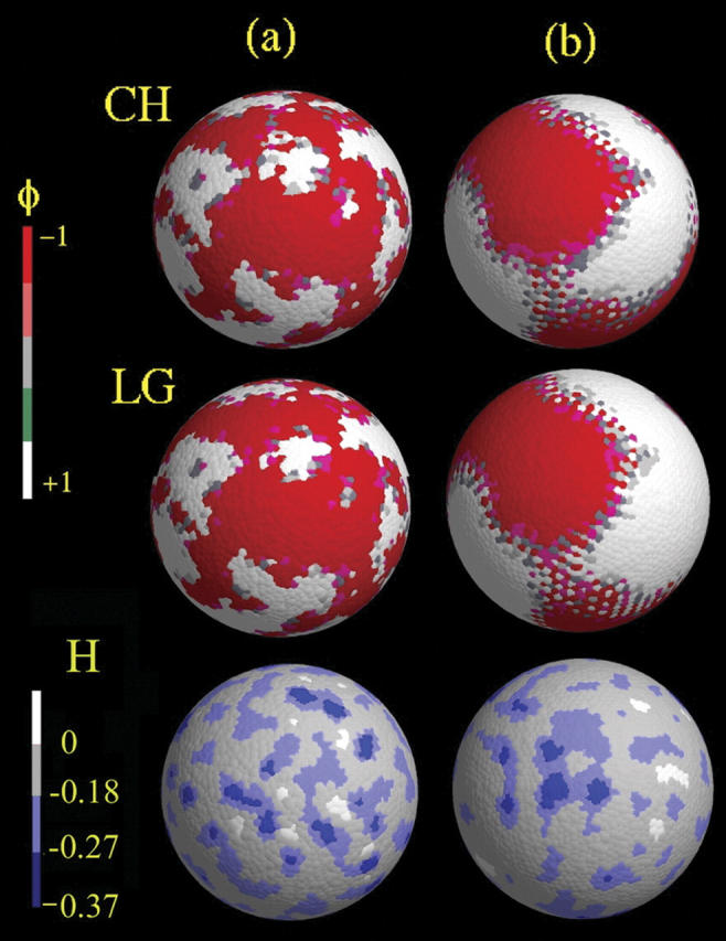
Column a, SPAM simulation snapshots of the rough GUV after 700 μs with a* = 0.4 μm⁻² and Λ* = 5. The top image corresponds to CH dynamics, whereas the middle employs LG. Column b, SPAM simulation snapshots of the smooth GUV with a* = 0.2 μm⁻² and Λ* = 8. The top image corresponds to CH dynamics, whereas the middle employs LG. The red regions correspond to domains with φ ∼ −1, whereas the white regions have φ ∼1. The corresponding curvature fields as found from H = Ω∇²ρ are shown on the bottom two images, where the color-coding scheme is given on the bar on the left. The dark blue regions correspond to dents, whereas the white regions correspond to bulges.

One can define an apparent GUV radius from Eq. 45 with Ω = 1 μm⁴/10⁻¹⁶ kg, which can be used as a diagnostic to define how accurately ∇²ρ is measuring the curvature. In the rough case of 〈H〉 = −0.186Ω, it is found that 〈∇²ρ〉 gives an apparent vesicle radius of 10.8 μm, which is slightly less than the actual radius of the vesicle, whereas, in the smooth case, the apparent radius was found to be ∼13.7 μm. In either case, enforcing that Ω = 1 μm⁴/10⁻¹⁶ kg, and measuring the curvature directly via the SPAM curvature of the density, is a reasonable approximation. It should noted that in measuring the curvature, a SPAM weight function with a larger cutoff was employed, where σ_c = 3σ and σ represent the original cutoff. This was found to be necessary to obtain a smoother local measure of the membrane curvature. In contrast to the composition dynamics where large gradients such as ∇φ occur, ∇²ρ is small and requires a slightly longer range to detect the mass density curvature.

The results for the static rough GUV will be presented here first. Both LG and CH dynamics were employed; however, it is important to note that the LG dynamics do not conserve composition when the curvature coupling term is included. As such, a composition-stat was employed (Eq. 41). However, even with the composition-stat, the LG dynamics seeks the minima, but not necessarily in a physically meaningful way. In fact, an inspection of Eq. 41 reveals that the LG dynamics with α_i can, in essence, pull composition out of the air or from a fictitious composition reservoir whose chemical potential is −〈α〉/Γ. That is, whereas the curvature coupling term will always drive the composition to more negative values, the composition-stat, α_i, adds positive composition to maintain the constraint that the composition must remain constant.

In contrast, the CH dynamics, by virtue that it changes composition via fluxes, cannot locally create or destroy composition. Rather, it must be transferred from one region to another in a conserved fashion. It is important to note that, although the total composition of the system is constrained to be constant (i.e., zero), there is nothing explicit in either the LG or CH dynamics, which constrains φ to be rigorously bounded by ±1. Thus, the bistable potential V*(φ) in Eqs. 7 and 15 acts not only to phase-separate the system but is also a potential barrier to keep the composition within ±1. As such, the potential was chosen to be V*(φ) = a*φ¹⁰/10 − b*φ²/2, which results in very steep repulsive walls, where, in all cases, b* = a*. The values chosen for a* and Λ* are listed in Table 1, and the simulations were performed over 300 μs. The values chosen for a* and Λ* are not unique, and very similar behavior was observed for a* ∼0.2 − 0.6 and Λ* ∼0.2 − 1.0. This behavior will be discussed in more detail in the next section.

The composition dynamics simulations were initialized by randomly assigning each SPAM particle a composition between 1 and −1, such that the total average composition of the system was zero. As the system evolved in time under either CH or LG dynamics, the initial composition distribution changed, eventually reaching a free-energy minimum.

The difference between CH and LG dynamics is more clearly seen if the free-energy time-evolution is examined. The free energy of the SPAM system can be evaluated from Eq. 4. Defining the average number density ρ_N = N/A, where A is the surface area of the GUV, and considering the case where local density fluctuations are small, then the free energy can be expressed as

(46)

In Fig. 2 a, the quantity 2F_T[φ,H]ρ_N/ζ² is shown for the smooth GUV, where the LG dynamics (solid lines) are characterized by an initial fast relaxation, while the CH dynamics (dashed lines) exhibits a roughly 1/tⁿ behavior. The origin of the fast LG free-energy decay is not immediately clear, but it suggests that after a relatively fast relaxation the system reaches a free-energy minimum. The CH dynamics, on the other hand, approaches the free-energy minimum in a slightly different fashion. The interesting point is that even though the raw LG dynamics do not conserve composition in the case that curvature coupling is included, they still seem to reach a similar free-energy minimum as the CH dynamics when the composition-stat is included. Apparently, the ad hoc addition of the composition-stat not only maintains constant total composition, but actually assists in directing the system to the free-energy minimum.

FIGURE 2.

The time-evolution of the scaled free energy, 2F[φ,H]ρ_N/ζ², under CH and LG dynamics for the smooth GUV. The pair of curves in a corresponds to the original smooth GUV with a* = 0.2 μm⁻² and Λ* = 8. The lower two pairs of curves correspond to systems undergoing the external deformation, resulting in two symmetric dents along the simulation x axis. The curves in b correspond to a* = 0.2 μm⁻², Λ* = 8, whereas c is a* = 0.2 μm⁻², Λ* = 4. In each case, the lower curve in the pair corresponds to the LG dynamics case (solid line), whereas the upper curve in the pair corresponds to the CH dynamics (dashed line).

That the two dynamics give similar free-energy minima can also be seen in Fig. 1, where the system has phase-separated into two phases with very similar domain structure (here the red regions correspond to domains with φ ∼ −1, whereas the white regions have φ ∼ 1). The locations of the domains are seeded by the small variations in the local curvature, as shown in Fig. 1 (lower pair of images); here the dark-blue regions corresponding to more negative curvature H are roughly correlated with the red domains seen in the upper panels of Fig. 1. These small bulges tend to anchor the domains spatially, inhibiting the system from reaching a completely phase-separated state (in the spherical GUV case, this would eventually correspond to the system separating into hemispherical domains). The rough GUV, as shown in Fig. 1 a (left column of images) shows a patchy domain structure under both CH and LG dynamics, whereas the smooth GUV in Fig. 1 b (right column of images) has a more organized structure.

COMPOSITION DYNAMICS OF GUVS: DYNAMIC MEMBRANE

In McWhirter et al. (2004) a scenario was considered where domain formation was examined at mesoscopic lengthscales, with thermal undulations giving significant deformations of the membrane. In contrast, the lengthscales employed in this study are much greater and on the order of μm, far beyond resolvable amplitudes of the thermally induced membrane undulations. As such, for the membrane to actually deform in time, some sort of external perturbation must be included.

One possibility for an external deformation would follow along the lines of micromanipulation experiments (Rawicz et al., 2000; Olbrich et al., 2000) where, in essence, the GUV is poked, resulting in an indentation. In situations where the domain formation was coupled to curvature, this experiment could give insight into the details of the coupling. Of course, in the case that curvature coupling is small, or even non-existent, then this external deformation should not perturb the underlying domain structure. Either way, this simple deformation results in a controlled means of introducing a locally enhanced region of curvature on the vesicle surface that could influence and even alter domain formation. It should be noted that an end goal of the present methodology development is to describe cellular interactions where such deformations are clearly important.

With the present SPAM LG/CH-membrane model, including a small external deformation and allowing the composition to couple can be readily implemented. Since the SPAM representation of the composition dynamics (as given by Eqs. 41 and 42) naturally resolves the problem in the required reference frame, incorporating external deformations requires no additional work. In fact, when membrane deformations are considered, the simplicity and elegance of the SPAM method becomes evident. As opposed to requiring the calculation of complex Jacobians and/or transformations, SPAM automatically evaluates the required quantities in the correct local reference frame, regardless of the local orientation of the membrane. Once the deformation is imposed on the GUV, the composition can then respond via the free-energy functional, Eq. 4.

The smooth GUV as described in the previous section, with its parameters given in Table 1, was subjected to a deformation in the form of an indentation along the simulation x axis, such that a small dent resulted on opposite ends of the vesicle. This symmetric deformation kept the total momentum of the GUV at zero. The shape of the dent was designed to mimic the shape of the tip of an external probe, which could be, for example, a narrow rod ∼5–10 μm in diameter, with a slightly rounded tip. The actual details of the structure of the probe are not crucial here; only the resulting force acting on the GUV was actually employed. As the tip was pushed in slightly over the course of 12 μs, the average radius of the GUV (defined as r_avg = 〈r_i〉, where r_i is the radius of the GUV evaluated at the location of SPAM particle i) decreased from ∼12.61 μm to ∼12.58 μm.

Then, under LG and CH dynamics, the composition was allowed to couple to this deformation over the course of 700 μs. The time evolution of the free energy is shown in Fig. 2, where the pair of curves in Fig. 2 b correspond to systems with a* = 0.2 μm⁻², Λ* = 8, whereas the pair in Fig. 2 c had a* = 0.2 μm⁻², Λ* = 4. In each pair, the lower curve corresponds to the LG dynamics case (solid line), whereas the upper curve corresponds to CH dynamics (dashed line). Clearly, including the dent has resulted in a substantially lower free energy relative to the undented case (Fig. 2 a), and even under fairly weak curvature coupling (i.e., the curves in Fig. 2 b) the system can access a lower free-energy state. Again, after a sufficiently long time, both the CH and LG dynamics converged to very similar structures.

When compared to how the radius of the GUV changes, the effect of the external deformation on the free energy persists over much longer times (even though it took only ∼12 μs for the dent to form). This effect is due to the slow reorganization of the domain structure in response to the indented surface.

A snapshot of the dented GUV is shown in the lower image of Fig. 3. The undented GUV with identical parameters, and in exactly the same orientation, is shown in the upper image. This snapshot is the same GUV as in Fig. 1 b, i.e., the smooth GUV, but with a different orientation. As was observed previously, the small surface irregularities (indicated here by blue regions corresponding to curvatures where H < −0.27 μm⁻¹), act as nucleating sites for negative composition, eventually anchoring φ ∼ −1 domains.

FIGURE 3.

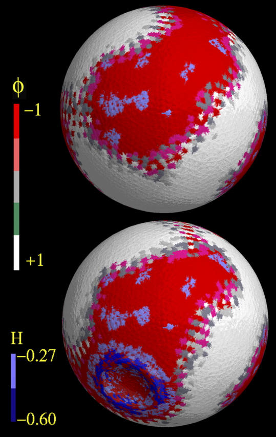
Dynamic composition coupling to induced curvature. The upper image is a snapshot of the smooth GUV as in Fig. 1 b, but rotated slightly. The lower image is the same system in exactly the same orientation, but with a dent located at the x-axis poles. Both snapshots were obtained after 700 μs with CH dynamics, with starting conditions as described in Composition Dynamics of GUVs: Static Membrane. The color-coding for the composition is given in the bar on the left of the image, where red corresponds to φ ∼ −1 and white corresponds to φ = +1. The blue regions are the local curvature field superimposed on the images.

With this level of SPAM resolution (N = 4000 SPAM particles), the domain boundaries are not perfectly sharp, as shown by the intermediate colors in the boundaries. At this level of resolution, only 50 h of CPU time, in serial, on a 1533-mHz AMD Athlon PC, was required. As such, resolutions an order-of-magnitude higher are within computational reach. In fact, using massively parallel schemes (Ayton and Voth, 2004), resolutions up to three orders-of-magnitude higher are possible. Likewise, at the present resolution, simulations three orders-of-magnitude longer in time are readily accessible.

The effect of denting the GUV is clearly evident. In the lower image of Fig. 3, the blue ring of large negative curvature, corresponding to the perimeter of the dent, is now embedded within a φ ∼ −1 domain that was not present in the undented case (upper image). The original φ ∼ −1 domain, as seen in the upper image, flowed out and enveloped the dented region. Also, new regions of φ ∼ +1 have formed near the top of the vesicle so as to maintain a total composition of zero. Thus the effect of the dent is not a strictly local phenomenon, and it can alter domain structures in other regions of the vesicle. These interesting results may also be pertinent to the formation and evolution of lipid domain rafts in real cellular membranes (see, e.g., Radhakrishnan et al., 2000; Pralle et al., 2000; Simons and Ikonen, 1997). This will be a topic of future studies in our group.

These results demonstrate that domain formation can, in a sense, be controlled by externally imposed deformations on vesicles. Of course, the degree of control is directly related to the degree of curvature coupling in the system. As such, this fairly simple test, whether carried out with a Landau free-energy model or with a real experiment, could indicate whether or not the curvature coupling is a key interaction in the system.

COMPARISON WITH EXPERIMENT

In Composition Dynamics of GUVs: Static Membrane, a static membrane was prepared with small surface deformations in the form of dents and bulges, and it was found that the resulting domain structures were highly influenced by small local deviations in curvature. The small dents and bulges acted like both nucleation sites and domain anchors inhibiting the domains from coalescing into larger structures. In the absence of the curvature-composition coupling, the coalescence would have eventually led to a complete phase separation.

The experimental fact that some vesicles appear to form bulged domains (Veatch and Keller, 2003; Baumgart et al., 2004), whereas some do not (Veatch and Keller, 2002, 2003; Bagatolli and Gratton, 2000), suggests that the full free-energy model should span the entire regime from composition (Taniguchi, 1996; Jiang et al., 2000) to line tension (Julicher and Lipowsky, 1993). The present model seems adequate to explain those cases where bulged domains do not appear. The present static membrane model can be thought of as an adiabatic case, where the composition dynamics can fully anneal to the underlying structure. Still, even when the underlying membrane is static, some interesting comparisons with experimental observations can be made. Firstly, the domain structures in Fig. 1, a and b, clearly look nothing like the dramatic bulged structures in Baumgart et al. (2004) and Veatch and Keller (2003), where circular domains bulge out of the vesicle. A least qualitatively, the present results appear more like the patchy gel-liquid crystal domains as found in Korlach et al. (1999) and Feigenson and Buboltz (2001) or in Bagatolli and Gratton (2000). Of course, in our simulations, the phase of the domain (i.e., liquid, gel, or even solid) cannot be distinguished. Still, as noted in Veatch and Keller (2002), liquid-liquid phase coexistence (typically observed at cholesterol concentrations of ∼10 mol % to 50 mol %) is characterized by circular domains that eventually coalesce into larger domains. However, when the phase coexistence is solid-liquid, the solid domains are not necessarily circular, and do not always merge.

Thus, based on these results, an interesting observation can be made. In the gel-liquid crystal domains (Korlach et al., 1999; Feigenson and Buboltz, 2001; Bagatolli and Gratton, 2000) it is reasonable to presume that the difference in the bending modulus in the gel- and liquid-crystal phases is fairly significant (compared to the fluid-fluid domains; Baumgart et al., 2004). Furthermore, the domains in these systems are not generally spherical and they do not coalesce. The domain structures observed in Fig. 1 a result from a free-energy model where the curvature coupling to composition arises from a composition-dependent bending modulus. At least qualitatively, the domain structures in the simulation are similar to those observed in experiment. Thus, in the experimental case, could it be possible that these domains have been both nucleated and anchored by very small, perhaps almost not-measurable, variations in local curvature?

The present free-energy model also employs a minimalist feedback in terms of how domains can alter the actual structure of the membrane. The model employed here can form domains, depending on the balance of mixing, demixing, and curvature coupling, but, once the domains have formed their effect on the underlying membrane, is limited to perturbing the elastic material properties that appear in the constitutive relation (Eq. 24). Thus, at best, the membrane will become softer (φ ∼ −1) or stiffer (φ ∼1) due to domain formation, but no new driving forces will be introduced that will cause the membrane to bulge or distort. This minimalist feedback to the underlying membrane structure could significantly restrict the system from further deforming. Our future work will seek to generalize this model.

In the case where a large dent is created by an external force, the original domain formation is drastically perturbed. Even regions far away from the dent can have altered domain structures. In this case, the induced curvature of the large dent attracts domains that are composed of the soft material (i.e., with a lower bulk and bending modulus). The subsequent softening of the material allows the external probe to push in a bit farther, thus increasing the curvature. It would be very interesting to see experimentally how real vesicles with domain structures respond to external deformations.

SUMMARY

Composition dynamics and domain formation have been examined in this article on GUVs by extending a novel continuum modeling scheme known as SPAM. A relatively generic Landau model for phase separation, extended to include curvature coupling via a linear dependence of the bending modulus, was coupled to an underlying elastic membrane model for the GUV. Both the time-dependent Landau-Ginzburg and Cahn-Hilliard dynamics were then used to solve the composition dynamics within an overall SPAM-like algorithm. It was found that recasting the entire problem with SPAM resulted not only in much simpler expressions than those obtained by more standard means, but also that the resulting simulation method was both efficient and surprisingly accurate, given its relative simplicity.

The preliminary goal of this work was to explore the kinds of domain structures, if any, that result from the free-energy model being coupled to the underlying GUV surface. As such, the restriction of a perfectly smooth sphere with constant curvature was removed from the onset. In the case where a GUV was prepared with small surface defects (in the form of small dents and bulges), it was found that these small deformations could trigger the formation of domains on the surface of the GUV. Furthermore, over the simulation time that the system was examined (∼700 μs), these surface features essentially anchored the domains, restricting the phase separation from reaching a final fully phase-separated state. However, when the surface of the GUV was deformed, the composition field was able to couple to the deformation, and the result was a significantly altered domain structure.

Comparing these results to experimentally observed phenomena provides some interesting insights. An unresolved question involves the determination of the best free-energy functional required to describe domain formation on GUVs. The present model, by design, was kept relatively simple, so the coupling to curvature was based on a bending modulus that was linearly dependent on composition. Furthermore, the coupling of composition back to the underlying membrane dynamics was restricted to variations in the underlying material properties, where the variation was motivated by previous atomistic-level studies of similar systems (Ayton et al., 2002b). This free-energy model can both form domains and couple composition to local curvature. However, once the domains are formed, the present model cannot result in budding or bulging. As such, it can apply to cases where bulged domain structures do not appear. It may also be applied to cases where gel-liquid crystal domains of binary mixtures are observed.

The external deformation simulation performed here was inspired by micromanipulation experiments and, in that case, the simulation confirmed the existence of curvature coupling to domain formation. These results provide an intriguing possibility for real GUV systems in which domain-to-curvature coupling is operational.

SUPPLEMENTARY MATERIAL

An online supplement to this article can be found by visiting BJ Online at http://www.biophysj.org.

References

- Ayton, G., A. M. Smondyrev, S. Bardenhagen, P. McMurtry, and G. A. Voth. 2002a. Calculating the bulk modulus for a lipid bilayer with nonequilibrium molecular dynamics simulation. Biophys. J. 82:1226–1238. [DOI] [PMC free article] [PubMed] [Google Scholar]
- Ayton, G., A. M. Smondyrev, S. Bardenhagen, P. McMurtry, and G. A. Voth. 2002b. Interfacing molecular dynamics and macro-scale simulations for lipid bilayer vesicles. Biophys. J. 83:1026–1038. [DOI] [PMC free article] [PubMed] [Google Scholar]
- Ayton, G., and G. A. Voth. 2002. Bridging microscopic and mesoscopic simulations of lipid bilayers. Biophys. J. 83:3357–3370. [DOI] [PMC free article] [PubMed] [Google Scholar]
- Ayton, G. S., and G. A. Voth. 2004. Simulation of biomolecular systems at multiple length and timescales. Intl. J. Mult. Comput. Eng. 2:291–311. [Google Scholar]
- Bagatolli, L. A., and E. Gratton. 2000. Two photon fluorescence microscopy of coexisting lipid domains in giant unilamellar vesicles of binary phospholipid mixtures. Biophys. J. 78:290–305. [DOI] [PMC free article] [PubMed] [Google Scholar]
- Baumgart, T., S. T. Hess, and W. W. Webb. 2004. Imaging coexisting fluid domains in biomembrane models coupling curvature and line tension. Nature. 425:821–824. [DOI] [PubMed] [Google Scholar]
- Bonet, J., and S. Kulasegaram. 2002. A simplified approach to enhance the performance of smooth particle hydrodynamics methods. Appl. Math. Comput. 126:133–155. [Google Scholar]
- Bonet, J., S. Kulasegaram, M. X. Rodriguez-Paz, and M. Profit. 2004. Variational formulation for the smooth particle hydrodynamics (SPH) simulation of fluid and solid problems. Comput. Methods Appl. Mech. Eng. 193:1245–1256. [Google Scholar]
- Brannigan, G., and F. L. H. Brown. 2004. Solvent free simulations of fluid membrane bilayers. J. Chem. Phys. 120:1059–1071. [DOI] [PubMed] [Google Scholar]
- Brown, F. L. H. 2003. Regulation of protein mobility via thermal membrane undulations. Biophys. J. 84:842–853. [DOI] [PMC free article] [PubMed] [Google Scholar]
- Cahn, J., and J. E. Hilliard. 1958. Free energy of a nonuniform system. I. Interfacial free energy. J. Chem. Phys. 28:258–267. [Google Scholar]
- Chaikin, P. M., and T. C. Lubensky. 1995. Principles of Condensed Matter Physics. University Press, Cambridge, UK.
- den Otter, W. K., and W. J. Briels. 2003. The bending rigidity of an amphiphilic bilayer from equilibrium and nonequilibrium molecular dynamics. J. Chem. Phys. 118:4712–4720. [Google Scholar]
- Ellero, M., M. Kröger, and S. Hess. 2002. Viscoelastic flow studies by smoothed particle dynamics. J. Non-Newtonian Fluid Mech. 105:35–51. [Google Scholar]
- Evans, D. J., and B. L. Holian. 1985. The Nose-Hoover thermostat. J. Chem. Phys. 83:4069–4074. [Google Scholar]
- Evans, D. J., and G. P. Morriss. 1990. Statistical Mechanics of Nonequilibrium Liquids. Academic Press, London, UK.
- Evans, E., and D. Needham. 1987. Physical properties of surfactant bilayer membranes: thermal transitions, elasticity, rigidity, cohesion and colloidal interactions. J. Phys. Chem. 91:4219–4228. [Google Scholar]
- Evans, E., and W. Rawicz. 1997. Elasticity of “fuzzy” biomembranes. Phys. Rev. Lett. 79:2379–2382. [Google Scholar]
- Feigenson, G. W., and J. T. Buboltz. 2001. Ternary phase diagram of dipalmitoyl-PC/dilauroyl-PC/cholesterol: nanoscopic domain formation driven by cholesterol. Biophys. J. 80:2775–2788. [DOI] [PMC free article] [PubMed] [Google Scholar]
- Hallet, F. R., J. Marsh, B. G. Nickel, and J. M. Wood. 1993. Mechanical properties of vesicles. II. A model for osmotic swelling and lysis. Biophys. J. 64:435–442. [DOI] [PMC free article] [PubMed] [Google Scholar]
- Hoover, W. G. 1985. Canonical dynamics: equilibrium phase-space distributions. Phys. Rev. A. 31:1695–1697. [DOI] [PubMed] [Google Scholar]
- Hoover, W. G., and C. G. Hoover. 2003. Links between microscopic and macroscopic fluid mechanics. Mol. Phys. 101:1559–1573. [Google Scholar]
- Hoover, W. G., and H. A. Posch. 1996. Numerical heat conductivity in smooth particle applied mechanics. Phys. Rev. E. 54:5142–5145. [DOI] [PubMed] [Google Scholar]
- Jiang, Y., T. Lookman, and A. Saxena. 2000. Phase separation and shape deformation of two-phase membranes. Phys. Rev. E. 61:R57–R61. [DOI] [PubMed] [Google Scholar]
- Julicher, F., and R. Lipowsky. 1993. Domain-induced budding of vesicles. Phys. Rev. Lett. 70:2964–2967. [DOI] [PubMed] [Google Scholar]
- Korlach, J., P. Schwille, W. Webb, and G. W. Feigenson. 1999. Characterization of lipid bilayer phases by confocal microscopy and fluorescence correlation spectroscopy. Proc. Natl. Acad. Sci. USA. 96:8461–8466. [DOI] [PMC free article] [PubMed] [Google Scholar]
- Kum, O., W. G. Hoover, and H. A. Posch. 1995. Viscous conducting flows with smooth-particle applied mechanics. Phys. Rev. E. 52:4899–4908. [DOI] [PubMed] [Google Scholar]
- Kumar, P. B. S., G. Gompper, and R. Lipowsky. 2001. Budding dynamics of multicomponent membranes. Phys. Rev. Lett. 86:3911–3914. [DOI] [PubMed] [Google Scholar]
- Kumar, P. B. S., and M. Rao. 1998. Shape instabilities in the domains of a two-component fluid membrane. Phys. Rev. Lett. 80:2489–2492. [Google Scholar]
- Langer, J. 1971. Theory of spinodal decomposition in alloys. Ann. Phys. 65:53–86. [Google Scholar]
- Laradji, M., and P. B. S. Kumar. 2004. Dynamics of domain growth in self-assembled fluid vesicles. Phys. Rev. Lett. 93:1981051–1981054. [DOI] [PubMed] [Google Scholar]
- Lin, L. C.-L., and F. L. H. Brown. 2004. Dynamics of pinned membranes with application to protein diffusion on the surface. Biophys. J. 86:764–780. [DOI] [PMC free article] [PubMed] [Google Scholar]
- Lindahl, E., and O. Edholm. 2000. Mesoscopic undulations and thickness fluctuations in lipid bilayers from molecular dynamics simulations. Biophys. J. 79:426–433. [DOI] [PMC free article] [PubMed] [Google Scholar]
- Lipowsky, R., and E. Sackmann. 1995. Structure and Dynamics of Membranes, Vol. 1 A. North-Holland, Dordrecht, The Netherlands.
- Lucy, L. B. 1977. A numerical approach to the testing of the fission hypothesis. Astrophys. J. 82:1013–1024. [Google Scholar]
- Marrink, S. J., A. H. de Vries, and A. E. Mark. 2004. Coarse-grained model for semiquantitative lipid simulations. J. Phys. Chem. B. 108:750–760. [Google Scholar]
- Marrink, S. J., and A. E. Mark. 2001. Effect of undulations on surface tension in simulated bilayers. J. Phys. Chem. B. 105:6122–6127. [Google Scholar]
- Mazenko, G. F. 2003. Fluctuations, Order, and Defects. Wiley-Interscience, New York.
- McWhirter, J. L., G. S. Ayton, and G. A. Voth. 2004. Coupling field theory with mesoscopic dynamical simulations of multi-component lipid bilayers. Biophys. J. 87:3242–3263. [DOI] [PMC free article] [PubMed] [Google Scholar]
- Metiu, H., K. Kitahara, and J. Ross. 1976. A derivation and comparison of two equations (Landau-Ginzburg and Cahn) for the kinetics of phase transitions. J. Chem. Phys. 65:393–396. [Google Scholar]
- Monaghan, J. J. 1992. Smoothed particle hydrodynamics. Annu. Rev. Astron. Astrophys. 30:543–574. [Google Scholar]
- Needham, D., and R. S. Nunn. 1990. Elastic deformation and failure of lipid bilayer membranes containing cholesterol. Biophys. J. 58:997–1009. [DOI] [PMC free article] [PubMed] [Google Scholar]
- Olbrich, K., W. Rawicz, D. Needham, and E. Evans. 2000. Water permeability and mechanical strength of polyunsaturated lipid bilayers. Biophys. J. 79:321–327. [DOI] [PMC free article] [PubMed] [Google Scholar]
- Pralle, A., P. Keller, E. Florin, K. Simons, and J. K. H. Horber. 2000. Sphingolipid-cholesterol rafts diffuse as small entities in the plasma membrane of mammalian cells. J. Cell Biol. 148:997–1008. [DOI] [PMC free article] [PubMed] [Google Scholar]
- Radhakrishnan, A., T. G. Anderson, and H. M. McConnell. 2000. Condensed complexes, rafts, and the chemical activity of cholesterol in membranes. Proc. Natl. Acad. Sci. USA. 97:12422–12427. [DOI] [PMC free article] [PubMed] [Google Scholar]
- Rawicz, W., K. C. Olbrich, T. McIntosh, D. Needham, and E. Evans. 2000. Effect of chain length and unsaturation on elasticity of lipid bilayers. Biophys. J. 79:328–339. [DOI] [PMC free article] [PubMed] [Google Scholar]
- Rudd, R. E., and J. Q. Broughton. 1998. Coarse-grained molecular dynamics and the atomic limit of finite elements. Phys. Rev. B. 58:R5893–R5896. [Google Scholar]
- Sackmann, E. 1994. Membrane bending energy concept of vesicle- and cell-shapes and shape-transitions. FEBS Lett. 346:3–16. [DOI] [PubMed] [Google Scholar]
- Seifert, U. 1993. Curvature-induced lateral phase segregation in two-component vesicles. Phys. Rev. Lett. 70:1335–1338. [DOI] [PubMed] [Google Scholar]
- Shelley, J. C., M. Y. Shelley, R. C. Reeder, S. Bandyopadhyay, and M. L. Klein. 2001. A coarse-grain model for phospholipid simulation. J. Phys. Chem. B. 105:4464–4470. [Google Scholar]
- Simons, K., and E. Ikonen. 1997. Functional rafts in cell membranes. Nature. 387:569–572. [DOI] [PubMed] [Google Scholar]
- Taniguchi, T. 1996. Shape deformation and phase separation dynamics of two-component vesicles. Phys. Rev. Lett. 76:4444–4447. [DOI] [PubMed] [Google Scholar]
- Van, P. 2002. Weakly nonlocal irreversible thermodynamics—the Ginzburg-Landau equation. Tech. Mech. 22:104–110. [Google Scholar]
- Veatch, S. L., and S. L. Keller. 2002. Organization in lipid membranes containing cholesterol. Phys. Rev. Lett. 89:2681011–2681014. [DOI] [PubMed] [Google Scholar]
- Veatch, S. L., and S. L. Keller. 2003. Separation of liquid phases in giant vesicles of ternary mixtures of phospholipids and cholesterol. Biophys. J. 85:3074–3083. [DOI] [PMC free article] [PubMed] [Google Scholar]
- Veatch, S. L., I. V. Polozov, K. Gawrisch, and S. L. Keller. 2004. Liquid domains in vesicles investigated by NMR and fluorescence microscopy. Biophys. J. 86:2910–2922. [DOI] [PMC free article] [PubMed] [Google Scholar]
- York, A. R., D. Sulsky, and H. L. Schreyer. 1999. The material point method for simulation of thin membranes. Intl. J. Numer. Methods Eng. 44:1429–1456. [Google Scholar]
Associated Data
This section collects any data citations, data availability statements, or supplementary materials included in this article.