Genomic scans for selective sweeps using SNP data

Abstract

Detecting selective sweeps from genomic SNP data is complicated by the intricate ascertainment schemes used to discover SNPs, and by the confounding influence of the underlying complex demographics and varying mutation and recombination rates. Current methods for detecting selective sweeps have little or no robustness to the demographic assumptions and varying recombination rates, and provide no method for correcting for ascertainment biases. Here, we present several new tests aimed at detecting selective sweeps from genomic SNP data. Using extensive simulations, we show that a new parametric test, based on composite likelihood, has a high power to detect selective sweeps and is surprisingly robust to assumptions regarding recombination rates and demography (i.e., has low Type I error). Our new test also provides estimates of the location of the selective sweep(s) and the magnitude of the selection coefficient. To illustrate the method, we apply our approach to data from the Seattle SNP project and to Chromosome 2 data from the HapMap project. In Chromosome 2, the most extreme signal is found in the lactase gene, which previously has been shown to be undergoing positive selection. Evidence for selective sweeps is also found in many other regions, including genes known to be associated with disease risk such as DPP10 and COL4A3.

When a new beneficial mutation increases in frequency in a population because of natural selection, the standing genetic variation in neighboring regions will be affected. The level of variability will be reduced, the level of linkage disequilibrium increased, and the pattern of allele frequencies will be skewed (e.g., Maynard Smith and Haigh 1974; Kaplan et al. 1989; Stephan et al. 1992; Barton 1998). The elimination of standing variation in regions linked to a recently fixed beneficial mutation is known as a “selective sweep” and has recently been the focus of much theoretical and empirical attention (e.g., Fay and Wu 2000; Parsch et al. 2001; Harr et al. 2002; Kim and Stephan 2002; Przeworski 2002, 2003; Sabeti et al. 2002; Wootton et al. 2002; Kim and Nielsen 2004; Jensen et al. 2005). With the availability of large-scale SNP data sets and full genome sequencing, it has become possible to scan the human genome for positions that may have been targets of recent selective sweeps. The identification of selective sweeps is of interest, not only because it will elucidate important questions regarding human evolution, but also because of the increasing evidence for links between selection and disease genes (e.g., Sabeti et al. 2002; Clark et al. 2003).

Full genomic scans for selective sweeps face several challenges. First, the effects of selection are confounded by the effects of demographic factors. The neutral null hypothesis (absence of selective sweeps) is a composite hypothesis that also makes assumptions regarding the demography of the populations investigated. Typically, it is assumed that the population is in equilibrium at constant size and with no population subdivision or gene-flow with other populations. Clearly, there is no human population for which these assumptions are true. The second challenge faced in genomic scans of selective sweeps is that much of the available data consist of SNP genotypes that had been initially identified using an ascertainment (or SNP discovery) process. Because these data deviate from a random sample of fully identified genotypes, standard population genetic methods cannot be applied without taking this “ascertainment bias” into account. Typically, the SNPs have been ascertained by direct sequencing in a relatively small sample, and then, if variable in the small sample, they have been typed by single-SNP genotyping assays in a much larger sample. The levels of variability, distribution of allele frequencies, and levels of linkage disequilibrium will all be strongly affected by such ascertainment schemes (e.g., Nielsen and Signorovitch 2003; Nielsen et al. 2004).

There are many different methods available for detecting selective sweeps from DNA sequence data (e.g., Tajima 1989; Fay and Wu 2000; Akey et al. 2002; Sabeti et al. 2002; Przeworski 2003). The state-of-the-art method is arguably the method by Kim and Stephan (2002), and its derivatives (Kim and Nielsen 2004; Jensen et al. 2005), which calculate a composite likelihood ratio by dividing the maximum composite likelihood under a model without selective sweeps by the maximum composite likelihood under a model that does allow for a selective sweep. The composite likelihoods are calculated by multiplying the marginal likelihoods for each site along the length of the sequence. The advantage of this method is that it takes full advantage of the spatial pattern of variability in the site frequency spectrum. However, the method may be computationally slow when applied to real data and may be sensitive to assumptions regarding mutation rates and rates of recombination. Likewise, the test is sensitive to deviations from the assumptions of the standard neutral model, with both population substructure and recent growth leading to high frequency of false-positive signals of selective sweeps (Jensen et al. 2005).

An alternative approach for detecting selective sweeps, when data have been sampled from more than one population, is to identify genomic regions with elevated levels of population subdivision (e.g., Lewontin and Krakauer 1973; Akey et al. 2002; Gilad et al. 2002). For example, Akey et al. (2002) scanned 26,530 SNPs in three populations to detect regions with elevated levels of F_ST. On the basis of such a scan, they identified 174 candidate genes that may have been targeted by selection. Ascertainment could be particularly worrisome in this context. If the ascertainment protocols vary among regions, this may in itself lead to genomic variation in F_ST (e.g., Nielsen 2004).

In this paper, we present two new methods for detecting selective sweeps based on ascertained SNP data. The methods are similar to the method by Kim and Stephan (2002) in that they are based on composite likelihood, but they differ from previous methods in that the null hypothesis considered is not a specific population genetic model, but is derived from the background pattern of variation in the data itself. The methods presented here also explicitly take the SNP ascertainment process into account and correct for the concomitant biases that may have been introduced. Furthermore, they are computationally fast enough to be applied to large-scale genomic data. For the purpose of illustration, we apply the methods to a subset of the currently available HapMap SNP data from Chromosome 2 (The International HapMap Consortium 2003) and 144 directly sequenced genes from the Seattle SNP database (SeattleSNPs, http://pga.gs.washington.edu [Feb. 2004]).

Results

Consider first SNP data without structure, that is, where the SNP data have been obtained from a single population or where the individuals are not labeled with respect to population. In the following we assume that it is known which allele is ancestral and which allele is derived for a particular SNP (known polarity). When such information is available, the power to detect selective sweeps may be improved. However, the methods described here have also been implemented for SNPs in which the polarity of the mutation is not known (i.e., the folded site-frequency spectrum). For human data it will usually be possible to infer, with acceptable confidence, the polarity of the mutation from consideration of the nucleotide state in the chimpanzee.

Test 1: Aberrant site frequency spectrum

The first test we devise aims at identifying regions where the allele frequency pattern (frequency spectrum) differs from the overall pattern observed in the genomic data. We wish to define a test statistic without reference to specific population genetic models. Let the frequency of the derived allele, for locus i, in a sample of n chromosomes, be X_i, 1 ≤ X_i ≤ n – 1. We assume here that invariant sites are not included in the analysis. Including invariant sites leads to tests with much higher power than when invariant sites are excluded. However, tests that include invariant sites may have the disadvantage that they are more sensitive to assumptions regarding mutation rates and ascertainment schemes. If invariant sites are included in the analysis, X_i (and subsequently defined parameters) are defined such that 0 ≤ X_i ≤ n.

Let the (unknown) probability of observing a derived allele of frequency j in the sample be p_j, j = 1, 2,..., n – 1, then assuming homogeneity along the genome Pr (X_i = j) = p_j. Let p =(p₁, p₂,..., p_{n – 1}). For k SNPs, a composite likelihood function is formed by multiplying the sampling probabilities along the chromosome:

(1)

where k_j is the number of SNPs with derived allele frequency j in the sample. The maximum composite likelihood estimate of p is then given by p̂_j = k_j/k, j =1, 2,..., n – 1. The composite likelihood can also be calculated for a window of SNPs, from SNP v to b, as

(2)

Likewise, let the maximum composite likelihood estimate of p based on a window from SNP v to b, and based on all data, be p̂_{v ↔ b} and p̂, respectively. The first approach we will consider is a sliding window approach where the test statistic in a window running from SNP v to SNP b is given by

(3)

that is, the standard log likelihood ratio for the multinomial distribution (a G-test statistic). This test statistic measures deviations in the local allele frequencies in a window (p̂_{v↔ b}) from the global sets of allele frequencies (p̂).

This statistic can readily be used to scan the genome for regions with aberrant allele frequency distributions (frequency spectra). However, to test if the deviation from the expectation is beyond what would be expected under a particular population genetic model, simulations are needed. Such simulations can also incorporate population growth, bottlenecks, and other challenging demographic changes, all readily performed using available methods (e.g., Hudson 2002).

Test 2: Parametric approach

The previous test was based simply on identifying regions with aberrant frequency spectra. However, in principle, power could be gained by considering the fashion in which a selective sweep changes the frequency spectrum. In the following, we describe a method for detecting selective sweeps that is based on considerations of the way the spatial distribution (along the chromosome) of frequency spectra is affected by a selective sweep. As background material, rather than providing a general review of the population genetic theory of selective sweeps, we instead refer the reader to one of the many excellent previously published descriptions, for example, by Kaplan et al. (1989) and Kim and Stephan (2002).

Before a selective sweep, the allele frequency spectrum in the population will be p =(p₁, p₂,..., p_{n – 1}). Barton (1998) and Durrett and Schweinsberg (2004) have shown that, as a first approximation, a selective sweep can be modeled by assuming that each ancestral lineage in the genealogy has an independent and identically distributed probability of escaping a selective sweep through recombination onto the selected background. Let this probability be P_e. Put differently, when a beneficial mutation occurs on a chromosome carrying a particular copy of a neutral allele, 1 – P_e is the expected frequency of descendants from that neutral copy at the end of selective sweep. Numerous studies offered approximations to this probability (Maynard Smith and Haigh 1974; Stephan et al. 1992; Barton 1998; Kim and Stephan 2002; Durrett and Schweinsberg 2004). An examination of those approximations reveals that the probability has the following functional form:

(4)

where d is the distance from the location of the sweep to the sampled SNP locus and α is a parameter that depends on the rate of recombination, the effective population size, and the selection coefficient of the selected mutation. For example, in the approximation by Durrett and Schweinsberg (2004), α = r ln (2N)/s, where N is the population size, r is the recombination rate per base pair, and s is the selection coefficient.

The assumption that each ancestral lineage escapes the sweep independently with probability P_e is equivalent to a model in which, looking backward in time, (1) the coalescence among lineages linked to the beneficial allele happens at the end of the selective phase (beginning of the sweep), and (2) recombination events by which lineages escape the sweep happen before these coalescent events. This is a simple approximation to the more accurate model of hitchhiking in which the rates of the coalescent and recombination events considered increase by 1/x and 1 – x, respectively, where x is the frequency of the beneficial mutation in the population, as x decreases during the selective phase (Kaplan et al. 1989; Kim and Stephan 2002). The coalescent events are thus more likely to occur toward the end of the selective phase than the recombination events. Assumption (1) above is equivalent to assuming a star-like tree of lineages that do not escape the sweep, caused by multiple coalescences among those lineages at the beginning of the selective sweep (Barton 1998). This model is not unreasonable with sufficiently strong selection, since the duration of the sweep is then very short such that coalescences happen almost instantaneously in the regular (Kingman's) coalescent time scale. For this reason, we assume strong selection and an instantaneous sweep. We additionally assume that the selective sweep occurred immediately before the sample was taken. The resulting test may, therefore, have high power against recent sweeps but much less power to detect older sweeps. Under these assumptions, the probability, P_e(k), that k, 0 < k < n, out of n gene copies sampled for a locus escaped the sweep, is binomially distributed with parameters P_e and n:

If k lineages escape the sweep, the ancestral sample right before the sweep contains H = min{n, k + 1} lineages. If the distribution of allele frequencies in a sample of size n, in the absence of a selective sweep, is given by p =(p₁, p₂,..., p_{n – 1}), then the probability of observing j mutant lineages in an ancestral sample of size H is given by

(5)

If there are j mutant lineages in an ancestral sample of size k +1, the probability that the most recent common ancestor of the lineages that did not escape the selective sweep is of the mutant type, is j/(k + 1). This implies that the probability of observing a mutant allele of frequency B out of n in the sample after a selective sweep, is

(6)

using the convention p_j,H =0if j <0or j > H. The first term in the right-hand side of the equation is the probability that all lineages escaped and the frequency of the linked mutation has remained the same before and after the sweep. The second term is the probability of observing a mutant of frequency B if k lineages escaped the sweep, summed over all k < n. If the selected mutation initially arises on a chromosome carrying the derived mutation in the linked SNP site, then the derived mutation increases in frequency from [B – (n – k – 1)]/(k +1) to B/n copies after the sweep. If the selected mutation arose on the other background, then the sample frequency of the linked mutation has been reduced from B/(k +1) to B/n. Equation 6 must be standardized when only variable sites are included in the sample.

This expression allows us to calculate the composite likelihood for a set of SNP data assuming a selective sweep of intensity α at a certain location in the genome. By maximizing for α and p for all possible locations in the genome, we can scan for selective sweeps in full genomic data. Computationally, this expression is simple because we do not need to consider the underlying unknown population allele frequencies (only the sample allele frequencies). Furthermore, in the development of this expression, we have not assumed any particular model to generate the background allele frequency distribution (frequency spectrum). Similarly to Test 1, the expected background pattern of variability is, therefore, given by the data and not by a population genetic model. However, to determine significance of the test, it is necessary to simulate new data using coalescence simulations, and these simulations will always be based on explicit demographic models.

This method can be considered a modification of the method by Kim and Stephan (2002), differing from the original method by using the background frequency instead of a standard neutral model to define the test statistic.

Tajima's D test, Mann-Whitney's U test, and the correction for multiple tests

We also consider two other tests. First, the Mann-Whitney U-test (MWU) applied to the frequency spectrum can be used to test for an excess or deficiency of low-frequency derived alleles (Akashi 1999). This test can be applied similarly to Test 1 in a sliding window along the sequence where the local frequency spectrum is compared to the global frequency spectrum. To determine significance of this test, coalescence simulations are again needed. Finally, Tajima's (1989) test (and any similar test) can also be applied in a sliding window. Critical values can, as in the other tests, be determined using simulations. An important point in this regard is that the critical values that are used should be generated for experiment-wide (or chromosome-wide) tests, if possible. These are obtained by simulating the entire inference procedure under the null hypothesis, including the sliding window approach. An alternative approach, that may in some cases be computationally faster, is to use methods to correct for multiple tests, such as Bonferroni corrections or methods based on controlling the false discovery rate. However, throughout this paper, the multiple testing problem is addressed by obtaining experiment-wide critical values using simulations (see Methods for details).

To identify candidate SNPs that may be associated with a selective sweep, we form confidence regions for the location of a selective sweep. The confidence intervals are constructed using the composite likelihood score based on simulations (see Methods for details).

Ascertainment

Ascertainment biases can be taken into account using the approach of Nielsen et al. (2004). Let the vector of parameters of the model (e.g., p and α) be symbolized by θ. For SNP i, the likelihood function is modified by conditioning on the ascertainment condition of SNP i (ASC_i), that is,

(7)

Here Pr(X_i = χ_i | θ) is the usual likelihood function in the absence of any ascertainment bias (e.g., equation 6). In the simplest possible case where ascertainment has occurred in a subsample of size d and no population structure is assumed,

(8)

and

This case is relevant for much of the available data because it is identical to the case where the allele frequencies are known in the ascertainment sample, in which case a pooled sample of size n + d can be formed. Similar expressions can also be found for more complicated cases where the ascertainment protocol is more complex and/or where information regarding allele frequencies in the ascertainment sample have been lost (see Nielsen et al. 2004).

Likewise, even in cases where the data have been obtained by full sequencing, we may want to include only variable sites in the analysis. The motivation for doing this is to increase the robustness to assumptions regarding θ. If invariant sites are included in the analysis, variation in θ along the length of the sequence may lead to spuriously significant results. In all analyses done in this paper, invariant sites are excluded from the calculation of the composite likelihood ratio.

Analysis of simulated data

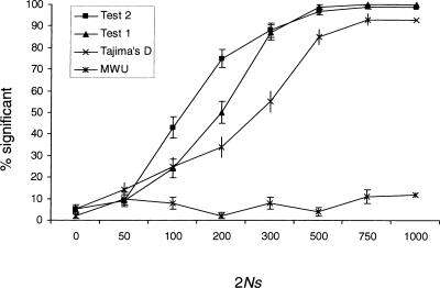
To analyze the statistical properties of the tests proposed here, we conducted extensive simulations. We compare the performance of Tajima's D test and the Mann-Whitney U test (MWU) in a sliding window to the performance of Test 1 and Test 2. We first evaluated the power when the tests are applied to the unfolded frequency spectrum, that is, when an outgroup has been used to infer the ancestral state (Fig. 1). In this case, the MWU test has very little power because a selective sweep increases the frequency of both high-frequency-derived and low-frequency-derived mutations, and reduces the proportion of mutations of intermediate frequency. The power of both Test 1 and Test 2 is higher than the power of Tajima's D, and the power of Test 2 is somewhat higher than the power of Test 1, at least for intermediate values of 2Ns. This is not surprising since Test 2 is based on an explicit model of selective sweeps.

Figure 1.

The proportion of significant results of the four different tests when applied to the unfolded frequency spectrum, as determined by simulations, assuming a region of 250 kb and a single selective sweep. The power is given as a function of the product of the chromosomal population size (2N) and the selection coefficient (s). Error bars indicate ±1 standard deviation. Each point is calculated using 100 replicate simulations.

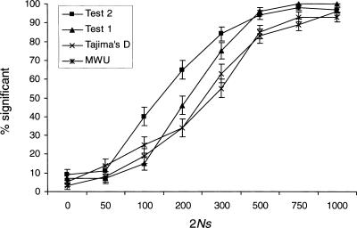
The power to detect a selective sweep based on the folded frequency spectrum is depicted in Figure 2. Tajima's D does not take advantage of outgroup information and is performed identically for unfolded and folded data. The power of the MWU test and Tajima's D test are now comparable, but the power of the other tests is largely unaffected. The reason is presumably that a selective sweep affects both the proportion of high-frequency-derived and low-frequency-derived mutations. It is possible that the increase in information associated with the use of the unfolded frequency spectrum is counteracted by the increase in the number of parameters in models of unfolded frequency spectra. This suggests that the MWU should be performed using the folded, and not the unfolded frequency spectrum, because use of the unfolded frequency spectrum involves additional assumptions regarding the outgroup species and may be sensitive to mis-specifications of ancestral states.

Figure 2.

The proportion of significant results of the four different tests when applied to the folded frequency spectrum (see Fig. 1 for other details).

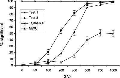
Next we were interested in examining the power and robustness of the test under a demographic model that includes population growth, when the neutral equilibrium model is used as the null model (Fig. 3). In this case, Tajima's D rejects in 100% of the cases, even in the absence of a selective sweep. As shown in Simonsen et al. (1995), and pointed out by Tajima (1989), Tajima's D can detect deviations from the standard neutral model due to both demographic factors and selection. However, Test 1, Test 2, and the MWU test are all much more robust. In fact, all of these tests appear to become conservative under models of population growth. This is fairly remarkable, because population bottlenecks and growth in a population with recombination can produce local troughs in diversity and spikes in linkage disequilibrium that appear almost identical to signatures of selective sweeps (e.g., Barton and Etheridge 2004). Standard methods for detecting selective sweeps, such as Tajima's D, or measures based on levels of LD or population subdivision, suffer from many false positives when a standard neutral model is assumed. However, the tests proposed here have increased robustness because of the use of the global observed frequency spectrum as the background. While the degree of robustness cannot be guaranteed to be as impressive for all other possible models, these results do suggest that tests based on comparing the local frequency spectrum to the global genomic frequency spectrum are attractive in having very high power while having increased robustness to the demographic assumptions.

Figure 3.

The proportion of significant results of the four different tests under population growth, when an equilibrium model is used as the null model. The simulation details are as in Figure 1, but with a 10-fold reduction in population size N generations ago. The null model assumed is a standard neutral equilibrium model without population growth.

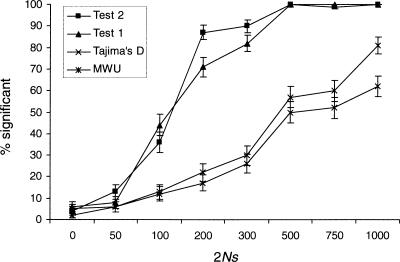
In practical applications, it may be desirable to perform the tests using more realistic demographic models as the null model. If the assumed demographic model is correct, this circumvents the problem of robustness to demographic factors. Although there is considerable uncertainty regarding what the correct model for human demography might be, using more realistic demographic models might nonetheless in many applications be more desirable than the simplistic standard neutral model. Therefore, it might also be of interest to see how the power of the tests compare when the correct demographic model has been used as a null model in the presence of population growth (Fig. 4). Notice that Test 1 and Test 2 in this case have much more power than the MWU test and Tajima's D. Applying Tajima's D test, and possibly other related tests, while correcting for population growth, may lead to tests with very low power.

Figure 4.

The proportion of significant results of the four different tests under population growth, when a growth model is used as the null model. The simulation details are as in Figure 3, but the null model considered is now the correct model, that is, a model with a 10-fold reduction in population size 0.5N generations ago.

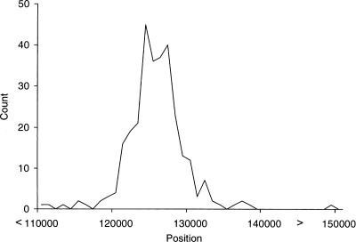
The accuracy of the inference of the locations of the selective sweep is illustrated in Figure 5 based on the significant results under 2Ns = 500, 750, and 1000. Notice that almost all the inferred sweeps are within a window of ∼10 kb centered on the true location of the sweep. While the accuracy of the location of the inferred sweep is strongly dependent on the SNP density and recombination rate, these results suggest that even for genomic SNP data it is possible to identify the location of a selective sweep to a particular gene. For older selective sweeps, the accuracy may be lower.

Figure 5.

The distribution of the inferred location of the selective sweep in significant simulations with 2Ns = 500, 750, and 1000. The true location of the selective sweep is at position 125,000.

Robustness of Test 2

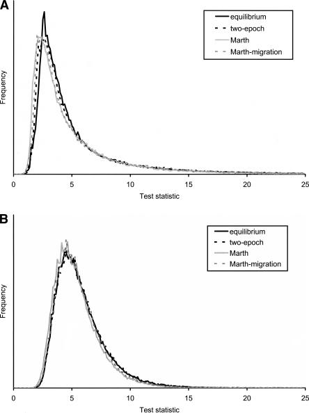
To evaluate the robustness of Test 2 further, we determined the distribution of the test statistic for various realistic models of human demography, such as the model of divergence and population growth explored by Marth et al. (2004). To save computational time, we simulated only 200 SNPs in each replicate. Results for high (ρ =2NR =10^–3) and low (ρ =2NR = 0) values of the recombination rate are shown in Figure 6. Notice that the null distributions are very similar for all investigated demographic models. This suggests that Test 2 has a very high degree of robustness against demographic assumptions. Close inspection of the tails reveals some differences that will affect the critical values of tests performed at the 5% and 1% significance levels. However, it is important to notice that for both high recombination rates and low recombination rates, the standard neutral model provides the most conservative critical values. This means that using the standard neutral null model, when the Marth et al. (2004) model is correct, will lead to a conservative test. In most cases, this will be a desirable property, and we recommend use of the standard neutral equilibrium model when applying this test to human data.

Figure 6.

The null distribution of Test 2 different tests under different demographic models described in the text and a recombination rate of (A) 2NR = 0 and (B) 2NR =10^–3 per base pair.

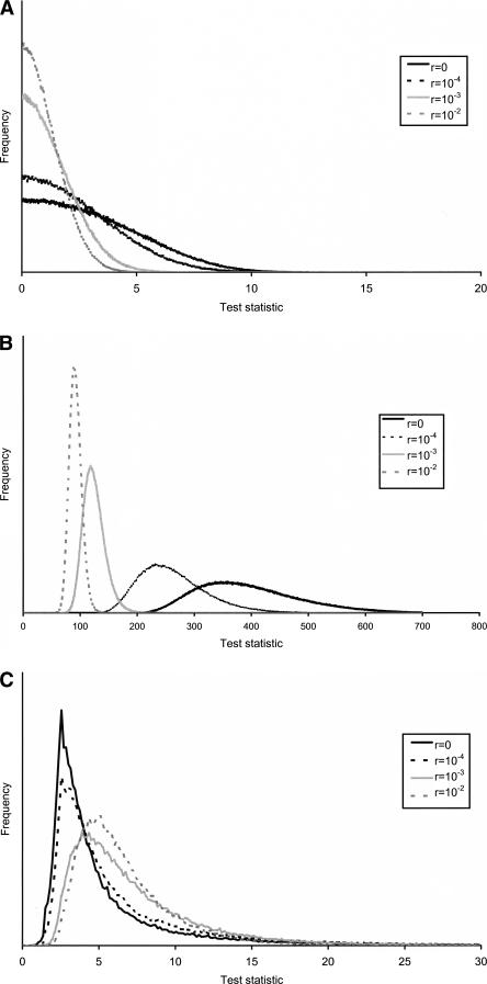
We also examined the null distribution under varying assumptions regarding the recombination rate, to investigate the robustness of Test 1, Test 2, and the MWU test to such assumptions (Fig. 7). The distribution of the test statistic of the MWU test (Fig. 7A) shows weak dependence on the recombination rate when the rate of recombination is high, but strong dependence when the recombination rate is low. Clearly, accurate estimates of the recombination rate are important when applying this test. Test 1 shows even stronger dependence on the recombination rate (Fig. 7B). If the recombination rate assumed is higher than the true recombination rate, application of this test will lead to an elevated type I error. In contrast to Test 1, Test 2 has a very high degree of robustness to assumptions regarding the recombination rate (Fig. 7C). As in the case of the other tests, R =0 provides the most conservative assumption. The extreme difference between the behavior of Test 1 and Test 2 tests can probably best be explained by noting that much of the information for Test 2 comes from the spatial pattern along the sequence, and that distances for this test depend on the selection coefficient, which is a free parameter. Wrong assumptions about the recombination rate will then lead to biased estimates of the selection coefficient, but will not have a strong effect on the null distribution of the test statistic (Kim and Nielsen 2004).

Figure 7.

The null distribution of (A) the Mann-Whitney U (MWU) test, (B) Test 1, and (C) Test 2 under varying assumptions regarding the recombination rate.

Analysis of Seattle SNP data

To illustrate the method, we first apply it to 148 gene regions for 24 African American individuals and 23 Europeans from the Seattle database (see Methods for details).

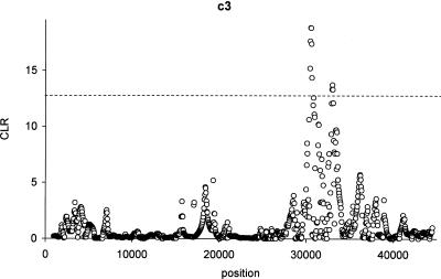
Results for the gene regions with p-values < 0.05 are shown in Table 1. Figure 8 also shows the maximized composite likelihood function along the length of the gene region of the gene showing the strongest evidence for a selective sweep, C3. The maximum composite likelihood estimate of the location of the sweep falls approximately in an intron at position 30,525. This intron contains several insertion/deletion differences when compared to the chimpanzee sequence and is a region associated with alternative splicing.

Table 1.

The genes among 148 genes from the Seattle database showing the strongest evidence for a selective sweep based on Test 2

Locus	Composite LR	p-value
C3	18.80	0.01
VCAM1	12.67	0.03
PPARA	9.50	0.03
TNFAIP1	8.35	0.04

Figure 8.

The maximized composite likelihood surface calculated for the c3 gene calculated from the Seattle SNP database (SeattleSNPs, http://pga.gs.washington.edu [Feb. 2004]). The dotted line indicates the 5% cutoff value as determined by simulations under a standard neutral equilibrium model.

These data have previously been examined by other researchers for the purpose of detecting selective sweeps. Akey et al. (2002) used Tajima's D and related statistics to test for deviations from a neutral model. They detected several genes with extreme values of the test statistic, although not C3. One of the main causes for the discrepancy is presumably that the current analysis was applied to the pooled data from all populations while the analysis in Akey et al. (2002) was applied to data from each population individually.

Analysis of HapMap data

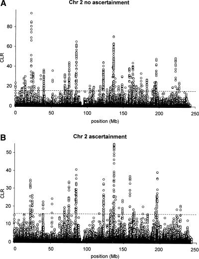
To further illustrate the utility, we analyzed data from the Hap-Map project (The International HapMap Consortium 2003) for Chromosome 2. We show results for Test 2, with and without a correction for ascertainment bias (Fig. 9A,B).

Figure 9.

The maximized composite likelihood surface calculated for data from Chromosome 2 from the HapMap project (The International HapMap Consortium 2003). The dotted line indicates the 5% cutoff value as determined by simulations under a standard neutral equilibrium model. Results are shown with (B) and without (A) a correction for ascertainment bias.

The main effect of the ascertainment bias correction of the HapMap data is to reduce the composite likelihood ratio value for several of the significant peaks (Fig. 9). It also changes the relative height of the peaks, of the likelihood function, depending on the underlying ascertainment sample size in the region. This illustrates the importance of correcting for ascertainment biases, and suggests that lack of correction for ascertainment bias may lead to excess false positives.

The genes identified to lie within a confidence region for a selective sweep are listed in Table 2. The major peak (at position 1.36 × 10⁸) of the composite likelihood surface is centered on the lactase (LCT) locus. The evidence for selection on the lactase locus dates back to the early seventies (e.g., Cavalli-Sforza 1973), and recently SNP data have provided strong evidence for selection on lactase (Bersaglieri et al. 2004). Presumably, as domestication of dairy animals allowed for increased consumption of milk, mutations that retain an ability to digest lactose in adults were selectively favored and rose to high frequency recently and quickly.

Table 2.

Sweep and genes located inside a 95% confidence interval for the location of a selectivve sweep in Chromosome 2 or the HapMap data

Location	CLR	Genes
13.6 × 107	55.0	ZRANB3, R3HDM, UBXD2, LCT, MCM6, DARS, CXCR4
8.47 × 107	40.7	SUCLG1
19.6 × 107	39.3
15.8 × 107	37.0	ACVR1C
12.2 × 107	35.2	MKI67I, TSN
2.18 × 107	34.7
7.47 × 107	33.7	RTKN, HMGA1L4, WBP1, GCS1, MRPL53, LBX, PCGF1, TLX2, DQX1, AUP1, PRSS25, LOXL3, DOK1, SEMA4F
2.45 × 107	26.1	ITSN2
13.9 × 107	25.5
5.17 × 107	24.3
14.8 × 107	23.6	ACVR2A
3.94 × 107	22.5	CDKL4, MAP4K3
13.5 × 107	21.7
22.8 × 107	20.6	COL4A3
17.6 × 107	20.0
6.88 × 107	19.3	GPR73
14.4 × 107	19.2	KYNU
19.3 × 107	19.0
22.3 × 107	18.5
16.3 × 107	18.4	KCNH7
13.2 × 107	18.1	H2-ALPHA, FKSG30
16.4 × 107	17.0	FIGN
11.6 × 107	16.1	DPP10

There are several disease factors on the gene list in Table 2, including COL4A3, a known disease factor for Alport syndrome. The peak at location 14.4 × 10⁷ is associated with the KYNU gene encoding kynurenine hydrolase. Elevated levels of this enzyme are associated with cerebral and systemic inflammatory conditions. A peak at position 12.2 × 10⁷ is located on the TSN gene. The protein encoded by this gene, translin, binds to single-stranded DNA ends generated by staggered breaks, such as those occurring at recombination and translocation breakpoints. A peak at location 1.71 × 10⁷ is located on the DPP10 gene, a gene that is primarily expressed in the brain but also has been implicated as a disease factor for asthma. There are several other genes that are specific to the brain or overexpressed in neuronal tissue. A peak at location 7.5 × 10⁷ is located on the SEMA4F gene, a gene that functions in axon guidance. ACVR1C, the only gene in the confidence region under the peak with the fourth highest CLR, is a type I receptor for TGFβ that plays an unknown role during mammalian brain development.

Discussion

The modification of the Kim and Stephan (2002) method presented here (Test 2) provides an attractive test for detecting selective sweeps. It has unprecedented robustness to demographic factors and assumptions regarding the recombination rate. At the same time, it has considerable power to detect a recent selective sweep, it is computationally fast enough to be applied to large-scale genomic data, and it can incorporate ascertainment biases. Nonetheless, as with all other neutrality tests, it is always important to consider potential causes of spurious significant results. Test 2 was here shown to be remarkably robust to demographic assumptions involving a change in population size and some realistic models of human demography (e.g., the Marth et al. 2004 model). However, this does not eliminate the possibility that there are other demographic models, not investigated here, under which the test is not robust. Any real application of the test should carefully consider the underlying demographics for the populations/species of interest when establishing null models and interpreting the results. Nonetheless, using a standard neutral equilibrium model seems to be a fairly safe approach in the analysis of human data using Test 2.

Beyond demographic factors, significant results of the neutrality tests considered here may be caused by other types of selection than a selective sweep. Test 2 may in this sense give spurious results if other types of selection are acting locally to mimic the signature of a selective sweep. It is unknown to what degree selection against slightly deleterious mutations could mimic the spatial pattern providing the power of Test 2.

Test 2 is designed specifically to detect a recent selective sweep and may have very little power to detect other types of selection, such as balancing selection. It may, therefore, be preferable to use other methods, such as Test 1 or the MWU-based test, if other types of selection are of interest. Alternatively, extensions of Test 2 that specifically accommodate different modes of selection, such as balancing selection, could be implemented.

Ascertainment was here modeled explicitly for the HapMap data based on information regarding the empirical distribution of ascertainment sample sizes. However, many complexities of the ascertainment procedure for the HapMap data were ignored. Nonetheless, it is clear from the current results that ascertainment, and its correction, seems to matter, even for Test 2. Also, it is clear that selective sweep mapping using Test 2 has great potential for identifying regions in the human genome that have been targeted by recent sweeps. The simplified analysis performed here found the strongest evidence for selection associated with the lactase locus, which previously has been demonstrated to be under selection, but it also identified several other interesting potential targets of selective sweeps. We hope that further analysis of extensive genome-wide human polymorphism data, especially when combined with full information regarding the ascertainment scheme, may help determine which genes in the human genome have been targeted by selective sweeps.

Methods

Simulations

The sliding window sizes for the MWU test, Tajima's D test, and Test 1 were chosen based on preliminary runs to maximize the power of the tests. No choice of window size is necessary for Test 2. We first simulated data using the method of Kim and Stephan (2002) for a sample of 50 chromosomes. These simulations allowed us to model a recent selective sweep for varying values of 2Ns. The recombination rate was assumed to be 0.01 per nucleotide, and 250,000 base pairs were simulated under a value of θ = 0.005. The selective sweep, of strength α, was placed in the center of the chromosome. Critical values were found by repeatedly simulating data from a standard neutral coalescence model under values of θ estimated from the data using the number of segregating sites and the true values of the recombination rate. Simulations were performed using the standard coalescent simulation algorithm (e.g., Hudson 2002).

To determine the power in the presence of population growth, we modified the simulation method of Kim and Stephan (2002) to incorporate changes in the population size. We considered a model with a change in population size 0.5 coalescence units in the past, such that the population size fell to 10% of the current size. Again, critical values were obtained using a standard neutral model with estimated values of θ.

We investigated the robustness of Test 2 further, using an additional set of simulations. In all, 100,000 new data sets of 200 SNPs were simulated for varying assumptions regarding demography and recombination. For each 200-SNP window, we performed Test 2 using the remaining data sets to provide the background frequency spectrum. We examined four demographic conditions:

1. The standard neutral equilibrium model.

2. A two-epoch growth model using the estimates in Williamson et al. (2005) with an decrease in population size to 16% of the current population size 0.0088N generations ago.

3. A model of divergence and population growth between two populations with population size parameters estimated from human SNP data by Marth et al. (2004). This model assumes that the Chinese, European, and African populations have diverged from the ancestral population ∼0.05N generations ago and that the divergence event was associated with a bottleneck (see Marth et al. 2004 for more details).

4. The Marth et al. (2004) model with migration between populations at a rate of five individuals per generation.

Ascertainment was also modeled in these simulations using varying discovery sample sizes corresponding to the ascertainment method used for the Perlegen data (Hinds et al. 2005). The simulations exploring robustness to the recombination rate were performed similarly.

Construction of confidence regions

Confidence regions for the location of a selective sweep in the HapMap data were constructed based on the composite likelihood ratio score (t). Using the pooled simulation results for the whole chromosome simulations under 2Ns = 500, 750, and 1000, a cutoff (t_0.05) for each selective sweep was found such that all positions with t > t_0.05 were included in the region and the probability that the region contained the true position was 0.95. Because the likelihood surface usually has multiple peaks close to each other, and because the likelihood was calculated on a grid along the sequence, in practice, the confidence regions were formed by taking the union of line segments of lengths around points with t > t_0.05, where is the maximum likelihood estimate for the midpoint of the interval. This procedure is not intended to identify the number of selective sweeps. Such a procedure would require the modeling of multiple simultaneous sweeps. Our approach for constructing confidence regions may also be sensitive to assumptions regarding SNP density and other factors. However, this procedure does define a computationally tractable method that forms accurate confidence regions in the simulated data, and is suitable for determining the most likely set of genes that have been targeted by selective sweeps.

Analysis of Seattle SNP data

Data were obtained from the Seattle database (SeattleSNPs, http://pga.gs.washington.edu [Feb. 2004]) for 24 African American individuals and 23 Europeans. We applied Test 2 to each gene with the objective of identifying selective sweeps, and the possible location of a selective sweep within each data set. For each gene, the composite likelihood function was calculated on a grid of 10,000 positions along the length of the gene. For each position, the parameter α was then optimized numerically. The test statistic used to test for selective sweeps in a gene was the maximum composite likelihood value optimized over all possible positions and all possible values of α, compared to the composite likelihood of the neutral null model. Critical values were obtained by simulating 100 neutral new data sets with (scaled) recombination rates and values of θ estimated from the data, assuming homogenous recombination rates among regions. For each simulated data set, the entire inference procedure was repeated to generate new maximum composite likelihood values. p-values were then estimated by comparing the maximum composite likelihood value from the real data set, to the distribution observed in the simulated data sets. θ was estimated using the number of segregating sites (Watterson 1975), and the (scaled) recombination rate was estimated using the median of the posterior expectation based on the method implemented in PHASE (Stephens et al. 2001), giving an estimate of ρ = 7.366 × 10^–4 per base pair. Given the apparent robustness of Test 2 to demographic assumptions, and the fact that the standard neutral model provides a more conservative assumption than any of the more realistic models investigated (e.g., Marth et al. 2004), no attempt to correct for demographic factors was performed. This simulation procedure automatically corrects for multiple tests within each gene.

Analysis of HapMap data

There are several challenges involved in the analysis of the Hap-Map data. The data set is large but has been obtained using an ascertainment procedure that may bias the results. The main effect we take into account is the SNP ascertainment sample size of each SNP. This is done using equations 7 and 8 based on ascertainment sample size information provided by J.C. Mullikin, National Institutes of Health. However, as this analysis is only provided for the purpose of illustrating the method, we do not attempt a more detail modeling of the ascertainment scheme. The real ascertainment is more complicated than modeled here involving a so-called double-hit approach and a comparison with a chimpanzee sequence. Here, we simply use the empirical distribution of ascertainment depths (d in equation 8) for each SNP. Given this information, the ascertainment correction is done by directly applying equations 7 and 8 to the data as a modified composite likelihood function. The resulting likelihood surface is, as previously, optimized with respect to α to provide a profile composite likelihood function along the length of the chromosome. The values of d for individual SNPs are available from the authors on request. The mean and standard deviation of the number of chromosomes (d) in the alignment in the analyzed ascertainment data is 5.94 and 2.22. There was some regional variation in the value of d along the chromosome. The mean value of d calculated in windows of 100 SNPs varied from 4.6 to 7.1.

To obtain critical values, we again use neutral coalescence simulations, with parameter values estimated from the real data. The critical value obtained for the HapMap data is the maximum composite likelihood ratio observed in the entire chromosome. This procedure then automatically controls for multiple tests.

We explicitly model the ascertainment process when simulating the data (e.g., Nielsen et al. 2004). Also, because it is not computationally feasible to simulate an entire chromosome using coalescent simulations, we divided the chromosome into 1-Mb segments and simulated data independently for each segment. To distinguish between different sweeps, we heuristically assumed that two peaks at a distance of more than from each other represent different sweeps. The previously discussed confidence region method was used to assign genes to each putative sweep.

References

- Akashi, H. 1999. Inferring the fitness effects of DNA mutations from patterns of polymorphism and divergence: Statistical power to detect directional selection under stationarity and free recombination. Genetics 151: 221–238. [DOI] [PMC free article] [PubMed] [Google Scholar]
- Akey, J.M., Zhang, G., Zhang, K., Jin, L., and Shriver, M.D. 2002. Interrogating a high-density SNP map for signatures of natural selection. Genome Res. 12: 1805–1814. [DOI] [PMC free article] [PubMed] [Google Scholar]
- Barton, N.H. 1998. The effect of hitch-hiking on neutral genealogies. Genet. Res. 72: 123–133. [Google Scholar]
- Barton, N.H. and Etheridge, A.M. 2004. The effect of selection on genealogies. Genetics 166: 1115–1131. [DOI] [PMC free article] [PubMed] [Google Scholar]
- Bersaglieri, T., Sabeti, P.C., Patterson, N., Vanderploeg, T., Schaffner, S.F., Drake, J.A., Rhodes, M., Reich, D.E., and Hirschhorn, J.N. 2004. Genetic signatures of strong recent positive selection at the lactase gene. Am. J. Hum. Genet. 74: 1111–1120. [DOI] [PMC free article] [PubMed] [Google Scholar]
- Cavalli-Sforza, L. 1973. Analytic review: Some current problems of population genetics. Am. J. Hum. Genet. 25: 82–104, 156. [PMC free article] [PubMed] [Google Scholar]
- Clark, A.G., Glanowski, S., Nielsen, R., Thomas, P.D., Kejariwal, A., Todd, M.A., Tanenbaum, D.M., Civello, D., Lu, F., Murphy, B., et al. 2003. Inferring non-neutral evolution from human–chimp–mouse orthologous gene trios. Science 302: 1960–1963. [DOI] [PubMed] [Google Scholar]
- Durrett, R. and Schweinsberg, J. 2004. Approximating selective sweeps. Theor. Popul. Biol. 66: 129–138. [DOI] [PubMed] [Google Scholar]
- Fay, J.C. and Wu, C.-I. 2000. Hitchhiking under positive Darwinian selection. Genetics 155: 1405–1413. [DOI] [PMC free article] [PubMed] [Google Scholar]
- Gilad, Y., Rosenberg, S., Przeworski, M., Lancet, D., and Skorecki, K. 2002. Evidence for positive selection and population structure at the human MAO-A gene. Proc. Natl. Acad. Sci. 99: 862–867. [DOI] [PMC free article] [PubMed] [Google Scholar]
- Harr, B., Kauer, M., and Schlötterer, C. 2002. Hitchhiking mapping: A population-based fine-mapping strategy for adaptive mutations in Drosophila melanogaster. Proc. Natl. Acad. Sci. 99: 12949–12954. [DOI] [PMC free article] [PubMed] [Google Scholar]
- Hinds, D.A., Stuve, L.L., Nilsen, G.B., Halperin, E., Eskin, E., Ballinger, D.G., Frazer, K.A., and Cox, D.R. 2005. Whole-genome patterns of common DNA variation in three human populations. Science 307: 1072–1079. [DOI] [PubMed] [Google Scholar]
- Hudson, R.R. 2002. Generating samples under a Wright-Fisher neutral model. Bioinformatics 18: 337–338. [DOI] [PubMed] [Google Scholar]
- The International HapMap Consortium. 2003. The International HapMap Project. Nature 426: 789–796. [DOI] [PubMed] [Google Scholar]
- Jensen, J.D., Kim, Y., Dumont, V.B., Aquadro, C.F., and Bustamante, C.D. 2005. Distinguishing between selective sweeps and demography using DNA polymorphism data. Genetics 170: 1401–1410. [DOI] [PMC free article] [PubMed] [Google Scholar]
- Kaplan, N.L., Hudson, R.R., and Langley, C.H. 1989. The `hitchhiking effect' revisited. Genetics 123: 887–899. [DOI] [PMC free article] [PubMed] [Google Scholar]
- Kim, Y. and Stephan, W. 2002. Detecting a local signature of genetic hitchhiking along a recombining chromosome. Genetics 160: 765–777. [DOI] [PMC free article] [PubMed] [Google Scholar]
- Kim, Y. and Nielsen, R. 2004. Linkage disequilibrium as a signature of selective sweeps. Genetics 167: 1513–1524. [DOI] [PMC free article] [PubMed] [Google Scholar]
- Lewontin, R.C. and Krakauer, J. 1973. Distribution of gene frequency as a test of the theory of the selective neutrality of polymorphisms. Genetics 74: 175–195. [DOI] [PMC free article] [PubMed] [Google Scholar]
- Marth, G.T., Czabarka, E., Murvai, J., and Sherry, S.T. 2004. The allele frequency spectrum in genome-wide human variation data reveals signals of differential demographic history in three large world populations. Genetics 166: 351–372. [DOI] [PMC free article] [PubMed] [Google Scholar]
- Maynard Smith, J. and Haigh, J. 1974. The hitch-hiking effect of a favourable gene. Genet. Res. 23: 23–35. [PubMed] [Google Scholar]
- Nielsen, R. 2004. Population genetic analysis of ascertained SNP data. Hum. Genomics 1: 218–224. [DOI] [PMC free article] [PubMed] [Google Scholar]
- Nielsen, R. and Signorovitch, J. 2003. Correcting for ascertainment biases when analyzing SNP data: Applications to the estimation of linkage disequilibrium. Theor. Pop. Biol. 63: 245–255. [DOI] [PubMed] [Google Scholar]
- Nielsen, R., Todd, M.J., and Clark, A.G. 2004. Reconstituting the frequency spectrum of ascertained SNP data. Genetics 168: 2373–2382. [DOI] [PMC free article] [PubMed] [Google Scholar]
- Parsch, J., Meiklejohn, C.D., and Hartl, D.L. 2001. Patterns of DNA sequence variation suggest the recent action of positive selection in the janus–ocnus region of Drosophila simulans. Genetics 159: 647–657. [DOI] [PMC free article] [PubMed] [Google Scholar]
- Przeworski, M. 2002. The signature of positive selection at randomly chosen loci. Genetics 160: 1179–1189. [DOI] [PMC free article] [PubMed] [Google Scholar]
- Przeworski, M. 2003. Estimating the time since the fixation of a beneficial allele. Genetics 164: 1667–1676. [DOI] [PMC free article] [PubMed] [Google Scholar]
- Sabeti, P.C., Reich, D.E., Higgins, J.M., Levine, H.Z., Richter, D.J., Schaffner, S.F., Gabriel, S.B., Platko, J.V., Patterson, N.J., McDonald, G.J., et al. 2002. Detecting recent positive selection in the human genome from haplotype structure. Nature 419: 832–837. [DOI] [PubMed] [Google Scholar]
- Simonsen, K.L., Churchill, G.A., and Aquadro, C.F. 1995. Properties of statistical tests of neutrality for DNA polymorphism data. Genetics 141: 413–429. [DOI] [PMC free article] [PubMed] [Google Scholar]
- Stephan, W., Wiehe, T.H.E., and Lenz, M.W. 1992. The effect of strongly selected substitutions on neutral polymorphism: Analytical results based on diffusion theory. Theor. Pop. Biol. 41: 237–254. [Google Scholar]
- Stephens, M., Smith, N., and Donnelly, P. 2001. A new statistical method for haplotype reconstruction from population data. Am. J. Hum. Genet. 68: 978–989. [DOI] [PMC free article] [PubMed] [Google Scholar]
- Tajima, F. 1989. The effect of change in population size on DNA polymorphism. Genetics 123: 597–601. [DOI] [PMC free article] [PubMed] [Google Scholar]
- Watterson, G.A. 1975. On the number of segregating sites in genetical models without recombination. Theor. Pop. Biol. 7: 256–276. [DOI] [PubMed] [Google Scholar]
- Williamson, S.H., Hernandez, R., Fledel-Alon, A., Zhu, L., Nielsen, R., and Bustamante, C.D. 2005. Simultaneous inference of selection and population growth from patterns of variation in the human genome. Proc. Natl. Acad. Sci. 102: 7882–7887. [DOI] [PMC free article] [PubMed] [Google Scholar]
- Wootton, J.C., Feng, X., Ferdig, M.T., Cooper, R.A., Mu, J., Baruch, D.I., Magill, A.J., and Su, X.-Z. 2002. Genetic diversity and chloroquine selective sweeps in Plasmodium falciparum. Nature 418: 320–323. [DOI] [PubMed] [Google Scholar]
Web site references
- http://pga.gs.washington.edu; the Seattle SNP database [Feb. 2004]—SeattleSNPs. NHLBI Program for Genomic Applications, SeattleSNPs, Seattle, WA.