Wildfires, complexity, and highly optimized tolerance

Abstract

Recent, large fires in the western United States have rekindled debates about fire management and the role of natural fire regimes in the resilience of terrestrial ecosystems. This real-world experience parallels debates involving abstract models of forest fires, a central metaphor in complex systems theory. Both real and modeled fire-prone landscapes exhibit roughly power law statistics in fire size versus frequency. Here, we examine historical fire catalogs and a detailed fire simulation model; both are in agreement with a highly optimized tolerance model. Highly optimized tolerance suggests robustness tradeoffs underlie resilience in different fire-prone ecosystems. Understanding these mechanisms may provide new insights into the structure of ecological systems and be key in evaluating fire management strategies and sensitivities to climate change.

From the scale of individual plants up to the entire planet, fire plays a central role in structuring natural terrestrial systems. Although the importance of fire is generally under appreciated (1), consistent fire-related patterns can be observed everywhere. Exposure to fire over evolutionary time scales has led to similar adaptations in widely separated species (2), including strategies of fire resistance (e.g., thick protective bark) and even fire dependence for regeneration. For example, many plant species in fire-prone environments require smoke-related chemical cues for seed germination (3–5), and serotiny (i.e., seed dormancy until cones are exposed to heat) is common to several conifers (6, 7). Effects of fire can also be observed at the global scale, influencing the distribution of different vegetation types and entire biomes (8, 9). Although we have a moderate understanding of what controls fire behavior and its effects at different scales (Fig. 1), much less is known about interactions between these scales and how emergent properties of ecosystems are generated. Despite several decades of work on ecosystem patch dynamics generated by fire or other disturbances (10–13), the importance of spatial patterns and processes at different scales remains at the forefront of modern ecology (14–16).

Fig. 1.

Controls on fire at different scales. Dominant factors that influence fire at the scale of a flame, a single wildfire, and a fire regime. This is an extension of the traditional “fire triangle” concept (20, 21), here including broad scales of space and time, the feedbacks that fire has on the controls themselves (small loops), as well as feedbacks between processes at different scales (arrows).

At relatively broad spatiotemporal scales, many fire size distributions exhibit roughly power law statistics, in which the probability P(l) of a fire greater than or equal to size l is given by the inverse size raised to a power α: P(l) ∼ l^–α. The surprising consistency of this form provides a starting point for links to models and mechanisms for structure in complex natural systems exposed to recurring wildfires (17–19). The fire regime of an ecosystem is the collective outcome of multiple drivers, such as ignition patterns, climate, and vegetation characteristics (Fig. 1). The influence of fire then feeds back to affect vegetation distributions. The small loops in Fig. 1 illustrate the strong feedbacks between fire and the control parameters, and the arrows emphasize the feedbacks that act between scales. Together these factors govern the evolution of a fire regime, leading to characteristic patterns and approximate recurrence intervals for fires of different sizes, reflecting aspects of ecosystem structure at a relatively coarse resolution. Although a fire regime is also characterized by distributions of fire frequencies, intensities, and timing, many of these factors covary, and emphasis at the ecosystem scale is often on fire sizes.

Highly optimized tolerance (HOT) is a conceptual framework for examining organization and structure in complex systems (18). Theoretically, HOT builds on models and mathematics from physics and engineering, and identifies robustness tradeoffs as a principle underlying mechanism for complexity and power law statistics. HOT has been discussed in the context of a variety of technological and natural systems, including wildfires (18, 22). A quantitative prediction for the distribution of fire sizes has come from an extremely simple analytical HOT model, referred to as the PLR (probability–loss–resource) model (22). As a precursor to results presented later in this article, Fig. 2 demonstrates the PLR prediction and truncated power law statistics (23) for several fire history catalogs. This plot represents the raw data as rank or cumulative frequency of fires P(l) greater than or equal to a given size as a function of size l measured in km². In the forestry and ecology literature, fire size statistics have been analyzed primarily for correlations between fire size and other variables, such as climate, vegetation type, or suppression by humans (see, e.g., ref. 24–26). The fact that fire statistics are indeed described by power laws was identified relatively recently (27), initially in the context of self-organized criticality (17). A more accurate statistical fit was later proposed by using HOT (22). A very recent analysis of fire size distributions has confirmed power law fits for many parts of the United States (28), but the mechanism generating these consistent patterns is still under investigation.

Fig. 2.

Cumulative fires P(l) vs. size l and comparison with the PLR HOT model. The four data sets (points) represent our reanalysis of unscaled data obtained from ref. 27 and include 4,284 fires on U.S. Fish and Wildlife Service lands (1986–1995; black circles), 120 of the largest fires in the western United States (1150–1960) determined from tree ring data (blue circles), 164 fires in Alaskan boreal forests (1990–1991; red squares), and 298 fires in the Australian Capital Territory (1926–1991; green circles). The data represents rank order frequency and are well described by the PLR model (Eq. 2) with d = 2 (solid black curves passing through points). The straight dashed line with slope –0.15 is shown for comparison and corresponds to the exponent of the self-organized criticality forest fire model (27). The dashed line of slope –0.5 corresponds to the asymptotic exponent for the PLR HOT model (22).

There are several striking features of Fig. 2 that will be discussed in more detail and which motivate the rest of this article. One highlight is the nearly identical form (i.e., the same exponent α for the power law) of many fire history data sets, suggesting some common mechanism, despite the diversity of the data from very different fire-prone environments. Another notable aspect is the equally perfect fit of the HOT PLR model to the data. The PLR model is both extremely simple and explicitly based on constrained optimization, so the striking fit raises a variety of questions that we can only begin to address. What is the significance of the consistent fire size statistics for different ecosystems? Even if an ecosystem appears to be optimized in some sense, how can this be captured in a model as simple as PLR? Is the fit accidental, or has PLR captured an essential tradeoff in the structure of fire-prone ecosystems?

Each of these questions is by itself an enormous and complicated research problem, and we primarily aim to frame the questions and offer small steps in promising directions. Specifically, our approach is to reexamine and extend the PLR model statistical fits to several fire history catalogs. To investigate parameters that are influential in generating different fire size distributions, we focus on a long-term simulation model (HFire) (29), which represents an intermediate level of resolution in the processes controlling fire occurrence and propagation in an ecosystem. This model has no explicit “optimization” but instead simply aims to capture, as faithfully as available data and standard models allow, the various elements known to affect the behavior of individual fires. Our working hypothesis is that the natural feedbacks associated with ecological processes over time have led to vegetation patterns that are well suited (if not completely “optimized”) to the local fire regime, so that by modeling current conditions with reasonable fidelity, we may be capturing the net result of some underlying mechanism for ecosystem resilience. We end by focusing on inherent tradeoffs that influence the spread of wildfires and ecological responses to them, comparing in one direction with the simple PLR model, and in the other direction with the much greater complexity of real ecosystems. Although the remaining gaps in knowledge are still large, the simulated and historical data analyzed here allow insights to the above questions, indicating promising areas for further research.

PLR Model and Wildfire Statistics

HOT emphasizes specialized configurations of interacting components, tuned via biological mechanisms (30–32) or engineering design (33, 36, 74, 75) to be robust to fluctuations and variability in the environment (37, 38). A key concept from HOT theory is that tuning for robustness involves tradeoffs subject to constraints and that the very mechanisms and interdependencies which increase robustness to common events also introduce new sensitivities or fragilities to rare or unanticipated disturbances. In ecological applications the word “optimization” is perhaps more aptly replaced by “organization,” reflecting the distinction between HOT and random, disorganized configurations, and highlighting the importance of structured interdependencies that evolve via feedback among and between biotic and abiotic variables. It should be noted here that evidence of organization does not imply a designer; indeed, optimization per se is not essential for HOT to apply. The most salient outcome of HOT models are the consequences associated with more resources being allocated to common events and less to rare ones. In terrestrial ecosystems, this tendency may lead to dominant patterns of species distributions and plant community structures that reflect the prevailing environmental conditions, whereas other patterns may reflect acclimation to marginal conditions or adaptations to infrequent extreme events. Such partitioning and tradeoffs are likely to arise in any sensible model involving design or evolution of resilient systems.

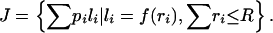
The PLR model is the simplest, most abstract HOT model, and complete mathematical details are presented elsewhere (22, 39). Here, we briefly summarize the basic setup and solution, which we use in this article to compare wildfire data with the HFire simulations. In the context of a managed forest, “losses” represent areas burned, whereas “resources” would reflect effort spent to minimize those losses on average. The PLR model has event categories i with relative probability p_i and loss l_i, which is a function l_i = f(r_i) solely of the resources r_i that are allocated to the category. For wildfires, the resources vs. loss relationship is assumed to be , which incorporates a cutoff at small fire sizes, and normalizes so that 0 ≤ r_i ≤ 1 with f (1) = 0, and c a constant. The dimensionality here is that of the burnable substrate, d = 2, which arises from the characterization of fire shapes as roughly two-dimensional, compact, area-filling regions, enclosed by one-dimensional perimeters at which fire is extinguished. The resources that may constrain fire sizes are assumed to scale with the linear length of the perimeter, leading to this form of f(r_i) (22, 39), and are subject to an overall constraint r_i ≤ R on the total resources R that are available. The PLR solution then divides the resources in a manner that minimizes the expected burn loss J over the spectrum of possible events:

[1]

This HOT PLR model can be solved analytically (22) and in the limit of large numbers of events has a continuous approximation (18, 39) as a cumulative distribution P(l) = Prob(size > l) of the form

[2]

with α = 1/d = 1/2. This form, which is approximately a power law P(l) ∼ l ^–α, holds over a range of magnitudes between small (C) and large (L) size cutoffs (23), representing physical or observational limits on different ends of the fire size spectrum, the only “free” parameters in the model. The constant A normalizes the units of P, which is typically either the rank or cumulative probability, and thus depends on the number of events in a data record. The curves in Fig. 2 represent just such cumulative probability vs. loss statistics for fires with l_i the area burned in a fire, and the data are compared with the formula in Eq. 2.

As has been recognized before (18), the fit between PLR predictions and a variety of real data in Fig. 2 is remarkable, given the severe abstractions involved. In the PLR model, events are not assumed to have any intrinsic differences other than their probability of occurrence, and thus different losses are entirely due to the distribution of resources. More realistic models (e.g., HFire) would include additional variation in all of the aspects of event initiation and propagation, as suggested by Fig. 1. Our aim here is to use the consistency between PLR predictions and real data to motivate a deeper examination of more mechanistic modeling and additional details of real wildfires.

Additional wildfire data we analyzed come from the mapped fire history of Los Padres National Forest (LPNF) (25, 40), and it provides a baseline for the HFire simulations described in the next section. LPNF is a relatively large region (8,700 km²) in central coastal California, and it is dominated by chaparral shrublands, a plant community with many fire-adapted species. To compare the LPNF data with the HOT PLR prediction (Eq. 2), the cutoff values chosen are C = 0.1 and L = 1,000, which are roughly the smallest (0.1 km²) and largest (890 km²) fire sizes in the database, respectively. The LPNF data record (Fig. 3) has ≈800 fires, with a total 9,900 km² burned over an 85-yr period of record. The median fire size in this data set is 0.8 km², the mean is 12 km², and the SD is 55 km². These large ratios between median, mean, and SD reflect the high variability of the data, which is captured by the coefficient of variation CV = SD/mean = 55/12 = 4.6. [For an exponential distribution, median/mean = ln(2), and CV = 1.] Of the total 9.900 km² of fires, half of the burned area occurs in the largest 15 events, comprising <2% of the fires. The largest 124 fires, which constitute 15% of the total number of fires, are responsible for 90% of the burned area. Thus, the fire regime is dominated by the rare, large events (25), similar to the other data sets (27) in Fig. 2.

Fig. 3.

Fire size statistics for LPNF, HFire, and PLR and data collapse for all data sets. Cumulative number of fires versus fire size for the LPNF (1911–1995; blue dots) and the 500-yr HFire simulation (red dots) in the Santa Monica Mountains. Data and simulations agree well, aside from the few largest fires (see text). Both LPNF and HFire data are well described by the PLR HOT model with d = 2 and appropriate large scale cutoffs. Only the LPNF PLR fit is shown (solid black curve). The family of curves above the unscaled data illustrates the collapse when the four data sets from Fig. 2 are combined with the three data sets here and shifted horizontally for size, and vertically for rate, to overlap.

The approximate power laws shown here are important for several reasons. Most fires in the data sets are relatively small, and many others are so small that they are not even recorded in wildfire catalogs. Nonetheless, most of the area burned is in the few largest fires associated with the tails of the distributions. From a fire planning and management perspective, it would be helpful to predict the return intervals of larger events from power law statistics. However, this type of extrapolation is not appropriate using power law fits to the noncumulative probability density, as some have suggested (27, 28, 41). Very different factors can drive smaller versus larger wildfires (25, 40, 42, 43), resulting in exponent variations in the power law statistics of wildfire catalogs (44, 45). A large size cutoff (i.e., L in Eq. 2) should therefore be fit to the cumulative distribution to reflect the maximum fire sizes, resulting in a truncated model that captures changes in the large event tails and avoids artifacts of bin width selection in the noncumulative probability density. Without this specification, relatively large errors will occur in predicting large event probabilities (23).

For real fire-prone systems, the most concrete analogy of the HOT resource allocation model occurs in managed forests where fuel treatments are constructed in advance to protect regions where risk is presumed high. As a general strategy, fire management may attempt to optimally allocate suppression personnel or fuel modifications, given available resources and landscape characteristics (46–48). However, even in this case, the eventual size of any wildfire is likely to involve a mix of human and natural factors, in addition to mechanisms that are in place before the fire and others that are implemented or occur by chance only after ignition. The application of HOT and PLR to natural fire regimes is theoretically appealing, although not as obvious as in managed forests subject to recurring wildfires. In particular, there is no clear translation of the managed fire-stopping “resources” to somehow be distributed in the context of real fire-prone ecosystems. Even so, the size of a given fire will be limited by natural vegetation patterns in conjunction with topography and varying weather characteristics.

Natural vegetation patterns are distributed according to environmental preferences and tolerances of individual species, plus local feedbacks related to fire (Fig. 1), after millennia of ecological sorting and a varying climate. Thus, there are inherent tradeoffs in the importance of different scales (local versus synoptic) and processes (deterministic versus stochastic) involved in generating natural fire regimes. Fundamentally, HOT as a general approach describes nongeneric, highly structured systems that succeed (measured by some selection processes that weeds out less effective configurations) in the face of perturbations, constraints, and tradeoffs. The resulting systems thus reflect regularities in their environment and their history. Although currently there is no known selective process acting at the ecosystem scale, concepts that parallel key signatures of HOT, such as robustness (resilience), fragility (vulnerability), structure, hierarchy, adaptation, and sustainability, are central to ecological theory and environmental policy (49–52).

Developing a concrete connection to a specific ecological case study has motivated our applications of HOT to fire-prone landscapes, through analyses of fire statistics and the very abstract PLR model described here. However, the statistics predicted by the PLR model do not reveal how different variables may affect fire size distributions, nor whether a specific set of conditions will lead to a naturally functioning fire regime. We therefore extend the connection to HOT in the following section with the detailed wildfire simulator HFire. HFire incorporates the various mechanisms driving individual wildfires (middle region of Fig. 1) on a landscape but does not include any explicit “design” in the model, other than what arises implicitly from the process of modeling a natural, and thus evolved, ecosystem. We compare long-term HFire output with the historical wildfire record and the predictions (Eq. 2) of the PLR model and demonstrate that with correctly chosen fine-scale parameters, HFire generates a range of realistic patterns over time. Thus, the macroscopic features of an actual fire regime (right side of Fig. 1), namely fire sizes, shapes, and recurrence intervals, are captured through HFire, providing insight into how fire regimes may come to exhibit the form predicted by the HOT PLR model.

HFire Simulations

HFire (29) allows us to investigate an extended fire history on a realistic landscape, including the dynamics of ignition patterns, wildfire growth and extinction, and vegetation regeneration. Fire spread is modeled at the scale of individual fires, and the primary factors influencing fire spread at this scale are topography, weather, and fuel characteristics (middle of Fig. 1). Similar to the commonly used model FARSITE (53), HFire is a spatially explicit model that incorporates local state variables for weather (e.g., humidity and wind speed and direction), vegetation (fuel type, structure, and accumulation), and topography (slope and aspect). HFire simulates fire propagation using the Rothermel equations (54), a standard framework for estimating the rate of fire spread based on values of the state variables. Originally developed for individual wildfires (29), here we employ HFire to perform long-term simulations of recurring fires over a relatively large domain. Compared with simple self-organized criticality and PLR descriptions, HFire includes substantial detail; however, it falls short of modeling the feedbacks between fire and its environment (e.g., fire-generated weather, fire-driven vegetation type conversions, or topographic changes due to erosion). Higher resolution models do exist but are not practical for statistical runs that generate multicentury catalogs of fire patterns on real landscapes. As a mechanistic model of moderate resolution, HFire allows us both the fidelity and flexibility to investigate the question of what processes or mechanisms might be structuring natural fire regimes.

For the HFire simulations, we focus on fires in a portion of southern California. Mapped fire data at varying resolutions and for different time periods are available, and this spatial information can be used in pattern analysis and for association with environmental factors in the range of ecosystem types in California (Fig. 4A). In addition to the data for LPNF fires shown in Fig. 3, we also acquired Geographic Information System maps of the fire perimeters for the Santa Monica Mountains National Recreation Area (SMM) in southern California (Fig. 4B). In comparison with LPNF, which corresponds to a quite complete record down to small fire sizes across a relatively large region (8,700 km²), SMM is a more typical and less complete data set, covering a relatively small region (900 km²). The SMM is a size convenient for detailed simulations, however, and is a region for which moderately detailed fuel maps are also possible.

Fig. 4.

Mapped historical fire data. (A) The current statewide record of fires displayed over the major ecoregions (56) of California. (B) Regional map for the SMM for 1925–1999, with last 10 yr highlighted in red. Most of the smaller fires were not mapped. (C) Simulated fire history for HFire over a 75-yr period, with last 10 yr highlighted in red. This sample of simulation output corresponds to realistic parameter values determined for the region and is a subset of the HFire output shown in Fig. 3.

Both SMM and LPNF are representative of California coast range ecosystems, which are dominated by shrublands on rugged landscapes, with elevations ranging from sea level to ≈2,500 m. These regions are bordered by urban areas and prone to frequent fires. Comparing the fire catalogs to historical weather conditions (25, 40) reveals that larger events are strongly correlated with extreme weather conditions, called Santa Ana winds, which are unusually hot periods when humidity often falls below 5% and wind speeds reach up to 80 km/h, with occasional gusts up to twice that speed (55). The similar shrubland fire regimes of these two regions allows us to parameterize our simulations for the smaller SMM region but compare our numerics with the higher quality LPNF data set, where the fire size distribution has greater statistical significance.

In parameterizing fire regime simulations for SMM, topography is characterized by a Geographic Information System-based digital elevation model (100-m resolution), vegetation succession pathways correspond to the observed regional plant types, and weather is based on statistical sampling of local historical databases. HFire was initialized with maps of current vegetation (predominantly coastal sage and chaparral shrubland types) and current time-since-fire maps. After a given area of vegetation burns, it follows successional stages of regeneration specific to its plant community, changing fuel structure, moisture, and biomass models (56) annually. Hourly weather conditions are drawn stochastically from historical observations for several hundred typical (i.e., nonextreme) days acquired from local weather stations. Extreme weather days (i.e., Santa Ana conditions) were isolated and included at a tunable rate, with fixed 4-day duration. Ignitions are stochastic and spatially homogeneous on the landscape, with a prescribed frequency, independent of weather. A variable threshold on the rate of spread (RoS) determines when a fire is locally extinguished. This mechanism loosely models effects of human fire suppression or natural fire extinction, which are absent from the Rothermel equations.

The three adjustable parameters we tested are the rate of Santa Ana events, the RoS for fire suppression in a cell, and the annual rate of ignitions. Analysis of local fire histories and surveys of the literature lead to the following average values for baseline realistic parameter settings: eight ignitions annually, four extreme fire weather events annually, and RoS of 0.033 m/s (≈120 m/h). Using this range of input parameter values characteristic of the region, HFire simulations approximate average fire return intervals (33 yr) and realistic fire shapes (Fig. 4C) for SMM. Like observed events, simulated wildfires exhibit a wide range of sizes and have relatively compact shapes (Fig. 4 B and C compares real and simulated SMM fire atlases). In both simulated and real fire regimes, the largest fires correspond to a substantial fraction of the study area and coincide at least in part with extreme fire weather conditions, during which propagation speeds reach several km/h in the prevailing wind direction (i.e., well in excess of the simulation parameter RoS). While these conditions persist, fires spread through regions which would otherwise be less likely to burn and can become very large.

Strikingly, when the simulation is run long enough that the total number of fires coincides with the length of the LPNF data set (roughly an order of magnitude longer time, as SMM has an order of magnitude smaller area), the fire size distribution from HFire match the curve describing LPNF almost perfectly. The only noteworthy deviation occurs for the two largest fires (blue and red dots in lower right of Fig. 3); compared with SMM, the larger size of LPNF leads to a larger value of the large-scale cutoff L. The HFire simulations and empirical LPNF data are both well described by the PLR model (Eq. 2) with different values of L. In fact, the largest event in the LPNF data set encompasses a greater area than the entire SMM region size on which the simulations are based. Reproducing both bulk statistics for intermediate sizes and expected deviations for the largest events, reflecting different areas of burnable substrate for regions which are otherwise relatively similar, provides support for the HOT PLR model.

Like a natural landscape, HFire also exhibits a sensitive coupling between fire regime and vegetation, illustrating the potential dangers associated with introduced exotic plant species in a fire-prone region. For example, if a nonnative annual grass is specified as the common fuel type during the first few years following a fire, most ignitions lead to fires that spread easily through the highly flammable grasses, systematically increasingly the area covered by the grass fuel type over time. This simulated type conversion of vegetation (i.e., arrested development of shrubland fuels as a grassland stage) continues, until eventually most fires are large events that cover essentially the entire landscape. The phenomenon of nonnative grasses invading and altering natural fire regimes is a concern in many fire-prone ecosystems around the world (58, 59). Interestingly, the simulations that replicate type conversion also depart statistically from the results we obtain under realistic regional settings. The statistical distributions for “broken fire regimes,” obtained from HFire simulations that include exotic grasses, are characterized by smaller exponents α (flatter curves) and excess large events.

HFire provides a promising new fire regime simulation tool for exploring parameter sensitivities, such as those related to climate change or management activities. Given realistic input specifications, long-term HFire simulations agree closely with actual fire history data. These simulations also coincide nearly perfectly with the common form predicted by the HOT PLR model, suggesting that our parameterization of HFire has captured a common dynamic of fire-prone ecosystems, as well as aspects of HOT. When parameter settings deviate from the range of realistic values, the simulation results also deviate from expected power law statistics predicted by HOT. The agreement between the HOT PLR model and simulated data observed here is remarkable, given that there is no inherent “design” or optimization built into HFire. Fire behavior in HFire is driven by detailed, mechanistic fire spread equations (54), which themselves reflect a general tradeoff in the role of fuels versus weather (42), important in the shrubland fire regimes modeled here (40, 60). In addition, macroscopic patterns are the cumulative result of individual events, implemented at very fine spatial and temporal scales (i.e., individual 100-m cells and seconds to hours, respectively). Although results are promising, it remains to be seen whether the patterns that arise through thousands of simulations over hundreds of years are the outcome of some ecosystem-level “organization” attributable to a mechanism such as HOT.

HOT and Real Ecosystems?

The HOT framework is based on the assumption that functioning and persistent complex systems must have inherent structure to be robust to common perturbations and resilient in the face of a fluctuating environment. The analytical HOT PLR model, based on limited resources to constrain roughly two-dimensional expanding fire fronts, predicts fire size distributions with a power law with exponent α = 0.5 for an optimally arranged landscape. Several historical fire catalogs and long-term simulations from a mechanistic fire spread model match closely with the theoretical predictions for resilient system behaviors, consistent with the assumption that ecological mechanisms have led to vegetation types and patterns which are “well suited” to the local environment and the fire regime that occurs there. In fact, replotting of all of the data sets examined here together after rescaling (i.e., shifting absolute position but not changing the shape) demonstrates just how closely they coincide in this “collapsed” form (Fig. 3 Upper).

Although these findings do not prove that HOT captures the fundamental mechanism structuring fire and vegetation dynamics in terrestrial ecosystems, our results indicate that HOT or a similar mechanism may indeed have an influence. Deliberate design clearly plays a role in managed forests, where limited resources to suppress fires are distributed subject to constraints. Mechanisms associated with natural selection, on both ecological and evolutionary time scales, clearly also affect plant species distributions. Ultimately, these natural forces will promote the persistence of plant communities in a manner compatible with and sometimes dependent on a characteristic fire regime (48). To attribute such organization and structure to HOT, however, it would help to link these natural selective processes to inherent tradeoffs that affect the fitness and/or persistence of plants on fire-prone landscapes.

An admittedly simplistic starting point is to imagine an underlying tendency in ecosystems to maximize total biomass production, subject to constraints on resource availability (e.g., water, nutrients, and sunlight). On a hypothetical fire-prone landscape, vegetation patterns would reflect a “heuristically organized” balance between rapid growth and the production of so much flammable material that fires were too frequent, large, or intense for persistence at a given location. Over time, as portions of the ecosystem cycle between fire and regeneration, natural feedback mechanisms lead to species distributions and their corresponding cycles of growth and reproduction that are robust and resilient to common disturbances but susceptible to rare events. It is not hard to imagine this self-organized “robust yet fragile” characteristic arising from the simple scenario outlined here, along with the potential disruptions and resorting that could arise from climate change or an introduced species with new growth and flammability traits (58, 61).

In real ecosystems there are many possible tradeoffs, feedbacks, and naturally selective filters operating at multiple scales (52, 62–64). In terms of tradeoffs in fluctuating environments, ecologists will often consider specialists versus generalists, r (small and numerous) versus K (few and large) reproductive strategies, and plant allocation to growth versus defense, to name but a few. What is often missing, however, is the notion of positive feedbacks and self-organizing dynamics. In the case of fire, the traditional emphasis on competitive interactions and evolution at the species level inevitably ignores the fact that plants, in part, create their own fire regime (Fig. 1), and they may even improve fitness by becoming more flammable (1, 6, 65). Other self-reinforcing dynamics, such as positive interactions between organisms (66, 67) and the influence of “ecosystem engineers” (68), also appear more likely than competition to entrain processes and move in the direction of tuning ecosystem dynamics into some organized state.

How physical and biological processes, in conjunction with both evolutionary and historical influences, result in the “coalescence” of complex and functioning natural communities is a key open question in ecology (69). HOT offers a promising mechanism for the evolution of structure in fire-prone ecosystems, and we hope it leads to insights on ecosystem resilience and conservation of important natural processes. Of course, historical fire catalogs constitute relatively brief snapshots of landscape processes, given that fire regimes and vegetation patterns can exhibit nonequilibrium dynamics and be in transition over extended periods of time (70, 71). We also acknowledge the dangers of attributing beneficial or adaptive significance to what here appears to be a consistent “functional form” for fire size distributions in different fire regimes (72). A great deal of work is clearly ahead to explain in detail how natural mechanisms lead to the observed structure in so many fire regimes, both real and simulated. We need to understand how ecosystems are resilient to common environmental variations, because they may still be vulnerable to certain rare events, regardless of whether the initial trigger for the event is large or small (34, 35, 52, 73).

References

- 1.Bond, W. J. & Keeley, J. E. (2005) Trends Ecol. Evol. 20, 387–394. [DOI] [PubMed] [Google Scholar]
- 2.Bond, W. J. & van Wilgen, B. W. (1996) Fire and Plants (Chapman & Hall, New York), p. 263.
- 3.Dixon, K. W., Roche, S. & Pate, J. S. (1995) Oecologia 101, 185–192. [DOI] [PubMed] [Google Scholar]
- 4.Keeley, J. E. & Fotheringham, C. J. (1997) Science 276, 1248–1250. [Google Scholar]
- 5.Brown, N. A. C. & van Staden, J. (1997) Plant Growth Regul. 22, 115–124. [Google Scholar]
- 6.Schwilk, D. W. & Ackerly, D. D. (2001) Oikos 94, 326–336. [Google Scholar]
- 7.Keeley, J. E. & Zedler, P. H. (1998) in Ecology and Biogeography of Pinus, ed. Richardson, D. M. (Cambridge Univ. Press, Cambridge, U.K.), pp. 219–249.
- 8.Keeley, J. E. & Rundel, P. H. (2005) Ecol. Lett. 8, 683–690. [Google Scholar]
- 9.Bond, W. J., Woodward, F. I. & Midgley, G. F. (2005) New Phytol. 165, 525–538. [DOI] [PubMed] [Google Scholar]
- 10.Watt, A. S. (1947) J. Ecol. 35, 1–22. [Google Scholar]
- 11.Levin, S. A. & Paine, R. T. (1974) Proc. Natl. Acad. Sci. USA 71, 2744–2747. [DOI] [PMC free article] [PubMed] [Google Scholar]
- 12.Pickett, S. T. A. & Thompson, J. N. (1978) Biol. Conserv. 13, 27–37. [Google Scholar]
- 13.Bormann, F. H. & Likens, G. E. (1979) Pattern and Process in a Forested Ecosystem (Springer, New York), p. 253.
- 14.Levin, S. A. (1992) Ecology 73, 1943–1967. [Google Scholar]
- 15.Gaston, K. J. (2000) Nature 405, 220–227. [DOI] [PubMed] [Google Scholar]
- 16.Miller, J. R., Turner, M. G., Smithwick, E. A. H., Dent, C. L. & Stanley, E. H. (2004) BioScience 54, 310–320. [Google Scholar]
- 17.Bak, P., Tang, C. & Wiesenfeld, K. (1987) Phys. Rev. Lett. 59, 381–384. [DOI] [PubMed] [Google Scholar]
- 18.Carlson, J. M. & Doyle, J. (2002) Proc. Natl. Acad. Sci. USA 99, 2538–2545. [DOI] [PMC free article] [PubMed] [Google Scholar]
- 19.Mandelbrot, B. B. (1997) Fractals and Scaling in Finance (Springer, New York), p. 456.
- 20.Countryman, C. M. (1972) The Fire Environment Concept (U.S. Department of Agriculture Forest Service Pacific Southwest Forest and Range Experiment Station, Berkeley, CA).
- 21.Pyne, S. J., Andrews, P. A. & Laven, R. D. (1996) Introduction to Wildland Fire (Wiley, New York), p. 769.
- 22.Doyle, J. & Carlson, J. M. (2000) Phys. Rev. Lett. 84, 5656–5659. [DOI] [PubMed] [Google Scholar]
- 23.Burroughs, S. M. & Tebbens, S. F. (2001) Pure and Applied Geophysics 158, 741–757. [Google Scholar]
- 24.Strauss, D., Bednar, L. & Mees, R. (1989) For. Sci. 35, 319–328. [Google Scholar]
- 25.Moritz, M. A. (1997) Ecol. Appl. 7, 1252–1262. [Google Scholar]
- 26.Cumming, S. G. (2001) Can. J. For. Res. 31, 1297 1303. [Google Scholar]
- 27.Malamud, B. D., Morein, G. & Turcotte, D. (1998) Science 281, 1840–1842. [DOI] [PubMed] [Google Scholar]
- 28.Malamud, B. D., Millington, J. D. A. & Perry, G. L. W. (2005) Proc. Natl. Acad. Sci. USA 102, 4694–4699. [DOI] [PMC free article] [PubMed] [Google Scholar]
- 29.Morais, M. E. (2001) Master's thesis (Univ. of California, Santa Barbara).
- 30.Zhou, T., Carlson, J. M. & Doyle, J. (2002) Proc. Natl. Acad. Sci. USA 99, 2049–2054. [DOI] [PMC free article] [PubMed] [Google Scholar]
- 31.Zhou, T., Carlson, J. M. & Doyle, J. (2005) J. Theor. Biol., in press. [DOI] [PubMed]
- 32.Tanaka, R. (2005) Phys. Rev. Lett. 94, 168101. [DOI] [PubMed] [Google Scholar]
- 33.Stubna, M. D. & Fowler, J. (2003) Int. J. Bifurcat. Chaos 13, 237–242. [Google Scholar]
- 34.Scheffer, M., Carpenter, S., Foley, J. A., Folkes, C. & Walker, B. (2001) Nature 413, 591–596. [DOI] [PubMed] [Google Scholar]
- 35.Peters, D. P. C., Pielke, R. A., Bestelmeyer, B. T., Allen, C. D. & Munson-McGee, S. (2004) Proc. Natl. Acad. Sci. USA 101, 15130–15135. [DOI] [PMC free article] [PubMed] [Google Scholar]
- 36.Li, L., Alderson, D., Doyle, J. & Willinger, W. (2005) Internet Math., in press.
- 37.Carlson, J. M. & Doyle, J. (1999) Phys. Rev. E 60, 1412–1427. [DOI] [PubMed] [Google Scholar]
- 38.Carlson, J. M. & Doyle, J. (2000) Phys. Rev. Lett. 84, 2529–2532. [DOI] [PubMed] [Google Scholar]
- 39.Manning, M., Carlson, J. M. & Doyle, J. (2005) Phys. Rev. E 72, 016108. [DOI] [PubMed] [Google Scholar]
- 40.Moritz, M. A. (2003) Ecology 84, 351–361. [Google Scholar]
- 41.Song, W., Weicheng, F., Binghong, W. & Jianjun, Z. (2001) Ecol. Modell. 145, 61–68. [Google Scholar]
- 42.Bessie, W. C. & Johnson, E. A. (1995) Ecology 76, 747–762. [Google Scholar]
- 43.Turner, M. G. & Romme, W. H. (1994) Landscape Ecol. 9, 59–77. [Google Scholar]
- 44.Ricotta, C., Arianoutsou, M., Diaz-Delgado, R., Duguy, B., Lloret, F., Maroudi, E., Mazzoleni, S., Moreno, J. M., Rambal, S., Vallejo, R., et al. (2001) Ecol. Modell. 141, 307–311. [Google Scholar]
- 45.Telesca, L., Amatulli, G., Lasaponara, R., Lovallo, M. & Santulli, A. (2005) Ecol. Modell. 185, 531–544. [Google Scholar]
- 46.Finney, M. A. (2001) For. Sci. 47, 219–228. [Google Scholar]
- 47.Hof, J., Omi, P. N., Bevers, M. & Laven, R. D. (2000) For. Sci. 46, 442–451. [Google Scholar]
- 48.Donovan, G. H. & Rideout, D. B. (2003) For. Sci. 49, 331–335. [Google Scholar]
- 49.Holling, C. S. (1973) Annu. Rev. Ecol. Syst. 4, 1–23. [Google Scholar]
- 50.Peterson, G., Allen, C. R. & Holling, C. S. (1998) Ecosystems 1, 6–18. [Google Scholar]
- 51.Gunderson, L. H. (2000) Annu. Rev. Ecol. Syst. 31, 425–439. [Google Scholar]
- 52.Levin, S. (1999) Fragile Dominion (Perseus, Reading, MA), p. 263.
- 53.Finney, M. A. (1998) FARSITE: Fire Area Simulator—Model Development and Evaluation (U.S. Department of Agriculture Forest Service Rocky Mountain Research Station), Research Paper RMRS-RP-4.
- 54.Rothermel, R. C. (1972) A Mathematical Model for Fire Spread Predictions in Wildland Fuels (U.S. Department of Agriculture Forest Service Intermountain Forest and Range Experiment Station, Ogden, UT), General Technical Report INT-115.
- 55.Schroeder, M. J., Glovinsky, M., Hendricks, V. F., Hood, F. C., Hull, M. K., Jacobson, H. L., Kirkpatrick, R., Krueger, D. W., Mallory, L. P., Oertel, A. G., et al. (1964) Synoptic Weather Types Associated with Critical Fire Weather (U.S. Department of Commerce Institute for Applied Technology, Washington, DC), National Bureau of Standards Paper AD 449-630.
- 56.Anderson, H. E. (1982) Aids to Determining Fuel Models for Estimating Fire Behavior (U.S. Department of Agriculture Forest Service Intermountain Forest and Range Experiment Station, Ogden, UT), General Technical Report INT-122.
- 57.Hickman, J. C., ed. (1993) The Jepson Manual: Higher Plants of California (Univ. of Calif. Press, Berkeley, CA), p. 1399.
- 58.D'Antonio, C. M. & Vitousek, P. M. (1992) Annu. Rev. Ecol. Syst. 23, 63–87. [Google Scholar]
- 59.Vila, M., Lloret, J., Ogheri, E. & Terradas J. (2001) For. Ecol. Man. 147, 3–14. [Google Scholar]
- 60.Moritz, M. A., Keeley, J. E., Johnson, E. A. & Schaffner, A. A. (2004) Front. Ecol. Environ. 2, 67–72. [Google Scholar]
- 61.Wilson, J. B. & Agnew, A. D. Q. (1992) Adv. Ecol. Res. 23, 263–336. [Google Scholar]
- 62.Huston, M. A. (1994) Biological Diversity (Cambridge Univ. Press, Cambridge, U.K.), pp. 681.
- 63.Ulanowicz, R. E. (1997) Ecology, the Ascendent Perspective (Columbia Univ. Press, New York), p. 201.
- 64.Odum, E. P. & Barrett, G. W. (2005) Fundamentals of Ecology (Thomson Brooks/Cole, Belmont, CA), 5th Ed., p. 598.
- 65.Mutch, R. W. (1970) Ecology 51, 1046–1051. [Google Scholar]
- 66.Hacker, S. D. & Gaines, S. D. (1997) Ecology 78, 1990–2003. [Google Scholar]
- 67.Callaway, R. M. (1997) Oecologia 112, 143–149. [DOI] [PubMed] [Google Scholar]
- 68.Jones, C. G., Lawton, J. H. & Shachak, M. (1994) Oikos 69, 373–386. [Google Scholar]
- 69.Thompson, J. N., Reichman, O. J., Morin, P. J., Polis, G. A., Power, M. E., Sterner, R. W., Couch, C. A., Gough, L., Holt, R., Hooper, D. U., et al. (2001) Bioscience 51, 15–24. [Google Scholar]
- 70.Franklin, S. B. & Tolonen, M. (2000) Plant Ecol. 146, 145. [Google Scholar]
- 71.Carcaillet, C., Bergeron, Y., Richard, P. J., Fréchette, B., Gauthier, S. & Prairie, Y. T. (2001) J. Ecol. 89, 930–946. [Google Scholar]
- 72.Gould, S. J. & Lewontin, R. C. (1979) Proc. R. Soc. London Ser. B 205, 581–598. [DOI] [PubMed] [Google Scholar]
- 73.Turner, M. G., Romme, W. H., Gardner, R. H., O'Neill, R. V. & Kratz, T. K. (1993) Landscape Ecol. 8, 213–227. [Google Scholar]
- 74.Zhu, X., Yu, J. & Doyle, J. (2001) Proc. IEEE Infocom., 1617–1626.
- 75.Li, L., Alderson, D., Doyle, J. & Willinger, W. (2005) ACM SIGCOMM Comput. Commun. Rev. 34, 3–14. [Google Scholar]