Partial Volume Segmentation of Brain Magnetic Resonance Images Based on Maximum a Posteriori Probability

Abstract

Noise, partial volume (PV) effect and image-intensity inhomogeneity render a challenging task for segmentation of brain magnetic resonance (MR) images. Most of the current MR image segmentation methods focus on only one or two of the effects listed above. The objective of this paper is to propose a unified framework, based on the maximum a posteriori probability principle, by taking all these effects into account simultaneously in order to improve image segmentation performance. Instead of labeling each image voxel with a unique tissue type, the percentage of each voxel belonging to different tissues, which we call a mixture, is considered to address the PV effect. A Markov random field model is used to describe the noise effect by considering the nearby spatial information of the tissue mixture. The inhomogeneity effect is modeled as a bias field characterized by a zero mean Gaussian prior probability. The well-known fuzzy C-mean model is extended to define the likelihood function of the observed image. This framework reduces theoretically, under some assumptions, to the adaptive fuzzy C-mean (AFCM) algorithm proposed by Pham and Prince. Digital phantom and real clinical MR images were used to test the proposed framework. Improved performance over the AFCM algorithm was observed in a clinical environment where the inhomogeneity, noise level and PV effect are commonly encountered.

I. Introduction

Magnetic resonance (MR) imaging has several advantages over other medical imaging modalities, including high contrast among different soft tissues, relatively high spatial resolution across the entire field of view (FOV) and multi-spectral characteristics. Therefore, it has been widely used in quantitative brain imaging studies. Quantitative volumetric measurement and three-dimensional (3D) visualization of brain tissues are helpful for pathological evolution analyses, where image segmentation plays an important role. Incorporating multi-spectral analysis into MR image segmentation was pioneered by Vannier et al.¹ and has been widely adopted by other researchers.

Noise, partial volume (PV) effect and image-intensity inhomogeneity across the FOV render a challenging task for MR image segmentation. Currently, the majority of brain MR image segmentation algorithms focus on one or two of the effects listed above. A variety of intensity-based segmentation methods^2–5 has been proposed and achieved notable success in the absence of inhomogeneity and PV effects. These methods model the image intensity distribution as a multivariate likelihood function and apply the Markov random field (MRF) theory to specify the prior probability of the tissue type distribution, resulting in a robust maximum a posteriori (MAP) probability image segmentation in the presence of noise. However, these methods belong to the category of hard segmentation, in which each voxel is classified as a single tissue type. Due to the limited spatial resolution of most imaging devices and complex anatomical structure of the brain tissues, there are often some voxels in the images that contain two or more tissue types. In other words, PV effect is rather common. Currently, there are two popular PV models: the fuzzy C-mean (FCM)^6–9 and the Gaussian distribution^10–12 models.

Due to the non-uniformity in the radio-frequency (RF) field during data acquisition^13,14, the inhomogeneity effect usually results in a shading effect across the whole MR image. Current methods of correcting for this effect can be divided into two categories. The first category is called the straightforward approach. For example, Dawant et al.¹⁵ manually selected some reference points within the image, and then reconstructed the bias field with a spline surface fitting technique. Some researchers^16–19 have adopted the homomorphic filter to correct for the inhomogeneity effect. Volurka et al.²⁰ used the local gradient information in the image to estimate the bias field. Lee and Vannier²¹ proposed an extended FCM clustering algorithm to reconstruct the bias field. Chen et al.²² applied the group theory to extract the lowest-frequency component of the image for the bias field. The second category corrects for the inhomogeneity effect during image segmentation and is called the simultaneous approach. Wells et al.²³ proposed a MAP estimation of the bias field, in which an estimation of the posteriori probability of voxel labels was produced as a side-effect. Guillemaud and Brady²⁴ further refined this method by introducing an extra class for the bias field. More studies on the method were performed subsequently by Held et al.²⁵ and Kapur and Pohl^26,27, where a MRF modeling for noise reduction was added. The approach of Held et al. moved to hard labeling via the iterated conditional modes (ICM) approach, while Kapur and Pohl remained in the soft labeling domain by estimating the posteriori probability of voxel labels using the mean-field approach. Pham et al.^6,7 proposed an unsupervised method, called the adaptive fuzzy C-mean (AFCM) algorithm, which can correct for the inhomogeneity effect and segment directly the tissue partial volumes (not the posteriori probability of the voxel labels) in each image voxel simultaneously. It performs very well under low noise conditions. However, its performance deteriorates quickly as the noise goes up, because it does not incorporate a MRF model to control the noise.

The objective of this paper is to propose a unified framework to improve brain MR image segmentation by considering all effects simultaneously using the MAP probability principle.

II. Theory

A. PV-MAP framework

Let image intensities Y be a column vector [y₁, y₂,..., y_N]^T, where N is the total number of image voxels in an acquired image. For multi-spectral imaging, y_i becomes a vector [y_i1, y_i2,..., y_iL]T, where L represents the total number of multi-spectral MR images. Let mixture M be a vector [m₁, m₂,..., m_N]T with the following properties: (1) m_i =[m_i1, m_i2,..., m_iK ]^T, and (2) ${\sum }_{k=1}^K{m}_{ik}=1,0\le m_{ik}\le 1$, where m reflects the fraction of issue type k inside voxel i, which is called a mixture, and K is the total number of tissue classes in the multi-spectral MR images. Let bias field B =[β₁, β₂,...,β_N]^T be the shading effect across the whole FOV, where β_i is a vector [β_i1,β_i2,..., β_iL]^T for multi-spectral imaging. Let Φ be a parameter set, which depends on the model of the observed images Y.

According to the MAP principle, estimation of the mixture M, bias field B and tissue class parameter set Φ, given observed images Y, can be performed by maximizing the posterior distribution:

$$P(M,B,\mathrm{\Phi }|Y)=\frac{P(Y|M,B,\mathrm{\Phi })P(M,B,\mathrm{\Phi })}{P(Y)}\propto P(Y|M,B,\mathrm{\Phi })P(M,B,\mathrm{\Phi }).$$ (1)

Assuming the mixture M, bias field B and parameter Φ are independent, we have:

$$P(M,B,\mathrm{\Phi }|Y)\propto P(Y|M,B,\mathrm{\Phi })P(M|B,\mathrm{\Phi })P(B|\mathrm{\Phi })P(\mathrm{\Phi })=P(Y|M,B,\mathrm{\Phi })P(M)P(B)P(\mathrm{\Phi }).$$ (2)

By logarithmic transformation, equation (2) becomes:

$$-\text{ln\hspace{0.28em}}P(M,B,\mathrm{\Phi }|Y)\propto U(Y|M,B,\mathrm{\Phi })+U(M)+U(B)+U(\mathrm{\Phi })$$ (3)

where U (Y|M, B,Φ) is the likelihood energy function of the observed images Y, and U(M), U(B) and U (Φ) are the prior energy functions of the mixture M, the bias field B and the parameter set Φ, respectively.

The following definition is chosen for the likelihood energy function of the observed images Y:

$$U(Y|M,B,\mathrm{\Phi })=\sum _{j=1}^L\sum _{i=1}^N\sum _{k=1}^K{m}_{ik}^2{\Vert y_{ij}-{\beta }_{ij}\cdot {\upsilon }_{jk}\Vert }^2$$ (4)

where υ _jk is the centroid of tissue class k in multi-spectral MR image j. Notation || ||² represents the Euclidean norm. This cluster model for tissue mixture m_ik in multi-spectral MR images Y has been used by other researchers^6–8 and our group⁹. Without the bias field term β_ij, equation (4) reduces to the standard FCM model^6–8. In this study, Φ is defined as a set {υ _jk ;1 ≤ j ≤ L,1 ≤ k ≤ K}.

A MRF model is applied to define the prior distribution of mixture M:

$$P(M)=\frac{1}{Z}exp(-\alpha \sum _{i=1}^N\sum _{k=1}^K\sum _{r\in N_i}{\kappa }_r{\Vert m_{ik}-m_{rk}\Vert }^2)$$ (5)

where N_i denotes the neighborhood of image voxel i, α is a parameter controlling the degree of the smooth penalty on the mixture M, κ_r is a scaling factor reflecting the difference among different orders of neighbors, and Z is the normalization factor for the MRF model. In this study, only the first-order neighborhood system was considered. Thus, the prior energy function for the mixture model can be expressed as:

$$U(M)=\alpha \sum _{i=1}^N\sum _{k=1}^K\sum _{r\in N_i}{\kappa }_r{\Vert m_{ik}-m_{rk}\Vert }^2.$$ (6)

The bias field B is modeled by a zero mean Gaussian prior probability density of:

$$P(B)={(2\pi )}^{-\frac{N}{2}}{\left|{\mathrm{\Sigma }}_B\right|}^{-\frac{1}{2}}\text{exp}(-\frac{1}{2}{B}^T{\mathrm{\Sigma }}_{B}B).$$ (7)

Usually the covariance matrix ∑_B is too large to manipulate. In order to simplify the calculation, Wells et al.²³ proposed that ∑_B might be chosen to be a banded matrix, which represents a low-pass filter. We adopted this strategy in this study. Therefore, the prior energy function of the bias field B is described by:

$$U(B)=\frac{1}{2}{B}^T{\mathrm{\Sigma }}_{B}B.$$ (8)

The penalty term on the bias field proposed in Pham and Prince’s papers^6,7 can be regarded as a special choice of the covariance matrix ∑_B in equation (8). Here, we adopted the definition of ∑_B from Pham and Prince’s papers as:

$$U(B)={\lambda }_1\sum _{j=1}^L\sum _{i=1}^N\sum _{l=1}^R{(D_l*B_j)}_i^2+{\lambda }_2\sum _{j=1}^L\sum _{i=1}^N\sum _{l=1}^R\sum _{h=1}^R{(D_l*D_h*B_j)}_i^2$$ (9)

where R equals to two for 2D situations or three for 3D applications. B_j = [β_1j, β_2j, Λ β_Nj]^T is the bias field of MR image j. Notation D is the standard forward finite difference operator along the corresponding directions. Symbol * denotes the 1D discrete convolution operator. The first-order regularization term (associated with λ₁) penalizes a large variation in the bias field and the second-order regularization term (associated with λ₂) penalizes the discontinuities in the bias field. Parameters λ₁ and λ₂ control the degree of smoothness of the bias field.

The parameter set Φ is modeled as a uniform distribution for all tissue classes in this paper, thus the prior energy function of Φ is a constant. Therefore, according to the above definitions, we have the posterior energy function:

$$\begin{array}{l}U=\sum _{j=1}^L\sum _{i=1}^N\sum _{k=1}^K{m}_{ik}^2{\Vert y_{ij}-{\beta }_{ij}\cdot {\upsilon }_{jk}\Vert }^2+\alpha \sum _{i=1}^L\sum _{k=1}^N\sum _{r\in N_i}{\kappa }_r{\Vert m_{ik}-m_{rk}\Vert }^2\\ +{\lambda }_1\sum _{j=1}^L\sum _{i=1}^N\sum _{l=1}^R{(D_l*B_j)}_i^2+{\lambda }_2\sum _{j=1}^L\sum _{i=1}^N\sum _{l=1}^R\sum _{h=1}^R{(D_l*D_h*B_j)}_i^2\end{array}$$ (10)

where * was defined before as the 1D discrete convolution operator.

Given the posterior energy function, our next task is to minimize the function for estimations of the mixture M, bias field B and parameter set Φ.

B. Segmentation of tissue mixtures

In searching for a solution to minimize the posterior energy function (10) with respect to mixture M, an ICM-like algorithm was utilized in this study. It is noted that solving the exact optimization as formulated in (10) is computationally impracticable. In order to achieve computational efficiency, we adopted the ICM-like approach, which utilizes the iterative local minimization. Their convergence is guaranteed after only a few iterations. Equivalently, the solution is determined by maximizing the posterior energy function of

$$U=\sum _{j=1}^L\sum _{i=1}^N\sum _{k=1}^K{m}_{ik}^2{\Vert y_{ij}-{\beta }_{ij}\cdot {\upsilon }_{jk}\Vert }^2+\alpha \sum _{i=1}^N\sum _{k=1}^K\sum _{r\in N_i}{\kappa }_r{\Vert m_{ik}-m_{rk}\Vert }^2+\sum _{i=1}^N{\gamma }_i(1-\sum _{k=1}^K{m}_{ik})$$ (11)

under the condition of ${\sum }_{k=1}^K{m}_{ik}=1$, where γ_i is the Lagrange multiplier, and the two terms associated with λ₁ and λ₂ are omitted because they are parameters of bias filed B and independent from mixture M.

Taking the partial derivative with respect to the mixture m_ik and setting it to zero, we have:

$$m_{ik}^{(n+1)}=\frac{{\gamma }_i+4\alpha \sum _{r\in N_i}{\kappa }_r{m}_{rk}^{(n)}}{2\sum _{j=1}^L{\Vert y_{ij}-{\beta }_{ij}\cdot {\upsilon }_{jk}\Vert }^2+4\alpha \sum _{r\in N_i}{\kappa }_r}.$$ (12)

By the constraint of ${\sum }_{k=1}^K{m}_{ik}=1$ for every i, γ_i can be calculated by substituting m_ik into this constraint and is given by

$${\gamma }_i=\frac{1-\sum _{k=1}^K\frac{4\alpha \sum _{r\in N_i}{\kappa }_r{m}_{rk}^{(n)}}{\sum _{j=1}^L{\Vert y_{ij}-{\beta }_{ij}{\upsilon }_{jk}\Vert }^2+4\alpha \sum _{r\in N_i}{\kappa }_r}}{\sum _{k=1}^K\frac{1}{2\sum _{j=1}^L{\Vert y_{ij}-{\beta }_{ij}{\upsilon }_{jk}\Vert }^2+4\alpha \sum _{r\in N_i}{\kappa }_r}}.$$ (13)

Substituting γ_i back into equation (12) results in the estimation of mixture m_ik or segmentation of tissue mixtures by:

$$m_{ik}^{(n+1)}=\frac{1-\sum _{l=1}^K\frac{4\alpha \sum _{r\in N_i}{\kappa }_r(m_{rl}^{(n)}-m_{rk}^{(n)})}{2\sum _{j=1}^L{\Vert y_{ij}-{\beta }_{ij}{\upsilon }_{jl}\Vert }^2+4\alpha \sum _{r\in N_i}{\kappa }_r}}{\sum _{l=1}^K\frac{2\sum _{j=1}^L{\Vert y_{ij}-{\beta }_{ij}\cdot {\upsilon }_{jk}\Vert }^2+4\alpha \sum _{r\in N_i}{\kappa }_r}{2\sum _{j=1}^L{\Vert y_{ij}-{\beta }_{ij}{\upsilon }_{jl}\Vert }^2+4\alpha \sum _{r\in N_i}{\kappa }_r}}.$$ (14)

Leemput et al.¹¹ suggested that prior constraints on the mixture with ${\sum }_{k=1}^K{m}_{ik}=1,0\le m_{ik}\le 1$ is too loose for brain MR image segmentation. They assumed that there are at most two tissue types inside each voxel: gray matter (GM) and white matter (WM) or gray matter and cerebrospinal fluid (CSF). In addition, they used a down-sampling process to model the PV effect so that mixture m_ik is restricted to be discrete values. Therefore, their solution set can be defined as follows: (1) m_iGM +m_iWM =1 and m_iCSF =0, or (2) m_iGM +m_iCSF =1 and m_iWM = 0 ; where _mik ∈ {0,1/J, 2/J,Λ, (J −1)/J,1} and J is the number of subvoxels per image voxel. In this paper, we applied the same prior constraint of ${\sum }_{k=1}^K{m}_{ik}=1$. Since the energy function defined in equation (11) is quadratic with respect to m_ik, our MAP approach based on this more restrictive prior knowledge seeks a solution, which has the smallest distance from the solutions determined by equation (14).

C. Estimation of bias field

Taking the first partial derivative of the objective function U in equation (10) with respect to the bias field β_ij and setting it to zero shall result in the following equation:

$$-\sum _{k=1}^K{m}_{ik}^2{\upsilon }_{jk}(y_{ij}-{\beta }_{ij}{\upsilon }_{jk})+{\lambda }_1{(H_1**B_j)}_i+{\lambda }_2{(H_2**B_j)}_i=0$$ (15)

where ** denotes the 2D discrete convolution operator. We have adopted the same matrices H₁ and H₂ from Pham’s papers, which are defined as follows for the 2D situation (for the 3D situation, it becomes more complicated as seen in reference [7]):

$$H_1=\left[\begin{array}{ccc}0& -1& 0\\ -1& 4& -1\\ 0& -1& 0\end{array}\right],H2=\left[\begin{array}{ccccc}0& 0& 1& 0& 0\\ 0& 2& -8& 2& 0\\ 1& -8& 20& -8& 1\\ 0& 2& -8& 2& 0\\ 0& 0& 1& 0& 0\end{array}\right].$$ (16)

Rearranging this equation, we obtain:

$$\sum _{k=1}^K{\upsilon }_{jk}{y}_{ij}{m}_{ik}^2={\beta }_{ij}\cdot \sum _{k=1}^K{\upsilon }_{jk}^2{m}_{ik}^2+{\lambda }_1{(H_1**B_j)}_i+{\lambda }_2{(H_2**B_j)}_i.$$ (17)

It is difficult to calculate the bias field B directly from equation (17). To mitigate this difficulty, the Jacobi iterative scheme²⁸ was employed to solve this equation. A brief review of the Jacobi iterative scheme is given below. Equation (17) can be rewritten in terms of matrix:

$$Q=W{B}_j+({\lambda }_1{C}_1+{\lambda }_2{C}_2)B_j=(W+C)B_j=A{B}_j$$ (18)

where Q is a vector with elements $\sum _{k=1}^K{\upsilon }_{jk}{y}_{ij}{m}_{ik}^2$, and W is a diagonal matrix with elements $\sum _{k=1}^K{\upsilon }_{jk}^2{m}_{ik}^2$. C₁B_j and C₂B_j are matrix expressions of H₁ **B_j and H₂ **B_j, respectively, and A = W + C = W + λ₁C₁ + λ₂ C₂.

If matrix A is decomposed such that A = E − F −G, where E, F, G are the diagonal, lower triangular and upper triangular matrices, respectively, the bias field B can be solved by the Jacobi iterative scheme:

$$B_j^{(m+1)}=[(1-\omega )I+\omega E^{-1}(F+G)]B_j^{(m)}+\omega E^{-1}Q$$ (19)

where ω is a weighting parameter and I is the identity matrix.

In general, at least several hundred (the number of image array dimensions) iterations are needed to achieve convergence, which is very time consuming. The multi-grid strategy²⁷ provides a way to reduce the computing effort and was used in this study. A detailed description of the multi-grid algorithm can be found in the literature^6,7,29.

D. Estimation of centroid for each tissue class

In a similar way, taking the first partial derivative of the objective function U in equation (10) with respect to the centroid ν_jk of class k from image j and setting it to zero shall lead to the following equation:

$$\sum _{i=1}^N{m}_{ik}^2{\beta }_{ij}(y_{ij}-{\beta }_{ij}\cdot {\upsilon }_{jk})=0.$$ (20)

By rearranging equation (20), we have:

$${\upsilon }_{jk}=\frac{\sum _{i=1}^N{m}_{ik}^2{\beta }_{ij}{y}_{ij}}{\sum _{i=1}^N{m}_{ik}^2{\beta }_{ij}^2}.$$ (21)

E. Summary of the PV-MAP segmentation/estimation algorithm

The presented brain MR image segmentation algorithm, which simultaneously takes into account the multi-spectral nature, noise, PV effect and image inhomogeneity, can be summarized as follows:

1. Set the initial bias field ${\left\{{\beta }_{ij}\right\}}_{i=1}^N$ equal to one for all voxels and estimate the initial value of centroid υ _jk for each tissue class and the initial membership m_ik. Here, we adopted the self-adaptive vector quantization method³⁰ to automatically set the initial centroid υ _jk and the associated hard segmentation. The hard segmentation result can be easily transferred into mixture m_ik by setting it to 1 if k equals the label value of voxel i. Otherwise, m_ik shall be zero.

2. Perform PV segmentation for mixture m_ik using equation (14).

3. Update the bias field using the Jacobi iterative scheme with the multi-grid method by equation (19).

4. Compute the new centroids υ _jk for each tissue class using equation (21).

5. If the iterative process satisfies the termination criterion of equation (22) below, the updated mixture {m_ik} and bias field ${\left\{{\beta }_{ij}\right\}}_{i=1}^N$ are saved as the final results. Otherwise, go to step 2.

An empirical, yet commonly used criterion for terminating iterative process is written as:

$$Max\mathrm{\hspace{0.17em} }\mathrm{\hspace{0.17em} }\mathrm{\hspace{0.17em} }(\left|\frac{{\upsilon }_{jk}^{(n+1)}}{{\upsilon }_{jk}^{(n)}}-1\right|)\le \varepsilon .$$ (22)

When the difference between the centroid υ _jk of each class at the (n+1)-th iteration and at the n-th iteration is less than the threshold e as specified by the user, the iterative process terminates. In this study, the threshold e was set to be 0.01.

III. Results

The presented PV-MAP method was tested using both digital phantom and clinical MR images and compared with the conventional FCM and AFCM algorithms. In the quantitative comparison, the following measures were used: the true positive fraction (TPF), the false positive fraction (FPF) and the accurate segmentation ratio (ASR), which are described as:

$$\begin{array}{l}TPF=\frac{Volum{e}_{seg}^{+}\cap Volum{e}_{true}^{+}}{Volum{e}_{true}^{+}}\times 100\%,\\ FPF=\frac{Volum{e}_{seg}^{-}\cap Volum{e}_{true}^{-}}{Volum{e}_{true}^{+}}\times 100\%,\\ ASR=\frac{whole\mathrm{\hspace{0.17em} }\mathrm{\hspace{0.17em} }\mathrm{\hspace{0.17em} }volum{e}_{seg}^{+}\cap whole\mathrm{\hspace{0.17em} }\mathrm{\hspace{0.17em} }\mathrm{\hspace{0.17em} }volum{e}_{true}^{+}}{whole\mathrm{\hspace{0.17em} }\mathrm{\hspace{0.17em} }\mathrm{\hspace{0.17em} }volum{e}_{true}^{+}}\times 100\%\end{array}$$ (23)

where a + or − sign represents whether a voxel is or is not of a specific tissue type. TPF and FPF are used to measure the performance of different algorithms for a specific tissue, and ASR provides the overall evaluation based on the entire image volume. Obviously, a perfect segmentation has a TPF equal to one, FPF of zero, and ASR of one.

A. Digital phantom studies

The digital brain phantoms obtained from McConnell Brain Imaging Center of the Montreal Neurological Institute were used to evaluate our method³¹. For this study, we downloaded the 3D T₁ and T₂ phantom images with 5% noise and 60% inhomogeneity effect. Figures 1(a) and 1(b) show the single slice T₁ and T₂ weighted images, respectively.

Figure 1.

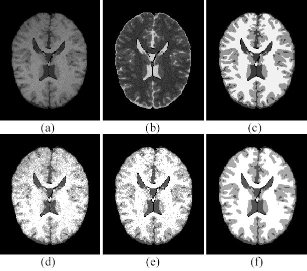
Digital phantom studies. (a) T₁ weighted image. (b) T₂ weighted image. (c) The ground truth of hard segmentation. (d) The FCM segmentation. (e) The AFCM segmentation. (f) The presented PV-MAP segmentation.

Figure 1(c) is the ground truth of hard segmentation. The PV segmentation results of different algorithms were obtained first and then converted into hard segmentations, respectively, for comparison purpose. The conversion labels a voxel by a tissue type, which has the largest mixture percentage among all the tissue types in that voxel. Figure 1(d) is the hard segmentation converted from the FCM segmentation result. Because of the inhomogeneity effect, the WM is missed at the top region and over-segmented at the bottom area. Figures 1(e) and 1(f) show the hard segmentation results converted from the AFCM and our PV-MAP segmentations, respectively. Both methods can correct for the inhomogeneity effect very well. However, there are many speckles in the AFCM segmentation due to the presence of noise. By visual judgment, our method has a better performance against noise compared with the AFCM result. For a more objective comparison among the FCM, AFCM and our method, a quantitative analysis of the whole 3D image volume was conducted. Table I shows the quantitative results of different methods based on the TPF, FPF and ASR measures. In the presence of noise and the inhmonogenity effect, the ASR value of the FCM algorithm is very low (75.16%), which is not acceptable in the clinic. Because the AFCM algorithm takes into account the inhomogeneity effect, its ASR value can be improved to 82.60%. An improvement in TPF and FPF is also noticeable. It is notable that the presented method can achieve an ASR value of 91.49% and improve TPF and FPF for all tissue types.

TABLE I.

QUANTITATIVE COMPARISON OF FCM, AFCM AND PV-MAP METHODS (%).

	FCM			AFCM			PV-MAP
	WM	GM	CSF	WM	GM	CSF	WM	GM	CSF
TPF	74.57	73.60	80.69	76.58	85.80	93.26	91.96	90.27	93.96
FPF	21.42	31.66	15.63	7.58	31.08	12.95	6.94	9.08	10.92
ASR	75.16			82.60			91.49

Figure 2 shows the segmented mixture images of different tissue types obtained using different segmentation methods. Figures 2(a), 2(b) and 2(c) are the true mixture models of CSF, GM and WM, respectively. Figures 2(d), 2(e) and 2(f) show the mixture images of CSF, GM and WM obtained with the FCM algorithm. It is noted that there are severe shading artifacts on the GM and WM mixtures because the FCM did not correct for the image intensity inhomogeneity. This shading effect is completely removed by the AFCM and PV-MAP method, as shown in Figures 2(g)–2(l). However, segmented mixture images obtained via the AFCM method demonstrate a weak performance against noise. By including the MRF model into the presented PV-MAP framework, our segmentation scheme overcomes not only the inhomogeneity effect but also the noise effect.

Figure 2.

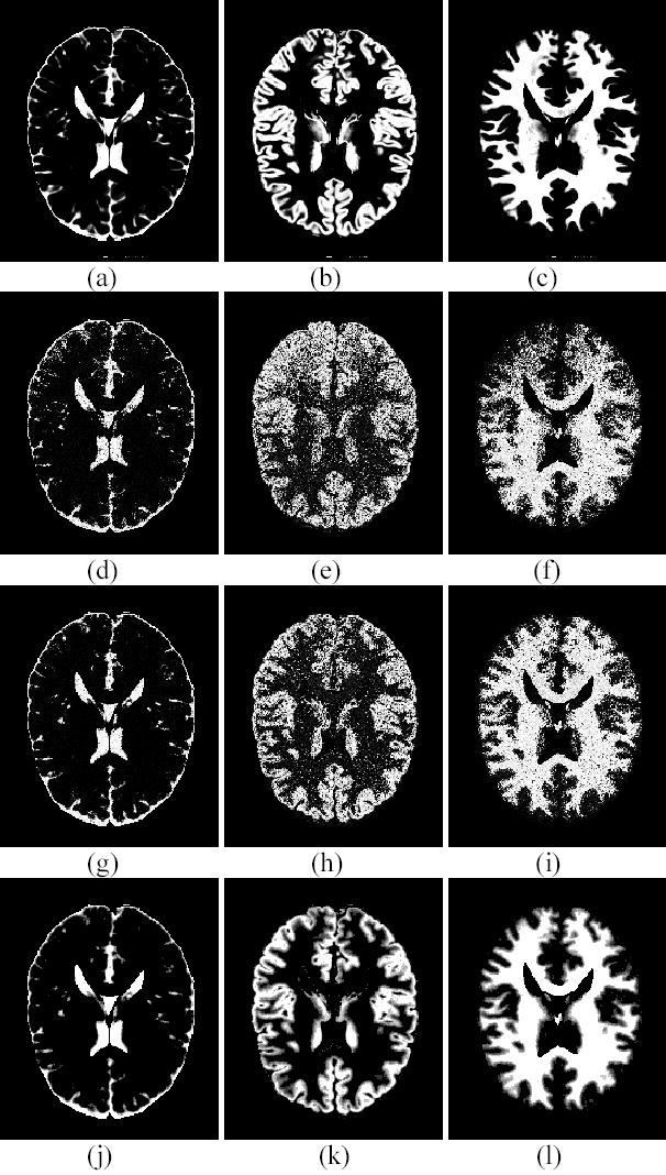
Comparison on segmented mixture images. (a) The true model of CSF mixture. (b) The true model of GM mixture. (c) The true model of WM mixture. (d) The segmented CSF mixture by FCM. (e) The segmented GM mixture by FCM. (f) The segmented WM mixture by FCM. (g) The CSF mixture by AFCM. (h) The GM mixture by AFCM. (i) The WM mixture by AFCM. (j) The CSF mixture of PV-MAP. (k) The GM mixture of PV-MAP. (l) The WM mixture of PV-MAP.

The presented PV-MAP method has three parameters, α, λ₁ and λ₂, to be specified, as shown in equation (10). For a penalized estimation algorithm, the robustness of these parameters is a very important issue. In reference [7], the robustness of parameters λ₁ and λ₂ has been studied. Based on their work⁷, λ₁ and λ₂ were determined to be 40000 and 400000, respectively. The value of parameter α is empirically defined as follows:

$$\alpha =\xi \frac{{({\upsilon }_{T1WM}-{\upsilon }_{T1CSF})}^2}{8}$$ (24)

where υ_T1WM and υ_T1CSF are the centroids of WM and CSF in T₁-weighted MR images, respectively. In general, ζ equals one. In order to investigate the influence of the parameter α on the performance of the presented segmentation method, we have selected ζ to be different values: 0.1, 0.2, 0.4, 0.6, 0.8, 1, 2, 4, 6, 8, 10 and repeated the above segmentation procedure to obtain the corresponding ASR values. Figure 3 demonstrates the relationship between ζ and ASR. Over a large range of α values (where ζ value varies from 0.4 to 8), the ASR of the PV-MAP method is greater than 0.91. For all of these ζ values, the performance of the new method is better than the AFCM algorithm (which has an ASR value of 0.83).

Figure 3.

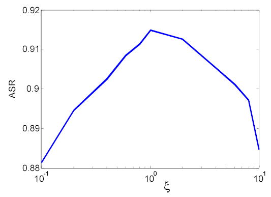
Robustness study of the parameter α.

B. Clinical data studies

MRI sessions were conducted using a 1.5Tesla Phillip Edge whole-body scanner with a body coil as the transmitter and a birdcage head coil as the receiver. 3D SPGR and 3D EXPRESS sequences were employed to acquire T₁ and T₂ weighted axial images covering the whole brain with 30° flip angle, 1.5 mm slice thickness, 24 cm FOV, and 256×256 matrix size (0.9375 by 0.9375 mm). For the T₁ weighted image, T_R=50 ms, T_E=5 ms. For the T₂ weighted image, T_R = 4000 ms, T_E = 95 ms.

The self-adaptive vector quantization method³⁰ was used to first remove the skull and scalp and generate the initial centroids for each class. Next, the whole brain volume was segmented into three classes: WM, GM and CSF. Figures 4(a) and 4(b) show a slice of the T₁ and T₂ weighted volume images after the preprocessing above, respectively. Figures 4(c), 4(d) and 4(e) show the segmentation results of the same slice using the FCM, AFCM and PV-MAP method, respectively. It is noted that the FCM segmentation result is affected severely by the noise and inhomogeneity effect. The central WM area contains many small spots. The regions of interest (ROIs) indicated by the arrows near the FOV edge show the errors, which are mainly due to the inhomogeneity effect. The AFCM improved upon the results of FCM noticeably because of its correcting for the inhomogeneity effect. However, like the FCM, the AFCM is not able to overcome the noise effect, because neither of them includes the MRF model for noise control. On the other hand, the presented PV-MAP method demonstrates robustness against noise as shown in Figure 4(e). It also achieves excellent performance in correcting for the inhomogeneity effect with the corresponding bias field estimation as shown in Figure 4(f). Unlike the phantom studies, we do not have a gold standard for comparison in clinical studies. All of the comparisons are based on visual judgment. Most importantly, these experimental results concur with the theoretical predictions by the PV-MAP framework, which considers noise, PV effect, image inhomogeneity, and multi-spectral characteristics simultaneously.

Figure 4.

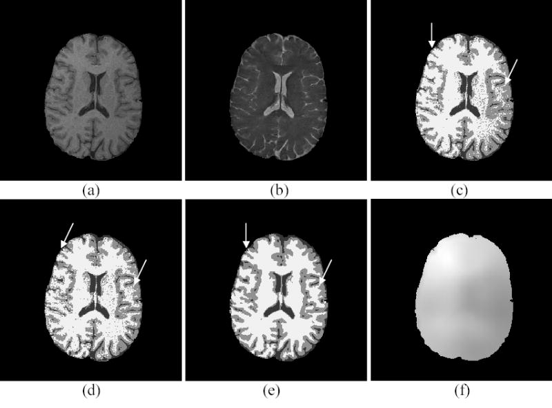
Clinical study. (a) T₁ weighted image. (b) T₂ weighted image. (c) The FCM segmentation. (d) The AFCM segmentation. (e) The PV-MAP segmentation. (f) The bias field estimated by the PV-MAP segmentation method.

IV. Discussion

Our PV-MAP method encompasses the well-known FCM and AFCM algorithms. This can be shown from the posterior energy function U described in equations (4) and (10). When α is set to zero, the proposed method reduces to the AFCM algorithm. If the bias field B is further confined to be a constant value of one, the AFCM further reduces to the FCM. The FCM reflects only the likelihood energy function in the MAP framework and the AFCM incorporates only the prior probability of the bias field B into the FCM. Neither FCM nor AFCM algorithms take into account the prior information of the mixture M, thus they fail to obtain good segmentation results for noisy MR images, which is inadequate for analysis of noisy clinic studies.

There are many ways to deal with the noise in the MR images. Edge-preserving noise filtering by an anisotropic diffusion filter (ADF) is one of many choices^32,33. By this approach, segmenting a noisy brain MR image is performed by first smoothing the image with the ADF and then applying a previously developed segmentation method (such as the FCM or AFCM or others^34,35) to the smoothed image. If the noise can be effectively filtered, i.e., the noise-free image can be estimated from the noisy one, most of the previous segmentation methods shall work well. To the best of our knowledge, most edge-preserving filters are suitable for the piecewise images. When there exist strong inhomogeneity or partial volume effects, the noisy images are not piecewise images anymore. The drawback of this noise-filtering and then image-segmentation approach is that a possible inconsistence of the segmented result with the original image data may occur³⁶. To realize this, we performed another study. The 3D MR images with 5% noise level and different inhomogeneity effects were used. The FCM or AFCM algorithm was applied to the filtered image by the ADF. Table II shows the quantitative assessment results without inhomogeneity effect and Table III shows the results with 60% inhomogeneity effect. From these experimental results, we found that without inhomogeneity effect, FCM plus ADF approach can achieve a similar performance for noise reduction as the PV-MAP method. In the presence of inhomogeneity effect, AFCM plus ADF also showed improvement. As shown in Table I, compared with the result of AFCM algorithm, the approach of ADF filtering plus AFCM segmentation improves the ASR accuracy from 82.60% to 86.07%. However, its performance degrades in the presence of imhomogeneity effect compared with our proposed method. Therefore, the advantage of the proposed method is that it models all the effects, aiming to obtain an unbiased estimate of the noise-free signal consistent with the measured noisy data³⁶.

TABLE II.

QUANTITATIVE ASSESSMENT OF ADF FILTERING ON NOISY IMAGE WITHOUT INHOMOGENEITY EFFECT (%)

	FCM			PV-MAP			FCM+ADF
	WM	GM	CSF	WM	GM	CSF	WM	GM	CSF
TPF	96.03	91.18	95.12	96.87	93.94	94.21	96.63	93.43	93.95
FPF	9.25	4.98	4.63	5.89	4.72	4.02	6.26	5.01	4.58
ASR	93.60			95.01			94.64

TABLE III.

QUANTITATIVE ASSESSMENT OF ADF FILTERING ON NOISY IMAGE WITHOUT INHOMOGENEITY EFFECT (%)

	ADF+AFCM
	WM	GM	CSF
TPF	97.15	78.67	89.16
FPF	25.53	6.59	5.50
ASR	86.07

In our PV-MAP framework, the definitions of the prior probabilities of mixture M of equation (5), and bias field B of equation (7) are not unique. For example, alternate mixture prior models for equation (5) were reported in references [10–12]. Comparing these prior models would be an interesting research topic and is under progress. For the bias field model of equation (7), many linear filter H can be used to model the banded covariance matrix ∑_B in equation (7). Furthermore instead of using the Jacobian iterative scheme, the estimation of the bias field in equation (18) could be implemented by the following scheme^23,24:

$${\beta }_i=\frac{{[f(Q)]}_i}{{[f(A)]}_i}$$ (25)

where f represents the low-pass filter, which corresponds to the prior model of bias field B, and Q and A were defined in equation (18). The Jacobian iterative scheme with multi-grid strategy was employed due to its improved computational efficiency. For 3D digital MR phantom data with 181×217×181 size, the total calculation time was about 10 minutes on a 2.4 GHz Pentium IV PC with 1Gbyte memory. It is noted that equation (17) appears to be close to a discrete Poisson equation. There are highly developed analytic solutions³⁷ which will dramatically increase the computational efficiency for solving such equation. We will investigate the analytic solutions for an efficiency estimation of the bias field in our future work.

In this paper, the extended FCM equation was used to model the likelihood energy function U (Y M, B,Φ) of equation (4). An alternative likelihood energy function could be the PV Gaussian mixture model^10–12. One reason for choosing the extended FCM model in this paper is that the estimation of parameter Φ can be easily obtained by directly maximizing the posterior energy function as defined in equation (10). If the Gaussian mixture model^10–12 is considered, there are two problems that need to be solved. First, the extended Gaussian mixture model with correction of the inhomogeneity effect would need to be developed. Second, the estimation of parameter Φ for the Gaussian mixture model is not trivial and can be very difficult as compared to a conventional hard segmentation method (e.g., the MRF-EM framework^2,38). Research on these two problems is currently under investigation by our group^12,39.

In the work of Leemput et al¹¹, the PV effect was modeled by a down-sampling process, which means that PV effect comes from insufficient special resolution of the imaging devices and remains only in the boundary region between different tissues, and Monte-Carlo method was used to label the sub-voxels in each of the original image voxel. Their method has shown good performance of solving the PV effect. However, their method may not solve the case, in which the GM and WM are truly mixed without interfaces, as mentioned in their paper. This phenomenon occurs more often inside the tissues, which may have a pathological change, and is a very important feature for patient diagnosis. We call such segmentation as mixture segmentation, which is a more general concept than the PV segmentation. Therefore, the solution for mixture segmentation should be preformed in the continuous spaces. Accurate prior information on the mixture M is required, especially for images with more tissue types. Further investigation on this topic is one of our future research interests^12,39.

Finally, it should be pointed out that our PV-MAP method has some limitations. The choice of weighting parameters α, λ₁ and λ₂ is empirical. In addition, the minimization algorithm used in this paper is one type of conjugate gradient method and cannot promise to converge to the global minimum, although a lot of experiments have demonstrated that it always converges to a satisfactory result. Further theoretical research is needed. The simulated annealing method or genetic algorithm may be the solution²⁵.

V. Conclusion

A PV-MAP framework for brain MR image segmentation was proposed. The presented approach has taken into account the inherent effects of brain MR imaging including: noise, PV effect, image-intensity inhomogeneity and multi-spectral characteristics simultaneously. This framework has theoretically summarized the current FCM-based segmentation methods. Digital phantom and clinical patient data studies demonstrate that this framework can improve segmentation performance than the AFCM algorithm in the presence of noise, PV effect and intensity inhomogeneity, which are commonly encountered in clinic studies.

References

- 1.Vannier M, Butterfield R, Jordon D, Murphy W, Levitt RG, Gado M. “Multi-spectral analysis of magnetic resonance images,”. Radiology. 1985;154:221–224. doi: 10.1148/radiology.154.1.3964938. [DOI] [PubMed] [Google Scholar]
- 2.Liang Z, MacFall JR, Harrington DP. “Parameter estimation and tissue segmentation from multispectral MR images,”. IEEE Trans Medical Imaging. 1994;13:441–449. doi: 10.1109/42.310875. [DOI] [PubMed] [Google Scholar]
- 3.Rajapakse JC, Giedd JN, Rapoport JL. “Statistical approach to segmentation of single channel cerebral MR images,”. IEEE Trans Medical Imaging. 1997;16:176–186. doi: 10.1109/42.563663. [DOI] [PubMed] [Google Scholar]
- 4.Zhang Y, Brady M, Smith S. “Segmentation of brain MR images through a hidden Markov random field model and expectation-maximization algorithm,”. IEEE Trans Medical Imaging. 2001;20:45–57. doi: 10.1109/42.906424. [DOI] [PubMed] [Google Scholar]
- 5.Leemput KV, Maes F, Vandermeulen D, Colchester A, Suetens P. “Automatic segmentation of multiple sclerosis lesion by model outlier detection,”. IEEE Trans Medical Imaging. 2001;20:677–688. doi: 10.1109/42.938237. [DOI] [PubMed] [Google Scholar]
- 6.Pham DL, Prince JL. “An adaptive fuzzy C-means algorithm for image segmentation in the presence of intensity inhomogeneities,”. Pattern Recognition Letters. 1999;20:57–68. [Google Scholar]
- 7.Pham DL, Prince JL. “Adaptive fuzzy segmentation of magnetic resonance images,”. IEEE Trans Medical Imaging. 1999;18:737–752. doi: 10.1109/42.802752. [DOI] [PubMed] [Google Scholar]
- 8.Ahmed MN, Yamany SM, Mohamed N, Farag AA. “A modified fuzzy C-mean algorithm for bias field estimation and segmentation of MRI data,”. IEEE Trans Medical Imaging. 2002;21:193–199. doi: 10.1109/42.996338. [DOI] [PubMed] [Google Scholar]
- 9.Li X, Li L, Lu H, Chen D, Liang Z. “Inhomogeneity correction for magnetic resonance images with fuzzy C-mean algorithm,”. Proceedings of SPIE Medical Imaging. 2003;5032:995–1005. [Google Scholar]
- 10.Choi HS, Haynor DR, Kim Y. “Partial volume tissue classification of multi-channel magnetic resonance images- A mixel model,”. IEEE Trans Medical Imaging. 1991;10:395–407. doi: 10.1109/42.97590. [DOI] [PubMed] [Google Scholar]
- 11.Van Leemput K, Maes F, Vandermeulen D, Suetens P. “A unifying framework for partial volume segmentation of brain MR images,”. IEEE Trans Medical Imaging. 2003;22:105–119. doi: 10.1109/TMI.2002.806587. [DOI] [PubMed] [Google Scholar]
- 12.X. Li, D. Eremina, L. Li, and Z. Liang, “Partial volume segmentation of medical images,” Conference Record of IEEE NSS-MIC, in CD-ROM, 2003.
- 13.Axel L, Costantini J, Listerud J. “Intensity correction in surface coil MR imaging,”. American Journal of Roentgenology. 1987;148:418–420. doi: 10.2214/ajr.148.2.418. [DOI] [PubMed] [Google Scholar]
- 14.Foo TKF, Hayes CE, Kang YW. “Reduction of RF penetration effects in high field imaging,”. Magnetic Resonance in Medicine. 1992;23:287–301. doi: 10.1002/mrm.1910230209. [DOI] [PubMed] [Google Scholar]
- 15.Dawant BM, Zijidenbos AP, Margolin RA. “Correction of intensity variation in MR images for computer-aided tissue classification,”. IEEE Trans Medical Imaging. 1993;12:770–781. doi: 10.1109/42.251128. [DOI] [PubMed] [Google Scholar]
- 16.Lim KO, Pfefferbaum A. “Segmentation of MR brain images into cerebrospinal fluid and white and gray matter,”. J Comput Assisted Tomography. 1989;13:588–593. doi: 10.1097/00004728-198907000-00006. [DOI] [PubMed] [Google Scholar]
- 17.Johnstion B, Atkins MS, Mackiewich B, Anderson M. “Segmentation of multiple sclerosis lesions in intensity corrected multi-spectral MRI,”. IEEE Trans Medical Imaging. 1996;15:154–169. doi: 10.1109/42.491417. [DOI] [PubMed] [Google Scholar]
- 18.Liang Z, Wang D, Ye J, Li H, Roque C, Harrington D. “Correction of RF Inhomogeneity for Automatic Segmentation from Multi-spectral MR Images,”. Proceedings of International Society of Magnetic Resonance in Medicine. 1997;3:p.2042. [Google Scholar]
- 19.Brinkman BH, Manduca A, Robb RA. “Optimized homomorphic unsharp masking for MR grayscale inhomogeneity correction,”. IEEE Trans Medical Imaging. 1998;17:161–171. doi: 10.1109/42.700729. [DOI] [PubMed] [Google Scholar]
- 20.Vokurka EA, Thacker NA, Jackson A. “A fast model independent method for automatic correction of intensity non-uniformity in MRI data,”. J Magnetic Resonance Imaging. 1999;10:550–562. doi: 10.1002/(sici)1522-2586(199910)10:4<550::aid-jmri8>3.0.co;2-q. [DOI] [PubMed] [Google Scholar]
- 21.Lee SK, Vannier MW. “Post-acquisition correction of MR inhomogeneity,”. Magnetic Resonance in Medicine. 1996;36:275–286. doi: 10.1002/mrm.1910360215. [DOI] [PubMed] [Google Scholar]
- 22.Chen D, Li L, Yoon D, Lee J, Liang Z. “A renormalization method for inhomogeneity correction of MR images,”. Proceeding of SPIE Medical Imaging. 2001;4322:939–942. [Google Scholar]
- 23.Wells WM, Grimson WEL, Kikinis R, Jolesz FA. “Adaptive segmentation of MRI data,”. IEEE Trans Medical Imaging. 1996;15:429–442. doi: 10.1109/42.511747. [DOI] [PubMed] [Google Scholar]
- 24.Guillemaud R, Brady M. “Estimating the bias field of MR images,”. IEEE Trans Medical Imaging. 1998;16:238–251. doi: 10.1109/42.585758. [DOI] [PubMed] [Google Scholar]
- 25.Held K, Kops ER, Krause BJ, Wells WM, Kikinis R, Müller-Gärtner HW. “Markov random field segmentation of brain MR images,”. IEEE Trans Medical Imaging. 1997;16:878–886. doi: 10.1109/42.650883. [DOI] [PubMed] [Google Scholar]
- 26.T. Kapur, W.E.L. Grimson, R. Kikinis and W.M. Wells, “Enhanced spatial priors for segmentation of magnetic resonance imaging,” in Lecture Notes in Computer Science. Proceedings of Medical Image Computing and Computer-Assisted Intervention-MICCAI’98, p.457–468, 1998.
- 27.K.M. Pohl, W.M. Wells, A. Guimond, K. Kasai, M.E. Shenton, R. Kikinis, W.E.L. Grimson and S.K. Warfield. “Incorporating non-rigid registration into expectation maximization algorithm to segment MR images,” in Lecture Notes in Computer Science. Proceedings of Medical Image Computing and Computer-Assisted Intervention-MICCAI’02, p.457–468, 2002. [DOI] [PMC free article] [PubMed]
- 28.P. Wesseling, An Introduction to Multigrid Mthods, Wiley, New York, pp. 42, 1992.
- 29.Unser M. “Multigrid adaptive image processing,”. Proceedings of IEEE Conference on Image Processing. 1995;I:49–52. [Google Scholar]
- 30.Chen D, Li L, Liang Z. “A self-adaptive vector quantization algorithm for MR image segmentation,”. Proceedings of International Society of Magnetic Resonance in Medicine. 1999;1:p.122. [Google Scholar]
- 31.Cocosco CA, Kollokian V, Kwan RKS, Evans AC. “BrainWeb: Online interface to a 3D MRI simulated brain database,”. NeuroImage. 1997;5(4):S425. http://www.bic.mni.mcgill.ca/brainweb/. [Google Scholar]
- 32.Gerig G, Kübler O, Kikinis R, Jolesz F. “Nonlinear anisotropic filtering of MRI data,”. IEEE Trans Medical Imaging. 1992;11:221–232. doi: 10.1109/42.141646. [DOI] [PubMed] [Google Scholar]
- 33.Winkler G, Aurich V, Hahn K, et al. “Noise reduction in images: Some recent edge-preserving methods,”. Pattern Recognition and Image Analysis. 1999;9(4):749–766. [Google Scholar]
- 34.Zeng X, Staib LH, Schultz RT, Duncan JS. “Segmentation and measurement of the cortex from 3-D MR images using coupled- surfaces propagation,”. IEEE Trans Medical Imaging. 1999;18:927–937. doi: 10.1109/42.811276. [DOI] [PubMed] [Google Scholar]
- 35.Grau V, Mewes AUJ, Alcayiz M, Kikinis R, Warfield SK. “Improved watershed transform for medical image segmentation using prior information,”. IEEE Trans Medical Imaging. 2004;23:447–458. doi: 10.1109/TMI.2004.824224. [DOI] [PubMed] [Google Scholar]
- 36.Wang J, Lu H, Li T, Liang Z. “Sinogram noise reduction for low-dose CT by statistics-based nonlinear filters”. Proceedings of SPIE Medical Imaging. 2005;5747 to appear. [Google Scholar]
- 37.Hu GY, Ryu JY, O’Conell RF. “Analytical solution of the generalized discrete poisson equation,”. J Phys A: MathGen. 1998;31:9279–9282. [Google Scholar]
- 38.Dempster A, Laird N, Rubin D. “Maximum likelihood from incomplete data via the EM algorithm,”. J R Stat Soc. 1977;39B:1–38. [Google Scholar]
- 39.Liang Z, Li X, Eremina D, Li L. “An EM framework for segmentation of tissue mixtures from medical images”. Proceedings of International Conference of IEEE Engineering in Medicine and Biology, Concun, Mexico. 2003:682–685. [Google Scholar]