On atomic force microscopy and the constitutive behavior of living cells

Abstract

Atomic force microscopy (AFM) is one of many new technologies available to study the mechanical properties and mechanobiological responses of living cells. Despite the widespread usage of this technology, there has been little attempt to develop new theoretical frameworks to interpret the associated data. Rather, most analyses rely on the classical Hertz solution for the indentation of an elastic half-space within the context of linearized elasticity. In contrast, we propose a fully nonlinear, constrained mixture model for adherent cells that allows one to account separately for the contributions of the three primary structural constituents of the cytoskeleton. Moreover, we extend a prior solution for a small indentation superimposed on a finite equibiaxial extension by incorporating in this mixture model for the special case of an initially random distribution of constituents (actin, intermediate filaments, and microtubules). We submit that this theoretical framework will allow an improved interpretation of indentation force–depth data from a sub-class of atomic force microscopy tests and will serve as an important analytical check for future finite element models. The latter will be necessary to exploit further the capabilities of both atomic force microscopy and nonlinear mixture theories for cell behavior.

Introduction

Among the myriad of exciting discoveries of modern biology is the observation that many types of cells respond dramatically to changes in their mechanical environment. Such cells may alter their orientation, shape, internal constitution, contraction, migration, adhesion, synthesis and degradation of extracellular constituents, or even their life cycle in response to perturbations in mechanical loading (Zhu et al. 2000). Counted among these cell types are the chondrocytes, endothelial cells, epithelial cells, fibroblasts, macrophages, myocytes, and osteocytes, to name but a few. Although much has been learned about the mechanosensitive responses of living cells, there remains a pressing need for quantification and, in particular, for mathematically modeling the mechanobiology (Fung 2002).

Atomic force microscopy (AFM) is one of several new technologies that promise to increase our understanding of the mechanobiology and biomechanics of living cells (Radmacher et al. 1992). Briefly, the AFM is a cantilever-based scanning probe that can be operated in two primary modes: the constant force mode allows the AFM to serve as a highly sensitive profilometer, thus, enabling one to map the surface topography of a cell (Fig. 1); the displacement mode allows one to perform mechanical tests on cells, in particular, local indentation or local pulling following adhesion of the probe. The tip of the cantilever largely dictates the resolution and “sphere of influence” of the mechanical interrogation. Tips can be microfabricated to have different sizes and shapes, but many are on the order of 10–50 nm and shaped either as a cone or a blunted-cone with a spherical cap. In the displacement mode, common indentations are on the order of 50–500 nm, with the thickness of the cell often on the order of 1–3 μm.

Fig. 1.

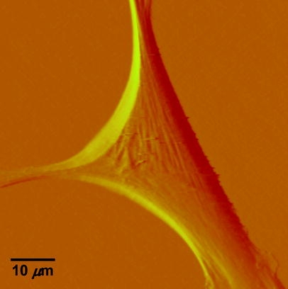
Deflection image of a vascular smooth muscle cell isolated from the rat skeletal muscle arterioles. The AFM probe was scanned across the cell surfaces at a speed of 40 µm/s, with a tracking force of approximately 400 pN. The image was collected using Nanoscope IIIa Software

Most AFM-based studies of the mechanical behavior of living cells (e.g., Wu et al. 1998; Rotsch and Radmacher 2000; Mathur et al. 2001) are interpreted using the classical Hertz solution for the indentation of an elastic half-space (e.g., Sneddon 1965). This solution was derived, of course, within the context of the many simplifying assumptions of classical elasticity: linear elastic behavior, material uniformity and homogeneity, isotropy, and infinitesimal strains. Few of these assumptions apply to living cells or the associated test conditions (Costa and Yin 1999). Rather, cells are materially nonuniform, consisting of multiple families of structurally important and highly organized proteins that may exhibit a nonlinear behavior over finite deformations (e.g., see Janmey et al. 1991; Liu and Pollack 2002). The purpose of this paper, therefore, is twofold: to present a new nonlinear constitutive model for cells that accounts for their inherent material non-uniformity as well as potential material and geometric nonlinearities, and to extend a prior solution from the finite elasticity literature for use in a sub-class of AFM studies of cell mechanics. In particular, we submit that a constrained mixture model of the cytoskeleton offers potential advantages over many prior models, since one can account for constituent-specific changes in mechanical properties that have been reported recently in AFM studies (e.g., Wu et al. 1998; Rotsch and Radmacher 2000).

Background

Constrained mixture models

Adherent cells consist of three primary components: the cell membrane, cytoplasm, and nucleus. Whereas a complete description of cell mechanics will require separate descriptions of the mechanical properties of each component, here, we consider a homogenized idealization that holds away from the nucleus and in cases of negligible bending stiffness of the membrane. The cytoplasm consists of a viscous fluid (called the cytosol), distributed organelles, and the cytoskeleton. The cytoskeleton endows the cell with most of its structural integrity and consists of three primary constituents: actin filaments, intermediate filaments, and microtubules. These filaments are on the order of 5–25 nm in diameter and are often distributed throughout the cytoplasm. Although one could employ a full mixture theory (see Rajagopal and Tao 1995) to describe the mechanics of such a multi-constituent material, which would require the solution of separate balance relations for the constituents, there is a lack of information on the interactions between the three primary constituents as well as between these constituents and the many accessory proteins (Alberts et al. 2002). Thus, it is not possible at present to postulate the constitutive relations for momentum exchanges between constituents that are needed in a full mixture theory. Following Humphrey (2002a), therefore, we adopt a homogenized rule-of-mixtures model for the stress response. This allows us to include the separate contributions of the primary cytoskeletal filaments and viscous cytosol without having to solve separate balance relations for each constituent, to quantify the momentum exchanges, or to prescribe partial traction boundary conditions. A general rule-of-mixtures relation for the total Cauchy stress t (subject to an overall linear momentum balance) can be written as , where φ^k are individual mass fractions and t^k are the individual stress responses, whether elastic or viscous. Indeed, including both the “elastic” response of the filaments and the “viscous” response of the cytosol may allow one to model some of the complex viscoelastic responses exhibited by cells (e.g., see Heidemann et al. 1999).

For motivational purposes, let us also consider a simple case wherein any mechano-sensitive changes in the polymerization or depolymerization of the structural filaments occur in but a single altered (i.e., new) configuration. In this case, one must track constituents that existed prior to the perturbation in loading (original) plus those produced thereafter (new). Within the context of a rule-of-mixtures approach, the associated stress response can be written as (Humphrey 2002a):

1

where p is a Lagrange multiplier that enforces incompressibility over transient loading, D is the stretching tensor (i.e., where the over-dot denotes a time-derivative), is a viscosity, the F_κ are deformation gradient tensors for each constituent relative to individual natural configurations κ_o (original) or κ_n (new), and the φs are mass fractions (i.e., constituent mass per total mass) of individual constituents, which, by definition, are subject to the constraint:

2

Specifically, the subscript o denotes “original” and n denotes “new” whereas the superscripts c, a, i, and m denote cytosol, actin, intermediate filaments, and microtubules, respectively. In other words, we assume that the stress response depends both on the response of extant constituents that formed prior to any perturbation in loading as well as on constituents that formed thereafter. (Note: although some constituents turn over continuously, there is no net change in mass fraction or mechanical behavior when they do so equally in an unchanging configuration, which we refer to as maintenance.) In the absence of turnover in an altered configuration, the mass fractions of the new constituents are zero, thus yielding the standard rule-of-mixtures relation for stress.

Finally, note that the assumption of a constrained mixture requires that constituents deform together; because these constituents may have different natural (i.e., stress-free) configurations, the individual deformation gradients F_κ need not be the same. Similarly, the individual stress responses t^k are expected to differ (k = a, i, m for actin, intermediate filaments, and microtubules, respectively). Indeed, this is one of the primary advantages of a mixture theory. Nevertheless, we emphasize that, in such a formulation, the t^k represent “constituent-dominated” phenomenological responses that implicitly include constituent-to-constituent interactions that cannot be quantified in sufficient detail (see Brodland and Gordon 1990). See Humphrey (2002a) for more details on the basic theory.

Lessons from finite elasticity

It has been well known for nearly a century that biological soft tissues and elastomeric materials share many characteristic behaviors (see Treloar 1975; Humphrey 2002b). This similarity results largely from both classes of materials exhibiting primarily an entropic, not energetic, elasticity due to their underlying long chain polymeric microstructures. Consequently, many results from finite (rubber) elasticity can be very useful in biomechanics. One solution that is particularly relevant to some AFM studies is that of a small, quasi-static indentation superimposed on a finite equibiaxial stretch of an initially isotropic, nonlinearly elastic, materially uniform, incompressible material whose behavior is described by a strain-energy function W=W(I₁, I₂). Briefly, the associated constitutive relation for the Cauchy stress is:

3

where B=FF^T is the left Cauchy–Green tensor and I₁=trC and 2I₂= (trC)²−trC² are the principal invariants of the right Cauchy–Green tensor C=F^TF. For an initial, finite equibiaxial stretch, we let F=diag[μ, μ, λ], where μ is the in-plane stretch and λ is the out-of-plane stretch; by incompressibility, λ=1/μ², thus, allowing the deformation to be parameterized by one stretch. For completeness, let us summarize past results for the small, superimposed indentation.

The superimposed indentation force–depth (P–δ) relationship was found by Green et al. (1952) and Beatty and Usmani (1975). It can be written as:

4

where Γ(W) and Σ(W) are functionals that depend on the strain-energy function W and the finite equibiaxial stretch μ, whereas the function depends on the geometry of the tip of the rigid indenter. For example, Costa and Yin (1999) list the following results for different tip geometries. For a flat-ended circular indenter of radius a:

5

for a spherical tip of radius a:

6

for a conical tip with tip angle 2Φ:

7

and for a blunted cone-shaped tip of angle 2Φ, which transitions at radius b to a spherical cap of radius a:

8

where the radius of contact r_c≥b and is obtained from Eq. 9, namely (Briscoe et al. 1994)

9

Finally, Humphrey et al. (1991) list the following results for computing Γ(W) and Σ(W):

10

where

11

and K₁ and K₂ (dimensionless) are determined by solving the following quadratic equation for K:

12

with

13

and

14

Note that, for convenience, we denote:

15

Together, Eqs. 4–15 allow one to compute the indentation force–depth relation for an incompressible, initially isotropic material that is first stretched equibiaxially (note: this stretch induces an anisotropy relative to the original reference configuration). In the next section, we extend this result for a special case of a new relationship for cell mechanics that accounts for the separate contributions of the three primary cytoskeletal constituents.

New theoretical framework

A constitutive relation for cells

Many different models have been proposed for the constitutive behavior of cells (e.g., see Humphrey 2002a; Stamenovic and Ingber 2002). These include tensegrity models, percolation models, soft glassy rheological models, mixture models, and classical models based on linearized elasticity or viscoelasticity. Notwithstanding the potential advantages of the different models, we submit that constrained rule-of-mixture models (see Eq. 1) allow one to include nonlinear elasticity and viscoelasticity, different properties and distributions of individual constituents, and, most importantly, the different rates and extents of turnover of individual constituents. Here, therefore, consider the following relation for the Cauchy stress:

16

where the viscosity may depend on the mass fraction of the cytosol. That is, as insoluble constituents are depolymerized, their fragments may alter the viscosity (see Herant et al. 2003). More important here, however, we borrow from the work of Lanir (1983) to construct a strain-energy function for a potentially evolving cytoskeleton, while emphasizing that the resulting relations are microstructurally-motivated, but phenomenological, namely:

17

where w^k(α^k) is a 1-D strain energy function for a filament and α^k is its stretch; the superscript k can denote a particular constituent as well as its natural configuration (e.g., original vs. new). The function R^k(ϕθ) represents the original distribution of orientations of a filament family k and ^k are mass fractions. Consequently:

18

where the 1′ (i.e., primed) coordinate axis coincides with the direction of a generic filament (Fig. 2), and is obtained from a tensorial transformation of C_MN. This relation will prove useful below. Hence, we have:

19

Clearly then, in the absence of constituent turnover, our constitutive relation can be written as a simple rule-of-mixtures with each primary constituent having a single reference configuration (i.e., N=1, 2, 3 for original actin a, intermediate filaments i, and microtubules m), namely:

20

Turnover of constituents can easily be incorporated in Eq. 19, in principle, given appropriate kinetics for the mass fractions, information on the potential evolution of the individual natural configurations, and information on the potential evolution of the distribution of the filaments. This is left for subsequent consideration.

Fig. 2.

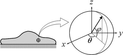
Local spherical coordinate system used for microstructurally motivated, phenomenological constitutive relations of a living cell. The arrow represents the orientation of an individual filament belonging to any of the three primary families of cytoskeletal filaments. The function R^k(ϕ, θ) quantifies the distribution of all such orientations

Small indentation superimposed on a finite equibiaxial stretch

Conceptually, it may be prudent to think of at least four configurations for the cell in an AFM test (Fig. 3). First, we have a non-adherent cell with perhaps a fairly random distribution of cytoskeletal filaments. Deposition of the cell onto a substrate involves two phases: initial contact, with an upregulation of integrins, followed by an active spreading. Relative to the non-adherent reference configuration, we might think of this spreading as somewhat of an in-plane stretch. Finally, if the substrate is deformable, the cell could be stretched further prior to testing with the AFM. This potential sequence of events motivates the consideration of a small indentation superimposed on a large “in-plane” deformation of a mixture that originally had a nearly uniform distribution of constituents. Whereas the aforementioned solution for the relation P–δ (Eq. 4) was derived for a 3-D stored energy function W(I₁, I₂), the proposed strain-energy for the cell (Eq. 17) is written in terms of individual 1-D stored energy functions w^k that depend solely on the stretch α^k experienced by the individual constituent. Fortunately, these stretches relate to the macroscopic deformation C, if we assume affine deformations. Hence, we merely need transformation relations between derivatives with respect to the invariants I_i and those in terms of the components of C in order to utilize prior results for the indentation solution. Note, therefore, that:

21

whereby, for an in-plane equibiaxial stretch, we need only to consider derivatives with respect to C₁₁, C₂₂, and C₃₃. These provide three equations in terms of the two “unknown” derivatives of W with respect to I₁ and I₂, which are denoted by W₁ and W₂, respectively. For an equibiaxial stretch, however, the results for the in-plane components C₁₁ and C₂₂ are the same and it is easy to show that:

22

23

Next, let and consider the following derivatives:

24

which provide six equations in terms of the four “unknown” second derivatives of W with respect to the invariants, which we denote by W_ij=W_ji (see Eq. 15). As before, however, the equations for the components C₁₁ and C₂₂ provide the same information, thus leaving four equations. Solving these four equations for the four second derivatives of W with respect to the principal invariants of C yields:

25

26

where W₁₂=W₂₁ and:

27

Recall that C=diag[μ², μ², λ²] for our case herein, with λ=1/μ², which allows these equations to be specialized. Most importantly, however, we can now compute A, B, C, and D in Eqs. 11–14, and thus, compute Γ(W)/Σ(W) in Eq. 10—this allows us to compute indentation force–depth relations P–δ for the model cell (Eqs. 16–20). Although the final equation can be written directly, it proves expedient to calculate numerically the requisite quantities from these simple formulae1.

Fig. 3.

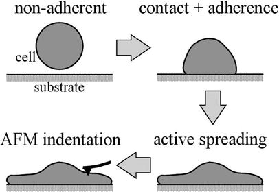
Four configurations for an adherent cell, including an assumed materially isotropic cell in a non-adherent, traction-free reference configuration. Adherence and active spreading likely change the material symmetry from isotropic to anisotropic via an affine deformation-dependent mechanism and possibly active remodeling (not considered explicitly)

Finally, because little is yet known about the specific functional forms of w^k(α^k) for the individual constituents of the cytoskeleton, or the associated values of the material parameters, we nondimensionalize the problem to allow illustrative simulations. Let length, time, and mass scales be, respectively:

28

where d is the diameter of the cell in the non-adherent state (see Fig. 3), ρ is the overall mass density of the cell, and

29

where E is an initial overall elastic modulus of a cell that can be estimated at μ=λ=1, with Γ and Σ obtained from Eq. 10. Consequently, Eq. 4 can be written as:

30

where

31

and x=δ/d.

Illustrative simulations

There is a pressing need for data that are sufficient for identifying specific forms of the constitutive functions (including w^k(α^k) and R^k(ϕ, θ)) and calculating values of the associated material parameters for each constituent. Such data often have to await the development of a theoretical framework, however, for, without a framework, one often does not know what to measure (e.g., overall modulus in a Hertz model versus stiffness and orientation for individual filaments). Notwithstanding the current lack of sufficient data, let us illustrate qualitatively some predictions of the present theoretical framework. Such simulations help us to develop intuition and indeed may help us to interpret future experimental results.

Illustrative mechanical behaviors

Despite scant information on the mechanical behavior of individual filaments (or, more precisely, filament-dominated behaviors that include the effects of select accessory proteins), it appears that these behaviors may be qualitatively similar to those of soft tissue—nonlinear with slight hysteresis (Janmey et al.1991; Liu and Pollack 2002). Hence, one possible form for the 1-D energy function is (Humphrey and Yin 1987):

32

where c^k and c^k₁ are separate material parameters for each family of constituents k. Another possible form is (Lanir 1983):

33

which yields a linear first Piola–Kirchhoff stress vs. stretch relation (note: Eq. 32 reduces to Eq. 33 in the limit as α^k→1, with c^k₂≅c^kc^k₁, no sum on k).

Similarly, despite increasing data from confocal and multi-photon microscopy, there is little information on specific distributions of the orientations of the cytoskeletal filaments. For the purposes of illustration, however, consider a 3-D von Mises–Fisher distribution that results directly from generalizing the von Mises distributions on the 2-D circle (Fisher et al. 1987), namely:

34

This distribution has three parameters: κ, β, and γ. κ is a shape or concentration factor. The larger the value of κ the more the distribution is concentrated towards the direction (β, γ)—see Fig. 4. β and γ are location parameters where the distribution has rotational symmetry about the direction (β, γ). Since R^k is a probability density function, its integral over all possible orientations must satisfy the normalization condition:

35

Fig. 4a, b.

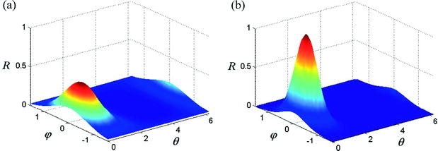
Illustrative (possible) distributions of cytoskeletal filaments given by a von Mises–Fisher distribution function (see Eq. 34). a κ=3, β= 0, γ=π/4. b κ=7, β=0, γ=π/4

Illustrative numerical results

Recalling Fig. 3, let us assume that each family of filaments is randomly distributed in the non-adherent reference configuration. That is, let us assume an initial isotropy despite any stretch-induced anisotropy associated with cell spreading or subsequent stretching of the substrate (note: such stretch-induced changes in orientation can be calculated simply given where M^k and m^k are unit vectors in the direction of a particular filament in original and deformed configurations, respectively). Consequently, let R^k(ϕ, θ)=1/4π. Let the mass fraction of the actin filaments be φ^a=0.038 (Cheng et al. 2000). Material parameters for each filament within the cytoskeleton are chosen such that the actin filaments are stiffer in extension than the microtubules, with the intermediate filaments exhibiting an intermediate extensional stiffness (Janmey et al. 1991). Given such values, we can estimate the mass fractions of the microtubules and intermediate filaments. Assuming that their mass fractions are the same, and using empirical results from Rotsch and Radmacher (2000), which show that the “elastic modulus” of the cell decreases by a factor of three when actin filaments are disrupted, we compare the initial elastic moduli E of two cases, control and actin-disrupted (Eq. 29). Of course, if the filament is disrupted completely, its mass fraction φ^k is zero. The parameters for our calculations are given in Table 1. Finally, for purposes of non-dimensionalization, note that the volume of an average culture cell is approximately 4 pl (Alberts et al. 2002), thus, let d=20 μm. Furthermore, let ρ=1 g/ml for water, which is the most abundant substance in cells (Alberts et al. 2002).

Table 1.

Material parameters for a model cell

Nondimensional parameter	Actin filaments	Microtubules	Intermediate filaments
Mass fraction φ	0.038	0.017	0.017
Stiffness parameter c/E	1.78	1.78	1.78
Material parameter c1	120	50	80
Stiffness parameter c2/E	214	89	142

Note: the volume fraction for actin was taken from Cheng et al. (2000). The volume fractions of the microtubules and intermediate filaments were estimated from Eqs. 10–15 and Eq. 29, and from the experiments of Rotsch and Radmacher (2000). Stiffness and material parameters were assumed based on Janmey (1991); c₂/E was selected for direct comparisons between the exponential and linear models.

Assuming a quasi-static indentation (i.e., D=0 in Eq. 16), consider P–δ (actually Ψ–η) results for different values of the in-plane stretch μ∈[1, 1.12] for both an exponential and a linear behavior (Eq. 32 and Eq. 33) of the filaments and with a flat-ended cylindrical indenter (Fig. 5). Similarly, consider results at a single stretch (μ=1.2) for exponential-type filament behaviors with four different indenter tips (Fig. 6a). If we interpret the slope of the force–depth relation as a measure of the “stiffness” of the cell, we see that both the degree of finite stretch (e.g., degree of spreading) and the geometry of the tip dramatically affect this result, given the same material properties. In particular, only the flat-ended tip yields a linear force–depth relation for the small indentation. The non-flat-tipped indenters contact increasingly more material as they indent deeper. Finally, note that removal of individual constituents reduces the stiffness as expected (Fig. 6b): disruption of the actin filaments can reduce the stiffness substantially, whereas there can be little contribution to the overall cytoskeletal stiffness by the microtubules or intermediate filaments. This observation agrees with the empirical findings of Wakatsuki et al. (2000) and Wu et al. (1998). Although not shown, additional simulations with different values of the material parameters (see Table 1) revealed qualitatively similar results: decreasing the stiffness of the actin dramatically decreased the indentation force at a given indentation depth and tip-geometry, whereas uniformly raising or lowering the values of the parameters had no effect due to the non-dimensionalization.

Fig. 5a, b.

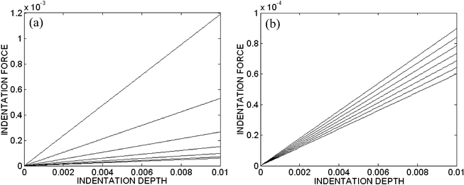
Combined out-of-plane indentation and in-plane equibiaxial stretch for a exponential-type filaments and b linear-type filaments, each indented by a flat-ended circular cylinder with radius 30 nm. Each line corresponds to different in-plane stretches, from lower to upper, of μ=1.00 to 1.12 in steps of 0.02. All results are non-dimensional to emphasize the qualitative responses, not the specific values

Fig. 6a, b.

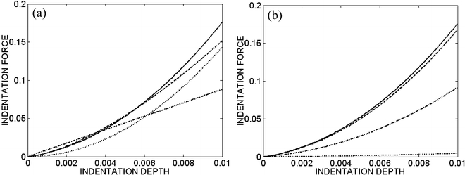
Combined indentation and equibiaxial in-plane stretch, μ=1.2, for the exponential-type filament behavior. a Effects of four different indenter tips: flat-ended circular cylinder with radius a=30 nm (dash-dotted line, which is linear), sphere with radius a=30 nm (dashed line), cone with tip angle 2Φ=75° (dotted line), and blunted cone with tip angle 2Φ=75° and radius a=30 nm (solid line). The nonlinear responses (for all but the flat-ended indenter) are due, in part, to the nonlinearly increasing contact area between the indenter and cell. b Effects of cytoskeleton disrupting drugs with blunted cone, with 2Φ=75° and a=30 nm: control (solid line), actin filament disrupting drugs (dotted line for disruption of all actin filaments, and dash-dotted line disruption of half the actin filaments), and microtubule and intermediate filament disrupting drugs (dashed line). We assume that, if the filament is disrupted completely, the mass fraction φ of the corresponding filament is zero. Note that the predicted behavior is dominated by the actin. All results are non-dimensional to emphasize the qualitative responses, not the specific values

Discussion

Many different experimental methods exist for interrogating the biomechanical properties and mechanobiological responses of cells. They include: atomic force microscopy, magnetic bead cytometry, microfabricated cantilevers, micropatterned surfaces, micropipet aspiration, optical traps, stretching of cells on flexible membranes, laminar flow chambers, and rotating bioreactors. Each method promises new insight into the wonderfully complex structure, function, and properties of living cells, and each warrants rigorous biomechanical analysis. Herein, we focused on atomic force microscopy not only because of its widespread usage, but primarily because of its frequent inappropriate interpretation based on the classical Hertz solution.

Many investigators recognize that the simplifying assumptions inherent to the Hertz solution do not apply in most AFM studies on cells. This was shown convincingly via finite element simulations by Costa and Yin (1999)—they wrote, “Widely applied infinitesimal strain models agreed with FEM results for linear elastic materials, but yielded substantial errors in the estimated properties for nonlinear elastic materials.” Consequently, some employ nonlinear empirical P–δ relations and then try to ascribe meaning to the associated parameters (e.g., Miyazaki and Hayashi 1999; Sato et al. 2000). This approach is limited, however, by the inability to separate structural from material stiffnesses; indeed, it has no biomechanical basis. Alternatively, others appear to rationalize using the Hertz solution by arguing that measuring absolute values of the material properties is less important than delineating relative changes from cell-to-cell or intervention-to-intervention. Finally, some appear to use the Hertz solution simply because of a lack of a viable alternative. Mathur et al. (2001) imply, for example, that there is simply a need for further development of applicable theoretical frameworks. Regardless, there is a pressing need to move beyond the assumptions of a linearly elastic behavior of a single constituent continuum under infinitesimal strains.

The approach and findings of Costa and Yin (1999) represent a pivotal step in improving analyses of AFM experiments. Nonetheless, their finite element solutions are limited, largely because of the use of a commercially available code that is best suited for strain–energy functions that describe the isotropic behavior of single constituent (i.e., materially uniform) continua. Cells, in contrast, contain multiple structurally important constituents that are able to remodel individually to different extents and at different rates. Indeed, recent advances in molecular biology that allow one to selectively modify individual constituents (see, e.g., Wu et al. 1998; Rotsch and Radmacher 2000) necessitate a more general theoretical framework for analysis. Albeit based on a number of simplifying assumptions—e.g., small, quasi-static indentations on equibiaxially stretched cells—the approach presented herein can account for the separate orientations, properties, and deformations of multiple constituents within the cytoskeleton, and, thus, changes in the mechanical response of cells that are induced by biological or mechanical stimuli, such as applying cytoskeleton disrupting drugs or pre-stretch. Indeed, despite the need to introduce particular constitutive relations to numerically illustrate the theory, these can be varied easily as demanded by increasingly better data, thus rendering the overall theory more general.

We emphasize that the two primary uses of such a framework should be to guide experimentation (e.g., highlight what needs to be measured, such as constituent properties, orientations, and mass fractions) and to serve as a check for future finite element analyses of AFM, which will be needed to study additional classes of tests. In particular, the present results cannot be used in cases wherein the indentation is above the nucleus or near the periphery where the effects of the underlying substrate are pronounced. In such cases, finite element analyses will be essential. Likewise, the present results should only be used in tests wherein the indentation is “small” and “quasi-static.” This reminds us again that theory should guide experiment. Finally, the most basic issue is that of the continuum assumption. The dimensions of the cell are on the order of micrometers whereas those of the cytoskeletal filaments are on the order of nanometers, which suggest that a continuum assumption may be reasonable, as used in most papers to date. Nevertheless, the diameter of the indenter is often on the order of 10–50 nm, similar to that of the diameters of the primary constituents, thus, this merits careful attention. This could be addressed, in part, by comparing predictions with additional experiments and would likely be aided by simultaneous imaging of the cytoskeleton. Conversely, one may need to consider larger diameter indenters, particularly ones that are flat-ended, for they alone can yield linear force–depth data. Of course, in the final analysis, as noted by Truesdell and Noll (1965), “Whether the continuum approach is justified, in any particular case, is a matter, not for the philosophy or methodology of science, but for the experimental test.” Each case must be so justified, depending on the particular test and its overall goal. Going beyond a continuum approach will, of course, require remarkably fine detail on the distributions and interactions of all constituents—a significant challenge.

In conclusion, the complex structure and properties of living cells demand continued research into improved models. At the minimum, we should account for the nonlinear material behavior over finite strains of a multi-constituent material. The present paper describes one step toward that goal, one that synthesizes prior work on microstructural models of soft tissues and an analytical solution from finite elasticity. It is hoped that this new model allows improved interpretation of sub-classes of AFM tests and, more importantly, that it provides some direction for further research.

References

- Alberts B, Johnson A, Lewis J, Raff M, Roberts K, Walter P (2002) Molecular biology of the cell. Garland Science, New York
- Beatty MF, Usmani SA (1975) On the indentation of a highly elastic half-space. Q J Mech Appl Math 28:47–62
- Briscoe BJ, Sebastian KS, Adams MJ (1994) The effect of indenter geometry on the elastic response to indentation. J Phys D Appl Phys 27:1156–1162
- Brodland GW, Gordon R (1990) Intermediate filaments may prevent buckling of compressively loaded microtubules. ASME J Biomech Eng 112:319–321 [DOI] [PubMed]
- Cheng Y, Hartemink CA, Hartwig JH, Dewey CF (2000) Three-dimensional reconstruction of the actin cytoskeleton from stereo images. J Biomech 33:105–113 [DOI] [PubMed]
- Costa KD, Yin FCP (1999) Analysis of indentation: implications for measuring mechanical properties with atomic force microscopy. ASME J Biomech Eng 121:462–471 [DOI] [PubMed]
- Fisher NI, Lewis T, Embleton BJJ (1987) Statistical analysis of spherical data. Cambridge University Press, Cambridge
- Fung YC (2002) Celebrating the inauguration of the journal: biomechanics and modeling in mechanobiology. Biomech Model Mechanobiol 1:3–4
- Green AE, Rivlin RS, Shield RT (1952) General theory of small elastic deformations superimposed on finite elastic deformations. Proc R Soc Lond 211A:128–154
- Heidemann SR, Kaech S, Buxbaum RE, Matus A (1999) Direct observations of the mechanical behaviors of cytoskeleton in living fibroblasts. J Cell Biol 145:109–122 [DOI] [PMC free article] [PubMed]
- Herant M, Marganski WA, Dembo M (2003) The mechanics of neutrophils: synthetic modeling of three experiments. Biophys J 84:3389–3413 [DOI] [PMC free article] [PubMed]
- Humphrey JD (2002a) On mechanical modeling of dynamic changes in the structure and properties of adherent cells. Math Mech Sol 7:521–539
- Humphrey JD (2002b) Cardiovascular solid mechanics: cells, tissues, and organs. Springer, Berlin Heidelberg New York
- Humphrey JD, Yin FCP (1987) A new constitutive formulation for characterizing the mechanical behavior of soft tissues. Biophys J 52:563–570 [DOI] [PMC free article] [PubMed]
- Humphrey JD, Halperin HR, Yin FCP (1991) Small indentation superimposed on a finite equibiaxial stretch: implications for cardiac mechanics. ASME J Appl Mech 58:1108–1111
- Janmey PA, Euteneuer U, Traub P, Schliwa M (1991) Viscoelastic properties of vimentin compared with other filamentous biopolymer networks. J Cell Biol 113:155–160 [DOI] [PMC free article] [PubMed]
- Lanir Y (1983) Constitutive equations for fibrous connective tissues. J Biomech 12:423–436 [DOI] [PubMed]
- Liu X, Pollack GH (2002) Mechanics of F-actin characterized with microfabricated cantilevers. Biophys J 83:2705–2715 [DOI] [PMC free article] [PubMed]
- Mathur AB, Collinsworth AM, Reichert WM, Krauss WE, Truskey GA (2001) Endothelial, cardiac muscle and skeletal muscle exhibit different viscous and elastic properties as determined by atomic force microscopy. J Biomech 34:1545–1553 [DOI] [PubMed]
- Miyazaki H, Hayashi K (1999) Atomic force microscopic measurement of the mechanical properties of intact endothelial cells in fresh arteries. Med Biol Eng Comput 37:530–536 [DOI] [PubMed]
- Radmacher M, Tillmann RW, Fritz M, Gaub HE (1992) From molecules to cells: imaging soft samples with the atomic force microscope. Science 257:1900–1904 [DOI] [PubMed]
- Rajagopal KR, Tao L (1995) Mechanics of mixtures. World Scientific, Singapore
- Rotsch C, Radmacher M (2000) Drug-induced changes of cytoskeletal structure and mechanics in fibroblasts: an atomic force microscopy study. Biophys J 78:520–535 [DOI] [PMC free article] [PubMed]
- Sato M, Nagayama K, Kataoka N, Sasaki M, Hane K (2000) Local mechanical properties measured by atomic force microscopy for cultured bovine endothelial cells exposed to shear stress. J Biomech 33:127–135 [DOI] [PubMed]
- Sneddon IN (1965) The relation between load and penetration in the axisymmetric Boussinesq problem for a punch of arbitrary profile. Int J Eng Sci 3:47–57
- Stamenovic D, Ingber D (2002) Models of cytoskeletal mechanics of adherent cells. Biomech Model Mechanobiol 1:95–108 [DOI] [PubMed]
- Treloar LRG (1975) The physics of rubber elasticity. Clarendon Press, Oxford
- Truesdell C, Noll W (1965) The non-linear field theories of mechanics. In: Flugge S (ed) Handbuch der Physik, Vol III/3. Springer, Berlin Heidelberg New York
- Wakatsuki T, Kolodney MS, Zahalak GI, Elson EL (2000) Cell mechanics studied by a reconstituted model tissue. Biophys J 79:2353–2368 [DOI] [PMC free article] [PubMed]
- Wu HW, Kuhn T, Moy VT (1998) Mechanical properties of L929 cells measured by atomic force microscopy: effects of anticytoskeletal drugs and membrane crosslinking. Scanning 20:389–397 [DOI] [PubMed]
- Zhu C, Bao G, Wang N (2000) Cell mechanics: mechanical response, cell adhesion, and molecular deformation. Annu Rev Biomed Eng 2: 189–226 [DOI] [PubMed]