Modeling Surface Growth of Escherichia coli on Agar Plates

Abstract

Surface growth of Escherichia coli cells on a membrane filter placed on a nutrient agar plate under various conditions was studied with a mathematical model. The surface growth of bacterial cells showed a sigmoidal curve with time on a semilogarithmic plot. To describe it, a new logistic model that we presented earlier (H. Fujikawa et al., Food Microbiol. 21:501-509, 2004) was modified. Growth curves at various constant temperatures (10 to 34°C) were successfully described with the modified model (model III). Model III gave better predictions of the rate constant of growth and the lag period than a modified Gompertz model and the Baranyi model. Using the parameter values of model III at the constant temperatures, surface growth at various temperatures was successfully predicted. Surface growth curves at various initial cell numbers were also sigmoidal and converged to the same maximum cell numbers at the stationary phase. Surface growth curves at various nutrient levels were also sigmoidal. The maximum cell number and the rate of growth were lower as the nutrient level decreased. The surface growth curve was the same as that in a liquid, except for the large curvature at the deceleration period. These curves were also well described with model III. The pattern of increase in the ATP content of cells grown on a surface was sigmoidal, similar to that for cell growth. We discovered several characteristics of the surface growth of bacterial cells under various growth conditions and examined the applicability of our model to describe these growth curves.

Generally, microbial growth in liquid is planktonic, whereas the structure of a microbial colony grown on a surface is considerably complex (11, 23). The surfaces of solids, such as would exist on solid foods, are susceptible to attachment by and subsequent growth of microorganisms, where they might exist as a biofilm, a unique microbial community (22). Studies on microbial surface growth, therefore, are thought to be considerably important in many microbiological fields.

Microbial surface growth studies on kinetic parameters such as the rate constant of growth and the lag period have been done by many investigators (8, 18, 21, 27, 32, 33). Some investigators selected the colony size parameters such as the diameter and height as the measures of growth (27, 33). These measures of microbial growth are easy to measure and are for one dimension, but microbial colonies are three-dimensional objects by nature. Other investigators have studied the increase in the cell number of one colony with time (8). However, when we quantitatively evaluate microbial growth on a surface, the total cell numbers of colonies would be more appropriate as the measure of growth than those of a single colony. Thus, some of the investigators measured the increase in the total cell number of microbes inoculated on the surface of a specific food (2, 18, 20, 28). However, few investigators have studied microbial growth curves on a surface (2, 20, 28). Also, the basic characteristics of the population dynamics of microbial cells grown on a surface have not fully been elucidated.

For the last two decades, a number of mathematical models have been developed to quantitatively describe microbial growth in culture media and food (4, 9, 16, 25). Recently, we developed a new logistic model, which is a logistic model extended for the description of microbial growth (12, 13). Our model has the potential to predict bacterial growth at constant and dynamic temperatures in broth and liquid foods. More recently, we slightly modified the model to more precisely describe bacterial growth at the acceleration phase of growth (14, 15).

In the present study, therefore, we studied surface growth patterns of Escherichia coli cells under various conditions and modeled them using our model to evaluate the possibility that the model could describe and predict the surface growth of cells. We have already extensively studied the growth kinetics of this microorganism in liquid culture (12-14).

MATERIALS AND METHODS

Cell preparation.

Cell suspensions of E. coli 1952, which was previously studied for growth in liquid media, were prepared by the method of Fujikawa et al. (12-14). Briefly, bacterial cells were activated on a nutrient agar plate (Nissui Pharmaceuticals, Tokyo, Japan) at 35°C for 24 h. Cells of several well-grown colonies on the plate were incubated in a nutrient broth (Nissui Pharmaceuticals) with shaking at 35 C for 24 h. Cultured cells were washed twice with phosphate buffer (pH 7.0) by centrifugation. Cells were then resuspended in the buffer. This gave a cell suspension of ca. 10⁹ to 10¹⁰ CFU/ml. The cell suspension was then diluted to 1:10⁶ (in most of the experiments) with the nutrient broth and stored at about 5°C before use.

Incubation.

Bacterial cells were surface-grown by using the membrane filter method (3, 19). Portions (1 ml) of the cell suspension prepared above were placed on a sterile filtration membrane with a 0.22-μm pore size and 25 mm in diameter (GSWP02500; Millipore, Bedford, MA) that was already set in a sampling manifold with 12 wells (no. 1225; Millipore). Cells in the suspension were collected on the membrane by vacuum filtration. These procedures were done in a sterile clean bench. The membrane was then placed at the center on the surface of a nutrient agar plate (Nissui Pharmaceuticals) that was already cooled to about 5°C.

Cells on the membranes were incubated in a humidified, programmed incubator (PR-3G; Tabai Espec Co., Osaka, Japan) at a constant or varying temperature (13). Immediately after each incubation period, the membrane in triplicate was taken from the incubator and cooled to about 5°C.

The temperature of the membrane on a plate was monitored with a digital thermometer (AM-7002; Anritsu Meter Co., Tokyo, Japan). The come-up time of the sample to reach a designated temperature was measured for the constant temperature experiment. This period, which was about 24 min for most of the constant temperatures, was taken into consideration (13). For a varying-temperature experiment, sample temperature was measured every 30 s throughout the experiment.

Agar plates with various nutrient levels.

Agar plates with 1/5 and 1/25 nutrient levels of the original nutrient agar plates (15 g of peptone/liter and 5 g of meat extract/liter as nutrients; Nissui Pharmaceuticals) were prepared with agar (Bacto agar; Becton Dickinson, Sparks, MD) and nutrient broth (powder) containing peptone and meat extract (Nissui Pharmaceuticals). Agar plates without any nutrient broth were also prepared. All agar plates contained a constant amount of salt (5 g/liter). Their pHs were not adjusted because they were maintained at about 7 with the buffering action of the agar and the nutrient broth used. In the experiments with the low-nutrient-level agar plates, washed cells were suspended in the phosphate buffer and then collected on a membrane by vacuuming.

Cell counts.

Cells grown on a membrane filter were suspended with 40 ml of buffered peptone water (pH 7.0; Nissui Pharmaceuticals), with Tween 80 in a sterile plastic bag using a stomacher for 1 min. The number of cells in the suspension was counted in duplicate using nutrient agar plates with the surface plating method. After each average (three per datum point) was transformed into the logarithm with base 10, the average and standard deviation of each point were then calculated. The counts of cells on a membrane without incubation were the initial value for each experiment.

ATP measurement.

The ATP content of cells grown on a membrane filter was measured in triplicate by using the firefly luciferin-luciferase method with an ATP analyzer (AF 100; TOA Electronics, Tokyo, Japan). Briefly, cells incubated on the filter membrane were placed with the membrane in a sample well of the analyzer. The ATP content of the cells was then measured with a reagent kit (AF-2L1; TOA Electronics) according to the manufacturer's technical manual. For samples whose ATP contents were over the measurement range of the analyzer, the cells on the membrane filter were suspended in 9 ml of deionized, cool water in a sterile plastic tube by sonicating them for 1 min. The ATP content of the cell suspension was then measured again with the analyzer according to the technical manual. The average of each datum point was then calculated.

Model development.

Recently, we have developed a new logistic model of microbial growth (12, 13). The rate of growth of the model is expressed as follows: dN/dt = rN (1 − N/N_max)(1 − N_min/N)ⁿ (equation 1). Here, N is the population (arithmetic number) of the organism at time t, r is the rate constant of growth, N_max is the maximum population, and N_min corresponds to the inoculum size. n (≥0) is an adjustment factor, which was called c in our previous study (12, 13).

To more precisely describe a linear growth during the acceleration period in a growth curve, we slightly improved equation 1 for the position of the adjustment factor n (14). In the improved model, the factor worked on the fraction N_min/N, instead of the term 1 − N_min/N. The improved model can thus be expressed as follows: dN/dt = rN(1 − N/N_max){1 − (N_min/N)ⁿ} (equation 2). We will denote equations 1 and 2 as models I and II, respectively.

In the present study, we modified model II for the description of the curve of microbial surface growth. As seen later in the results section, surface growth curves were sigmoidal, whereas the curvature during the late exponential phase, or the deceleration phase, was larger than that in liquid medium (13). To represent this, model II was modified in the present study; the Richards model, which is an empirical one, was introduced in the term of 1 − N/N_max of the equation 2. In the Richards model, the term of 1 − N/N_max of the original logistic model is changed to 1 − (N/N_max)^m by introducing a curvature parameter m (>0) (4, 30). The new growth model, therefore, can be described as follows: dN/dt = rN {1 -(N/N_max)^m}{1 -(N_min/N)ⁿ} (equation 3) Here, we will denote equation 3 as model III. Model III can describe sigmoidal curves with various curvatures during the deceleration phase compared to model II. With a larger m, the curvature of the deceleration phase with model III becomes smaller.

Numerical solution of the models.

Equation 3 was solved numerically with the four-order Runge-Kutta method using spreadsheet software (Microsoft Excel), similar to equations 1 and 2 (12-14). Parameter r was set to be a measured rate constant of growth during the exponential phase in an experimental growth curve (12-14). N_max and N_min in the model, which are both the asymptotes, were estimated from experimental data (12-14). Parameters m and n were estimated with the least-squares method that minimizes the means of the square error, MSE, between log-transformed cell concentrations predicted with the model and those observed at the observation points. Namely, parameter n was first estimated by using the experimental data from the initial time to that at the exponential phase, because the parameter strongly affects the duration of the lag period. Parameter m was then estimated by using the whole data set and the estimated n value to evaluate the curvature during the late exponential phase. With those optimal parameter values, growth curves were generated by using model III.

Prediction at a dynamic temperature was done by using the values of parameters in model III studied at the constant temperatures in the same manner as model II (13). Briefly, the value of r at the measured temperature of a time interval during an experimental temperature history was obtained from the Arrhenius model. For parameters m, n, and N_max, the averages at the constant temperatures were used. N_min was determined from a measured initial cell number, N₀.

The Baranyi model for a dynamic temperature was also solved with the four-order Runge-Kutta method for varying-temperature experiments (5). Parameter α₀ in the model was estimated from experiments at constant temperatures, which are shown below. That is, it was obtained from the mean values of the rate constant of growth during the exponential phase, r, and the lag period, lag, at the constant temperatures.

Comparison of growth models.

The parameters of r and lag for curves predicted with model III were estimated (12-14). That is, r was estimated from the slope of the linear portion of the predicted curves using linear regression analysis with Excel. lag was estimated as the period between the initial point and the point where the regression line for the exponential phase intersects the horizontal line penetrating the initial point on the semilogarithmic plot.

Curve fitting to the Baranyi and modified Gompertz models for experimental growth data at constant temperatures was done with software program DMfit, which was kindly provided by J. Baranyi. With the program, we obtained curves fitted to the models by inputting raw data. For parameters mCurv and h₀ in the Baranyi model, the default values (both 10) were used for prediction. Values of r and lag for those Baranyi and modified Gompertz curves were estimated from the generated curves in the same way as those for model III described above.

For r and lag estimated from the growth models, MSE and the correlation coefficients (R²) of linearity between estimated and measured parameter values were evaluated by using Excel.

RESULTS AND DISCUSSION

Growth at constant temperatures.

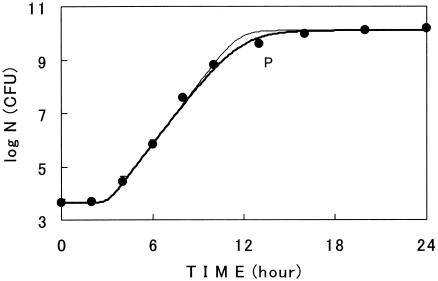
Growth curves of E. coli cells on a membrane surface placed on a nutrient agar plate were sigmoidal at various constant temperatures (10 to 34°C). One of the examples is shown in Fig. 1. The growth curves were successfully described with the new logistic model III. Model III could describe the curvature of the deceleration phase better than model II. That is, in Fig. 1, the difference between the measured and estimated cell numbers using model III with a 13-h incubation (point P) was smaller (0.24 log unit) than that with model II (0.47 log unit). The value of MSE for cell numbers measured and estimated with model III during the growth period (0.021) was also smaller than that with model II (0.034). Similar results for both models were obtained at the other constant temperatures studied (data not shown). These results showed the superiority of model III to model II in the description of growth curves, and therefore model III was used thereafter in the present study.

FIG. 1.

Surface growth curve of E. coli at a constant temperature (30°C). Circles are experimental. Growth curves were described with models II (thin line) and III (thick line). Bars show the standard deviations of the average viable cell counts. The thick line describes model III with m = 0.45. P is a point measured after incubation for 13 h.

Parameter values of model III for the growth curves are listed in Table 1. The values of MSE were very small. The values of m were almost constant at the temperatures studied with the average of 0.58, except for the value at 22°C. The values of n were also almost constant with the average of 3.0 without including the value at 10°C. The values of N_max for the curves were constant (∼10.1 log units).

TABLE 1.

Parameter values of new logistic model III for E. coli surface growth curves on nutrient agar plates at constant temperatures

Parametera	Value at temp (°C):
	10	14	18	22	26	30	34
r (1/h)	0.217	0.266	0.537	0.703	1.05	1.71	2.05
m	0.41	0.66	0.47	1	0.58	0.45	0.48
n	1.3	3.4	2.7	3.9	3.3	2.5	3.6
N0 (CFU)*	103.4	103.6	103.5	103.7	103.8	103.7	103.6
Nmax (CFU)*	109.7	1010.1	1010.1	1010.1	1010.1	1010.1	1010.2
MSE (log unit)	0.037	0.022	0.022	0.0070	0.0042	0.021	0.033

^a*, CFU per membrane.

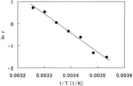
The Arrhenius analysis for r to the temperature was very linear with R² = 0.986 (Fig. 2). The linear regression line in the figure was expressed as follows: ln r = −8,640 × 1/T + 28.9 (equation 4). Here, ln is the natural logarithm, and T is the temperature (K).

FIG. 2.

Arrhenius plot for r to the temperature. Circles are experimental. The straight line is the linear regression line.

The temperature dependency of r was also analyzed with the square-root model, which is widely used (29). The relationship between r and T was expressed as √r = 0.0426 × T − 0.0349. Here, the unit of T is in degrees Celsius (°C). The linearity was very good (R² = 0.977) but slightly lower than that of the Arrhenius plot.

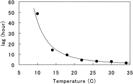
The duration of lag was longer at the lower temperature (Fig. 3). The relationship between lag and T (°C) could be experimentally expressed by using an exponential equation of lag = 15,800 × T^−2.59 with a high R² value of 0.980.

FIG. 3.

Temperature dependency of the duration of lag. Circles are experimental. The line is the regression line with an exponential function.

Model comparison.

Model III was compared to the modified Gompertz and Baranyi models (4, 16), which have been well studied by many investigators, for the growth curves at the constant temperatures. All of the models described the growth curves well (Fig. 4). A curve predicted with one model crossed over the others several times during the growth period. More precisely, model III and the Gompertz model gave slightly better descriptions (less MSE) of the growth curves than the Baranyi model; the average MSE values between predicted and observed cell numbers at temperatures of 10 to 34°C were 0.030, 0.029, and 0.036 (log unit) for model III, the Gompertz model, and the Baranyi model, respectively. There were no significant differences in MSE between two of the three models at a confidence level of 0.95 by the t test. The Gompertz curves were more variable throughout growth (Fig. 4), similar to the growth curves in a liquid (12-14).

FIG. 4.

Comparison of growth prediction by model III to those obtained by the Baranyi and Gompertz models. E. coli growth curve at 26°C was analyzed with the models. Closed circles are experimental. Abbreviations: NLM, new logistic model III (solid line); Bar, Baranyi model (gray line); Gom, Gompertz model (dotted line). Bars show the standard deviations of the average viable cell counts.

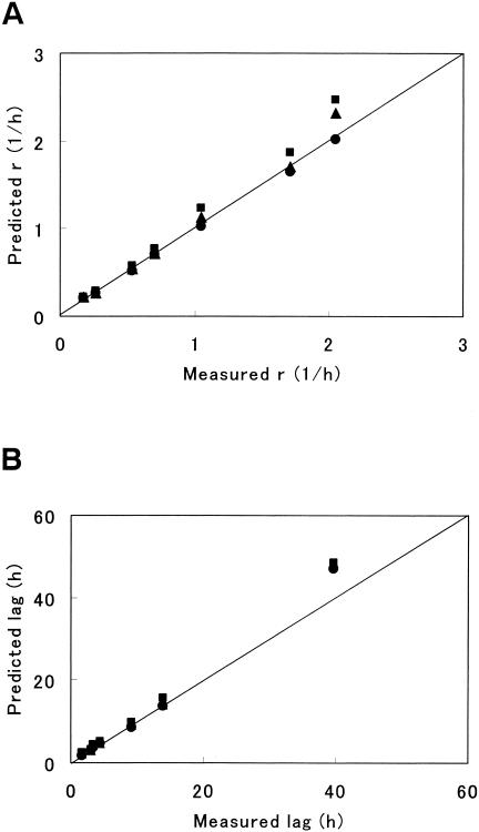
For r and lag, which are the key parameters to characterize a growth curve, model III gave the best estimates among the models (Fig. 5). Model III gave the least MSE and high R² values of linearity for r and lag (Table 2). These results showed that model III was more suitable to describe the surface growth curves than the other models. The Gompertz model had a tendency to overestimate the rate constant (Fig. 5A), similar to growth curves in liquid (13, 26).

FIG. 5.

Comparison of the rate constant (A) and the lag period (B) by model III with those by the Baranyi and Gompertz models. E. coli growth curves at 10 to 34°C were analyzed with the models. Symbols: •, model III; ▴, Baranyi model; ▪, Gompertz model. The straight line is the line of equivalence.

TABLE 2.

Comparison of models for parameters in Fig. 5

Parameter	Indexa	Value obtained with various models
		Model III	Gompertz	Baranyi
r	MSE	0.00090	0.035	0.012
	R2	0.999	0.993	0.991
lag	MSE	7.6	12	11
	R2	0.996	0.998	0.995

^aThe indices were calculated from the predicted and observed values of the parameters.

In the present study, we could not analyze the surface growth curves with the three-phase linear model developed by Buchanan et al. (9) because a curve-fitting program for the model, ABACUS, was unavailable to us. However, from the nature of the model where the rate constant of growth and the lag period are directly incorporated into the model, it could be expected that if our experimental data were analyzed with the model, the estimated values of r and lag would be equal to the measured ones in Fig. 5.

Growth at varying temperatures.

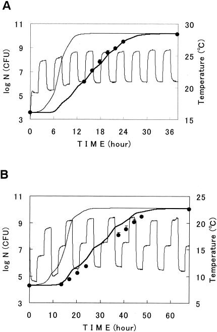
With the parameter values of model III at the constant temperatures studied above, surface growths at varying temperatures were predicted with the model. For r, the Arrhenius equation (i.e., equation 4) was used because of the better linearity than that of the square-root model as described above. For m, n, and N_max, the averages of the observed values that were described above were used, being 0.58, 3.0, and 10^10.1, respectively. As shown in Fig. 6, the model successfully predicted growth with small values of MSE (Fig. 6A, 0.010, and Fig. 6B, 0.14 in log units). These results showed that the kinetics of bacterial surface growth was governed by temperature and that the model had the potential to predict the growth curves at various temperature profiles. There was a tendency that predictions at lower temperature ranges were slightly greater than actual measured cell counts (Fig. 6B), but the reason for this was not understood.

FIG. 6.

Growth curves of E. coli at dynamic temperatures (A and B). Circles are experimental. Thick and thin lines describe curves predicted with model III and the Baranyi model, respectively. Periodic thin lines describe the surface temperatures of the samples. Bars show the standard deviations of the average viable cell counts.

Predictions at various temperatures were also done with the square-root model for r in a preliminary study. As a result, predictions with the Arrhenius model were slightly better than those with the root square model (data not shown).

Predictions with the Baranyi model were studied at various temperatures in comparison with model III. Several investigators applied the Baranyi model to microbial growth at various temperatures (1, 6, 7, 20). The model was found to considerably overestimate bacterial growth in our study (Fig. 6A and B). This overestimation had already taken place during the first half of the observation period. Here, parameter α₀ was experimentally estimated to be 0.0187. The overestimation with the Baranyi model was also observed by other investigators (1, 6, 7, 20). They also reported that growth curves described with the model strongly change with the value of α₀ (1, 6, 7, 20). The same phenomena were observed in the present study. There were great differences in curve fittings with the model between constant and varying temperatures in our study. Baranyi and Roberts (4) reported that the value of the parameter is related to the physiological state of inoculated cells, but we cannot know in advance the optimal value of the parameter that gives the best prediction, especially at a varying temperature.

Growth at various initial cell numbers and nutrient levels.

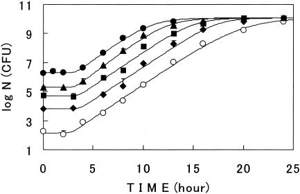
When E. coli cells grew on a surface at various initial cell numbers, the growth curves were also sigmoidal and well described with model III (Fig. 7). Regardless of the variety of the initial cell numbers, the rate constant of growth was constant, and the maximum cell population converged at a given value (Table 3). This was also observed with E. coli growth in a liquid at the optimal and suboptimal temperatures (10, 13), but similar studies on surface growth have not been carried out to our knowledge. The values of m and n for the curves in Fig. 7 were also independent of the initial cell load (Table 3).

FIG. 7.

Surface growth curves of E. coli at various initial numbers of cells. Cells were grown at 26°C. Symbols are the averages of the samples. Lines describe model III. Bars show the standard deviations of the average viable cell counts.

TABLE 3.

Parameter values of model III for surface growth curves at various initial cell numbers in Fig. 7

Parameter	Value obtained with an initial cell number (CFU)a of:
	102.2	103.8	104.7	105.3	106.3
r (1/h)	1.1	1.0	1.1	1.2	1.1
m	0.40	0.73	0.66	0.54	0.60
n	4.1	3.3	3.3	3.3	3.4
Nmax (CFU)a	1010.1	1010.1	1010.1	1010.1	1010.1
MSE (log unit)	0.020	0.036	0.038	0.010	0.0043

^aCFU per membrane.

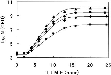
The nutrient level of a solid surface where microorganisms attach differs with place. Surface growth curves at various nutrient levels were then studied. The growth curves were sigmoidal and well described with model III (Fig. 8). Parameter values analyzed with the model are listed in Table 4. With the lower nutrient level agar plates, the rate of growth became slower and the value of N_max was lower. On the other hand, the duration of lag was almost constant.

FIG. 8.

Surface growth curves of E. coli at various initial nutrition levels. Cells were grown at 30°C. Symbols: ▴, nutrient agar (the control); •, 1/5 nutrient level agar; ⧫, 1/25 nutrient level agar; ▪, agar without nutrients added. Lines describe model III. Bars show the standard deviations of the average viable cell counts.

TABLE 4.

Parameter values of model III for surface growth curves at various nutrient levels in Fig. 8

Parameter	Value obtained at nutrient level:
	1	1/5	1/25	0
r (1/h)	1.7	1.5	1.5	0.98
lag (h)	3.0	2.9	3.0	3.4
m	0.45	0.49	0.44	0.55
n	2.5	3.0	2.9	3.8
Nmax (CFU)a	1010.1	109.45	108.9	107.75
MSE (log unit)	0.021	0.010	0.019	0.0047

^aCFU per membrane.

On agar plates without any (organic) nutrients added, bacterial cells did grow to a certain level (Fig. 8). This meant that the agar itself (Bacto agar) had a certain amount of nutrients to allow bacterial growth.

Comparison with growth in a liquid.

The surrounding environment on a surface for microorganisms was considered to be very different from that in a liquid. Also, the freedom of microbial growth on the surface would be strictly limited compared to that in a liquid. Growth curves on a surface were thus compared to that in a liquid. Here, the experiments in a liquid (nutrient broth) were carried out by using methods we reported previously (13).

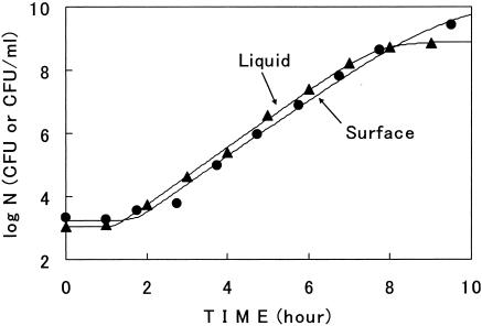
The growth curves on a surface at constant temperatures were very similar to those in a liquid. One example is shown in Fig. 9. In this figure, the values of r and lag of the growth curve on the surface (2.05 1/h and 1.65 h) were very similar to those in the liquid (2.09 1/h and 1.24 h). The maximum cell numbers at the stationary phase were 10^10.2 (CFU per membrane) on the surface and 10^8.9 (CFU/ml) in the liquid in Fig. 9. The Arrhenius plot for r in the liquid at constant temperatures was also similar to that on the surface (data not shown). The only kinetic difference between them was the curvature in the deceleration phase of the growth curve, as observed in Fig. 1. In Fig. 9, m = 0.48 in model III for the surface, whereas m = 1 for the liquid (equal to model II).

FIG. 9.

Comparison of the growth curve on a surface with that in a liquid. Cells were grown at 34°C. Symbols: •, surface; ▴, liquid. Lines describe model III. Cells in the liquid were grown in nutrient broth without shaking.

It is interesting that while nutrients come to the bacterial cells from one vertical direction (for the agar plate) on a surface and from every direction in a liquid, the growth curve on the surface was almost the same as that in the liquid. Generally, the diffusion rate and the amount of nutrients are the limiting factors on microbial growth (9), as seen in Fig. 8. However, this might not be the case here, because the media for both growth analyses, which were broth and nutrient agar plate, contained a lot of nutrients for microbial growth.

Comparison with increase in ATP.

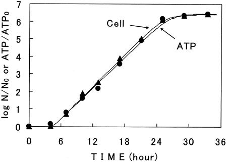
Growth in cell number on a surface was compared to the increase in the ATP content of cells grown under the same conditions at constant temperatures. The increases in the ATP contents of cells during the incubation showed sigmoidal curves, similar to the growth curves as shown in Fig. 1. One example is shown in Fig. 10. The ATP curves were also successfully described with model III (Fig. 10). The ATP curves were coincident with the growth curves at the temperatures studied; the values of r and lag in the two curves in this figure were 0.70 1/h and 4.5 h for cell growth and 0.67 1/h and 4.7 h for the ATP increase, respectively. At some of the temperatures studied, the rate of ATP increase slightly preceded the cell growth; the ATP curve had a slightly shorter lag period. These results showed that the kinetics of the increase in the ATP content of cells was generally similar to that of the cell population.

FIG. 10.

Comparison of the ATP increase curve with the growth curve at 22°C. Symbols: •, ATP content; ▴, cell number. The vertical axis is the logarithm of the ratio of cell number (N) or ATP content (ATP) to the initial value (N₀ or ATP₀). Lines describe model III.

These results led to the speculation that the ATP content of cells on a surface could be a measure of cell growth. The ATP measurement for microbial cells with the firefly luciferin-luciferase method is rapid and simple (17, 31). It takes less than 1 min to measure a sample with the ATP analyzer that we used. Thus, it can be a useful tool for the evaluation of microbial growth on a surface. The relationship between the cell number and ATP content for surface growth at various temperature patterns needs to be studied.

In the present study, we analyzed the surface growth kinetics of bacterial cells with the membrane filter method (3, 19). Here, the substances needed for microbial growth such as nutrients and water passed through the membrane from the agar plate to cells. Some investigators inoculated bacterial cells directly on the surface of an agar plate (2, 21, 24). The membrane filter method has several technical advantages. First, the method is convenient with cells. That is, we can easily transfer cells grown on a membrane to another place. For viable cell counting, these investigators (2, 21, 24) stomached agar with grown cells in a plastic bag. However, agar fractions generated by stomaching might contaminate the cell suspension which is used for viable cell counting. In the present study, stomaching did not fraction the membrane. Second, another measurement for growth on a membrane, such as the ATP content shown in the present study, can be done. Third, the experimental conditions such as cell density in a given surface area on the membrane, is easily controlled, as shown in Fig. 7.

The new logistic models II and III that we have proposed thus far are models extended from the original logistic model in structure. From our previous and present studies (12-15), we think that we can present a generic form of our models for the description of microbial growth curves. That would be model III. That is, when m = 1, it is equal to model II, as shown in Fig. 9. A sigmoidal curve described with model III changes with the values of m and n. Namely, parameter m is related to the curvature during the deceleration period and n is related to lag; with a smaller n, the model describes a growth curve with a longer lag period, and vice versa (13, 14).

Our studies showed that regardless of the complexity of the microbial colony structure on a surface (11, 23), the growth kinetics of a cell population is simple under the experimental conditions in the present study. That is, the surface growth curves were sigmoidal and could be described and predicted with a simple mathematical model such as model III. We are currently studying growth curves of the E. coli strain inside a solid food. Interestingly, growth curves inside the solid, which contains a considerably small volume of air, were very similar to growth curves in a liquid and on a surface at constant temperatures. Also, the growth curves inside the solid were well described with model III. We would like to further study microbial growth patterns inside a solid. We think that a systematic understanding is needed for microbial population dynamics in various fields where microorganisms grow.

REFERENCES

- 1.Alavi, S. H., V. M. Puri, S. J. Knabel, R. H. Mohtar, and R. C. Whiting. 1999. Developing and validation of a dynamic growth model for Listeria monocytogenes in fluid whole milk. J. Food Prot. 62:170-176. [DOI] [PubMed] [Google Scholar]
- 2.Amanatidou, A., E. J. Smid, and L. G. M. Gorris. 1999. Effect of elevated oxygen and carbon dioxide on the surface growth of vegetable-associated micro-organisms. J. Appl. Microbiol. 86:429-438. [DOI] [PubMed] [Google Scholar]
- 3.American Public Health Association. 1992. Membrane filter method (9215 D). In Standard methods for the examination of water and wastewater, 18th ed. American Public Health Association, Washington, D.C.
- 4.Baranyi, J., and T. A. Roberts. 1994. A dynamic approach to predicting bacterial growth in food. Int. J. Food Microbiol. 23:277-294. [DOI] [PubMed] [Google Scholar]
- 5.Baranyi, J., and T. A. Roberts. 1995. Mathematics of predictive food microbiology. Int. J. Food Microbiol. 26:199-218. [DOI] [PubMed] [Google Scholar]
- 6.Baranyi, J., T. P. Robinson, A. Kaloti, and B. M. Mackey. 1995. Predicting growth of Brochothrix thermosphacta at changing temperature. Int. J. Food Microbiol. 27:61-75. [DOI] [PubMed] [Google Scholar]
- 7.Bovill, R., J. Bew, N. Cook, M. D'Agostino, N. Wilkinson, and J. Baranyi. 2000. Predictions of growth for Listeria monocytogenes and Salmonella during fluctuating temperature. Int. J. Food Microbiol. 59:157-165. [DOI] [PubMed] [Google Scholar]
- 8.Brocklehurst, T. F., G. A. Mitchell, and A. C. Smith. 1997. A model experimental gel surface for the growth of bacteria on foods. Food Microbiol. 14:303-311. [Google Scholar]
- 9.Buchanan, R. L., R. C. Whiting, and W. C. Damert. 1997. When is simple good enough: a comparison of the Gompertz, Baranyi, and three-phase linear models for fitting bacterial growth curves. Food Microbiol. 14:313-326. [Google Scholar]
- 10.Coleman, M. E., M. L. Tamplin, J. G. Phillips, and B. S. Marmer. 2003. Influence of agitation, inoculum density, pH, and strain on the growth parameters of O157:H7: relevance to risk assessment. Int. J. Food Microbiol. 83:147-160. [DOI] [PubMed] [Google Scholar]
- 11.Fujikawa, H. 1994. Diversity of the growth patterns of Bacillus subtilis colonies on agar plates. FEMS Microbiol. Ecol. 13:159-168. [Google Scholar]
- 12.Fujikawa, H., A. Kai, and S. Morozumi. 2003. A new logistic model for bacterial growth. J. Food Hyg. Soc. Japan 44:155-160. [DOI] [PubMed] [Google Scholar]
- 13.Fujikawa, H., A. Kai, and S. Morozumi. 2004. A new logistic model for Escherichia coli at constant and dynamic temperatures. Food Microbiol. 21:501-509. [Google Scholar]
- 14.Fujikawa, H., A. Kai, and S. Morozumi. 2004. Improvement of new logistic model for bacterial growth. J. Food Hyg. Soc. Japan 45:250-254. [DOI] [PubMed] [Google Scholar]
- 15.Fujikawa, H., and S. Morozumi. Modeling Staphylococcus aureus growth and enterotoxin production in milk. Food Microbiol., in press. [DOI] [PubMed]
- 16.Gibson, A. M., N. Bratchell, and T. A. Roberts. 1987. The effect of sodium chloride and temperature on the rate and extent of growth of Clostridium botulinum type A in pasteurized pork slurry. J. Appl. Bacteriol. 62:479-490. [DOI] [PubMed] [Google Scholar]
- 17.Goldschmidt, M. C., and D. Y. C. Fung. 1979. Automated instrumentation for microbiological analysis. Food Technol. 3:63-70. [Google Scholar]
- 18.Ingham, S. C., J. A. Losinski, B. K. Dropp, L. L.Vivio, and D. R. Buege. 2004. Evaluation of Staphylococcus aureus growth potential in ham during a slow-cooking process: use of predictions derived from the U.S. Department of Agriculture Pathogen Program Modeling Program 6.1 Predictive Model and an inoculation study. J. Food Prot. 67:1512-1516. [DOI] [PubMed] [Google Scholar]
- 19.Jay, J. M. 1992. Modern food microbiology, 4th ed., p. 101. Chapman and Hall, New York, N.Y.
- 20.Koseki, S., and S. Isobe. 2005. Prediction of pathogen growth on iceberg lettuce under real temperature history during distribution from farm to table. Int. J. Food Microbiol. 104:239-248. [DOI] [PubMed]
- 21.Koutsoumanis, K. P., P. A. Kendall, and J. N. Sofos. 2004. A comparative study on growth limits of Listeria monocytogenes as affected by temperature, pH and aw when grown in suspension or on a solid surface. Food Microbiol. 21:415-422. [Google Scholar]
- 22.Madigan, M. T., J. M. Martinko, and J. Parker. 2000. Block biology of microorganisms, 9th ed., p. 646. Prentice Hall, Upper Saddle River, N.J.
- 23.Mattilla, T., and A. J. Frost. 1988. Colonization of beef and chicken muscle surfaces by Escherichia coli. Food Microbiol. 5:219-230. [Google Scholar]
- 24.McKay, A. L., and A. C. Peters. 1995. The effect of sodium chloride concentration and pH on the growth of Salmonella typhimurium colonies on solid medium. J. Appl. Microbiol. 79:353-359. [DOI] [PubMed] [Google Scholar]
- 25.McMeekin, T. A., J. N. Olley, T. Ross, and D. A. Ratkowsky. 1993. Predictive microbiology: theory and application. Research Studies Press, Taunton, United Kingdom.
- 26.Membre, J.-M., T. Ross, and T. McMeekin. 1999. Behavior of Listeria monocytogenes under combined chilling processes. Lett. Appl. Microbiol. 28:216-220. [DOI] [PubMed] [Google Scholar]
- 27.Membre, J.-M., K. Martine, and C. Chene. 2001. Growth rate and growth-no-growth interface of Penicillium brevicompactum as functions of pH and preservative acids. Food Microbiol. 18:531-538. [Google Scholar]
- 28.Oscar, T. P. 1999. Response surface models for effects of temperature and previous growth sodium chloride on growth kinetics of Salmonella Typhimurium on cooked chicken breast. J. Food Prot. 12:1470-1474. [DOI] [PubMed] [Google Scholar]
- 29.Ratkowsky, D. A., R. K. Lowry, T. A. McMeekin, A. N. Stokes, and R. E. Chandler. 1983. Model for bacterial culture growth rate throughout the entire biokinetic temperature range. J. Bacteriol. 154:1222-1226. [DOI] [PMC free article] [PubMed] [Google Scholar]
- 30.Tsoularis, A., and J. Wallace. 2002. Analysis of logistic growth models. Math. Biosci. 179:21-55. [DOI] [PubMed] [Google Scholar]
- 31.Vanne, L., M. Karwoski, S. Karppinen, and A.-M. Sjoberg. 1996. HACCP-based food quality control and rapid detection methods for microorganisms. Food Cont. 7:263-276. [Google Scholar]
- 32.Wilson, P. D. G., T. F. Brocklehurst, S. Arino, D. Thuault, M. Jakobsen, M. Lange, J. Farkas, J. W. T. Wimpenny, and J. F. Van Impe. 2002. Modelling microbial growth in structured foods: toward a unified approach. Int. J. Food Microbiol. 73:275-289. [DOI] [PubMed] [Google Scholar]
- 33.Winpenny, J. W. T. 1979. The growth and form of bacterial colonies. J. Gen. Microbiol. 114:483-486. [DOI] [PubMed] [Google Scholar]