Neurons of the cerebral cortex exhibit precise interspike timing in correspondence to behavior

Abstract

We show that times of spikes can be very precise. In the cerebral cortex, where each nerve cell is affected by thousands of others, it is the common belief that the exact time of a spike is random up to an averaged firing rate over tens of milliseconds. In a brain slice, precise time relations of several neurons have been observed. It remained unclear whether this phenomenon can also be observed in brains of behaving animals. Here we show, in behaving monkeys, that time intervals between spikes, measured in correspondence to a specific behavior, may be controlled to within the milliseconds range.

As known, most nerve cells in the brain communicate with each other by standard pulses called action potentials (or spikes). In the cerebral cortex, where each nerve cell is affected by thousands of others (1, 2), the common belief, so far, is that each neuron represents one aspect of the mental processes not by precise firing time, but by elevating its firing rate (3). However, if time relations among different neurons could be precisely controlled and read out, complex representations could be built from simpler ones efficiently and very fast (4-6). In a brain slice, precise time relations among several neurons have been observed (7). Could this phenomenon be also observed in brains of behaving animals? Here, we use data-mining techniques and rigorous statistic testing to test the precision of time intervals between spikes of different neurons. We show, in behaving monkeys, that when time intervals between spikes of different neurons are measured in correspondence to a specific behavior, timing may be controlled to the milliseconds range with the best case reaching 0.5 ms.

Experiments Description and Drawings Analysis

In our experiments, single unit activity was recorded from eight microelectrodes inserted into the motor and premotor cortices of a monkey while it was freely scribbling. Spike data analysis was carried for two sets of measurements. In the first set (consisting of 3 experimental days), time resolution of recording was 1 ms, whereas in the second set (consisting of 5 other days), it was 0.1 ms.

Repeated scribbling paths were extracted by data-mining algorithms (8, 9). These paths are called drawing components. In a typical day there are 12-25 such drawing components. Fig. 1 illustrates the monkey's drawings and two simple drawing components.

Fig. 1.

Examples for two drawing components. Thirty seconds of drawing is shown in each box. The hand position was sampled 100 times per s (dots in the drawing). The monkey mostly drew in a counter-clockwise direction (axes are in millimeters). (a) Occurrences of the drawing component: “transitions of drawing direction from a range of 180-210° to a range of 210-240°” are marked by thicker dots. (b) Occurrences of the drawing component: “transitions of drawing velocity from a range of 20-30 cm/s to a range of 10-20 cm/sec” are marked by thicker dots.

The Main Idea

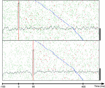
To determine whether there are any precise timing relations between the spikes of two neurons and the drawing, we selected a time slice before the start of each drawing component. For a given pair of neurons, we counted how many times a spike in the first neuron was followed by a spike in the second neuron within each of 50 particular time intervals. For the first set of measurements, these intervals were 0-1 ms, 2-3 ms,..., 98-99 ms, and for the second set they were 0-0.9 ms, 1-1.9 ms, 2-2.9 ms,..., 49-49.9 ms. The interval that repeated the largest number of times was hypothesized to show precise firing times in relation to this particular drawing component. For example, the interval 90-91 ms between neuron 1 from electrode 8 (denoted by 8.1) and neuron 2 from electrode 1 (denoted by 1.2) repeated 372 times within the time window 400 ms to 100 ms before the drawing component that was illustrated in Fig. 1b. Sixty-two of these repetitions are depicted in Fig. 2 (uniformly distributed such that 1 of each 6 is shown). The drawing component itself occurred 1,324 times in the data, so that 25% of its occurrences were preceded by that neural component. Fig. 2 shows one of the relations between a certain drawing component and a certain pair of neurons in this recording day.

Fig. 2.

Dot display showing occurrences of a frequent interspike interval around occurrences of the drawing component that was shown in Fig. 1b. (Upper) Firing times of unit 8.1. (Lower) Firing times of unit 1.2. Each linelet represents a single spike. Each of the 62 lines in both panels shows that spikes occurred around the appropriate 62 (chosen out of 372) occurrences of the drawing component, in which it was preceded at least once by the interval 90-91 ms in the window of 0.4-0.1 s before the start of the drawing component. Linelets representing spikes that took part in the selected interval are colored red. The rasters were aligned on the first spike of the selected interval. If the same interval appeared twice around the same movement, the first occurrence was used for alignment, and the other occurrences appear as red linelets somewhere else along the raster. The time of onset of the drawing is colored blue. Trials are sorted by increasing delays between the neural intervals and the drawing components. The gray line in each panel represents the average firing rate considering all 372 common occurrences using bins of 9 ms. (Scale bars: 50 spikes per s.)

Are these 372 occurrences random? To assess the probability of chance events we generated 1,000 surrogate spike trains by randomly teetering the time of each spike within 10 ms around its real time. For each of these surrogates, we used the same idea for counting all possible intervals between neurons 8.1 and 1.2, which were repeated around the same drawing component during the same time slice. Similarly, the maximal frequency of these intervals was taken as a representative of that surrogate. In the example shown in Fig. 2, these 1,000 maximal frequencies tended to be significantly smaller than 372. Their mean and their variance were used to estimate the probability of these 372 repetitions, assuming normal distribution of counts. For this drawing component and pair of neurons, the mean was 350.678 and the standard deviation was 5.01, yielding a probability of 0.00001.

Is this truly so unlikely? Probably not. The counting process is most probably not distributed normally, so that assessing probability by the mean and variance may be misleading. A much more complicated issue involves finding a rare event for all 12 drawing components recorded that day. We analyzed all of the 50 possible pairs of neurons on that day, all 50 possible time intervals for each pair, and for 7 different time slices around the start of each of the drawing components. Picking the rarest event out of all these possibilities should yield a highly unlikely event. Hence, we need to assess the likelihood of finding such low probabilities when multiple trials are conducted.

Statistical Analysis

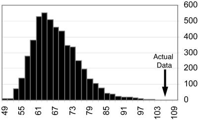
A solution that can be used to test the null hypothesis that spike times are random within a window of width W was offered.¶ If this null hypothesis is true, then replacing the time of each spike by a randomly selected time within W around its true time should not affect any of the statistics extracted from the spike times. To use this idea, we need to describe the entire set of relations between firing intervals and drawing by one statistic. To do so, we defined a statistic based on the 10 least likely relations between pairs of spikes and any of the drawing components. We termed this the relations score. Intuitively, the relations score gets larger as the existing relations are less likely to exist by chance (see The Computation of Relations Score in the supporting information, which is published on the PNAS web site). For each recording day, we computed a relations score for the actual data. Then, we randomly teetered all spike times within some time window W and recomputed it for the teetered data. Independent teetering was done 5,000 times (for the first set of measurements) or 1,000 times (for the second set), and a histogram of the relation scores for teetered data were constructed. After each teetering, all of the parameters for extracting the relations score were reevaluated to get the highest possible value for each teetered data. Fig. 3 illustrates this histogram for W = 10 ms. As stated above, all computations of relations score for each teetered data were done de novo by the same process as was done for the actual data (including multiple trials of all possible drawing components, pairs of neurons, time intervals, and time slices).

Fig. 3.

Distribution of relations scores for surrogate spike trains and the actual data. Five thousand surrogate spike trains were independently generated by teetering spike times within 10 ms. For each of these, a relations score was extracted. The distribution of these relations-score values was estimated by a histogram. The actual data had a value of 106.37 (arrow). None of the 5,000 surrogate trains had a value above it. Hence, the p value for the actual data were estimated as <1/5,000.

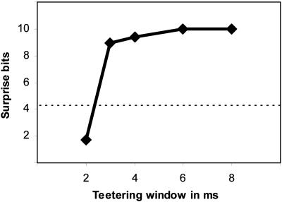
This method was used to estimate the probability, p, of the relations-score value of the actual data. From this p, we derived the surprise value, which was defined as the value of -log₂(p). Fig. 4 shows the surprise values for one recording session, obtained when spike times were teetered within different windows between 2 ms and 8 ms. Clearly, teetering within 3 ms already had a significant effect on the surprise value. Thus, Fig. 4 already indicates that the spike times of the cortical neurons are accurate within 3 ms. Although we used 2-ms bins for measuring the intervals in that day, note that teetering by 2 ms is not pointless, because of the fact that intervals are binned only after teetering is done. Because the original data are measured at a resolution of 1 ms in this case, intervals still may be damaged by teetering.

Fig. 4.

Surprise values for different teetering windows. The abscissa is the teetering window, and the ordinate is the surprise value. The horizontal line shows the surprise value for significance of 0.05. Thus, teetering within 3 ms already had a significant effect.

Significant relations-score values were observed in 3 days (out of 3) for the first set of measurements and in 3 (out of 5) for the second set in this study (total of 6 significant days). For the 3 days of the first set, the smallest teetering windows producing significant results were 3 ms (shown here), 6 ms, and 12 ms. For the 3 days of the second set, these windows were 0.5 ms, 3 ms, and 4 ms. Note that this represents an upper bound for the resolution. One may find that a different statistic can indicate even higher time precision.

When the same procedure was repeated step by step for the neural data around randomly selected points in time (instead of time occurrences of drawing components), no significant surprise values were found (for a teetering window W of 10 ms). Thus, we only obtained significant time relations by relating the neural intervals to specific features in the behavior. Furthermore, no significant surprise values were found when the same procedure was repeated taking a teetered neural data instead of the original data.

Discussion

Numerous studies have reported precise time relations among spikes in the cortex (10-16). In some cases it was claimed that the results were attributed to insufficient statistics (17, 18). In some cases the analysis was limited to precise synchrony, and in some cases no relations to behavior were possible.

Our null hypothesis that spike times are not determined within W ms can be easily tested by teetering. We were able to show that in the most extreme case the null hypothesis could be rejected for W = 0.5 ms. However, there are cellular mechanisms and experimental artifacts that may generate precise spike timing. These include the following: (i) neurons can recover rapidly from the refractory period; (ii) spike intervals within a burst may repeat with high precision; (iii) periodic activity driven by internal pace-maker processes (not due to network oscillations); (iv) dead time for spike detection when recording is made through the same electrode; (v) sharp on or off responses to an external stimulus with abrupt onset (or offset). By considering only intervals between spikes of units recorded with different electrodes, we avoided precise intervals that could be ascribed to i, ii, iii, or iv above. The continuous drawing motion does not generate abrupt time markers that might be responsible for v. Examinations of dot displays as given in Fig. 2 show that the involved spikes (red linelets) were isolated, not periodic, and not located at the onset of sharp changes in activity rates.

Fig. 2 provides further indications that the relations between the neural interval and the drawing component were not random or due to trivial artifacts. First, in both panels the firing rate is stationary. In this condition, had the red marks been random, the spike density around these dots marks should have approximated the autocorrelation function that must be symmetric. However, the little troughs on both sides of the peak (relative refractoriness) are not symmetric. The difference is significant at 0.0002. Second, in dot displays showing another unlikely relations, the delays between the neuronal component and the drawing component (blue marks) were not evenly distributed between -0.4 and -0.1 s, as might be expected for chance relations (see the supporting information).

One would hope to see one-to-one relations between precise firing intervals and drawing components. This is not found here, probably because of the sparse sampling. We record from a score of neurons from a region containing hundreds of thousands. However, the relation of our findings to behavior is underscored by the fact that when random time points (rather than start of drawing components) were chosen, no significant relations scores were found.

These findings, highlighting the precision of spike times in the cortex, raise three types of questions concerning their generation, the way they are read out, and their use. Previous research has shown that synfire chains may produce and read out such precise timing (19), and this property may be used for the dynamic binding of components into a whole (6). Whether the nervous system takes advantage of these features remains open to debate.

References

- 1.Abeles, M. (1991) Corticonics: Neural Circuits of the Cerebral Cortex (Cambridge Univ. Press, New York).
- 2.Braitenberg, V. & Shuez, A. (1998) Cortex: Statistics and Geometry of Neuronal Connectivity (Springer, Berlin).
- 3.Barlow, H. B. (1972) Perception 1, 371-394. [DOI] [PubMed] [Google Scholar]
- 4.Malsburg, C. (1981) MPI Biophysical Chemistry, Internal Report 81-82; reprinted in Malsburg, C. (1994) Models of Neural Networks II, eds. Domany, E., van Hemmen, J. L. & Shulten, K. (Springer, Berlin), pp. 95-119.
- 5.Bienenstock, E. (1996) in Brain Theory: Biological Basis and Computational Properties, eds. Aertsen, A. & Braitenberg, V. (Elsvier, Amsterdam), pp. 269-300.
- 6.Shastri, L. & Ajjanagadde, V. (1993) Behav. Brain Sci. 16, 417-494. [Google Scholar]
- 7.Ikegaya, Y., Aaron, G., Cossart, R., Aronov, D., Lampl, I., Ferster, D. & Yuste, R. (2004) Science 23, 559-564. [DOI] [PubMed] [Google Scholar]
- 8.Mannila, H., Toivonen, H. & Verkamo, A. I. (1995) in Proceedings of the First International Conference on Knowledge Discovery and Data Mining, eds. Fayyad, U. M. & Uthurusamy, R. (AAAI Press, Menlo Park, CA), pp. 210-215
- 9.Mannila, H. & Toivonen, H. (1996) in Proceedings of the Second International Conference on Knowledge Discovery and Data Mining, eds. Simoudis, E., Han, J. & Fayyad, U. (AAAI Press, Menlo Park, CA), pp. 146-151.
- 10.Hastopoulos, N., Geman, S., Amarasingham, A. & Bienenstock, E. (2003) Neurocomputing 52-54, 25-29. [Google Scholar]
- 11.Gray, C. M. & Singer, W. (1989) Proc. Natl. Acad. Sci. USA 86, 1698-1702. [DOI] [PMC free article] [PubMed] [Google Scholar]
- 12.Singer, W. & Gray, C. M. (1995) Annu. Rev. Neurosci. 18, 555-586. [DOI] [PubMed] [Google Scholar]
- 13.Riehle, A., Grun, S., Diesmann, M. & Aertsen, A. (1997) Science 278, 1950-1953. [DOI] [PubMed] [Google Scholar]
- 14.Abeles, M. & Gat, I. (2001) J. Neurosci. Methods 107, 141-154. [DOI] [PubMed] [Google Scholar]
- 15.Nadasdy, Z., Hirase, H., Czurko, A., Csicsvari, J. & Buzsaki, G. (1999) J. Neurosci. 19, 9497-9507. [DOI] [PMC free article] [PubMed] [Google Scholar]
- 16.Villa, A. E., Tetko, I. V., Hyland, B. & Najem, A. (1999) Proc. Natl. Acad. Sci. USA 96, 1106-1111. [DOI] [PMC free article] [PubMed] [Google Scholar]
- 17.Oram, M. W., Wiener, M. C., Lestienne, R. & Richmond, B. J. (1999) J. Neurophysiol. 81, 3021-3033. [DOI] [PubMed] [Google Scholar]
- 18.Baker, S. & Lemon, R. N. (2000) J. Neurophysiol. 84, 1770-1780. [DOI] [PubMed] [Google Scholar]
- 19.Abeles, M., Vaadia, E., Bergman, H., Prut, Y., Haalman, I. & Slovin, H. (1993) Concepts Neurosci. 4, 131-158. [Google Scholar]
Associated Data
This section collects any data citations, data availability statements, or supplementary materials included in this article.