Abstract
We visualized synchronous dynamic brain networks by using prewhitened (stationary) magnetoencephalography signals. Data were acquired from 248 axial gradiometers while 10 subjects fixated on a spot of light for 45 s. After fitting an autoregressive integrative moving average model and taking the residuals, all pairwise, zero-lag, partial cross-correlations ( ) between the i and j sensors were calculated, providing estimates of the strength and sign (positive and negative) of direct synchronous coupling between neuronal populations at a 1-ms temporal resolution. Overall, 51.4% of
  were positive, and 48.6% were negative. Positive
  occurred more frequently at shorter intersensor distances and were 72% stronger than negative ones, on the average. On the basis of the estimated
  , dynamic neural networks were constructed (one per subject) that showed distinct features, including several local interactions. These features were robust across subjects and could serve as a blueprint for evaluating dynamic brain function.
Keywords: neural networks, synchrony, time-series analysis
A major use of whole-head magnetoencephalography (MEG) has been to localize sources of neural activity. Because this problem does not have a unique solution, the results of such analyses vary, depending on assumptions (single vs. multiple sources), realistic measurements (shape of the skull, “forward modeling”), specific methods of analysis, and subjective judgment. In addition, data typically are filtered down to ≈45 Hz and below, and analyses are performed based on the averages of many trials. Although the localization of activation by using MEG is useful, other functional neuroimaging methods provide less equivocal information (i.e., information that does not depend on assumptions, etc.). These methods include functional magnetic resonance imaging (fMRI) and positron-emission tomography (PET). With respect to the temporal resolution and time course of changes in brain activity, MEG and electroencephalography (EEG) have the edge. In such studies, data from single sensors are processed, typically many trials are averaged and aligned on a specific event of interest, and the shape of the time course is examined. The resulting MEG trace (or the event-related potential in EEG studies) provides valuable information on the timing of brain events with respect to behavior. A similar approach in fMRI, the event-related design, although useful, lacks the temporal precision of MEG and EEG signals.
In this article, we report results on a different problem, namely the use of whole-head, high-density MEG to investigate the interactions among neural populations. It is obvious that neural interactions underlie all brain functions, from sleep and wakefulness to higher cognitive processes. Evaluating the strength and spatial patterns of these interactions could contribute substantially to our understanding of brain function and its relationship to behavior. Indeed, several approaches during the past 15 years have been focused on brain networks, based on data gathered by using various techniques, including PET, fMRI, EEG, MEG, and neurophysiological recordings (single-cell recordings and local field potentials). Although all of these approaches have proved very useful, they are constrained by limitations of the corresponding methods. For example, networks derived from PET or fMRI come from long time scales (seconds or longer) and multiple trials; networks constructed from single-cell recordings are confined to small brain regions; and networks derived from EEG, MEG, or local field potentials come from averaged data and/or sampled at lower time resolution. In this study, we applied time-series analyses to derive synchronous dynamic networks from single trials, unaveraged and unsmoothed, recorded from 248 MEG sensors at a 1-ms temporal resolution during a simple eye-fixation task.
Methods
Ten right-handed human subjects (five women and five men) participated in these experiments as paid volunteers (age range, 25–45 years; mean ± SEM, 33 ± 2 years). The appropriate institutional review boards approved the study protocol, and informed consent was obtained from all subjects before the study.
Stimuli were generated by a computer and presented to the subjects by using a liquid crystal display projector. Subjects fixated on a blue spot of light in the center of a black screen for 45 s. The fixation point was presented by using a periscopic mirror system, which placed the image on a screen ≈62 cm in front of the subject's eyes. MEG data were collected by using a 248-channel axial gradiometer system (Magnes 3600WH; 4D-Neuroimaging, San Diego). The cryogenic helmet-shaped Dewar of the MEG was located within an electromagnetically shielded room to reduce noise. Data (0.1–400 Hz) were collected at 1017.25 Hz. To ensure against subject motion, five signal coils were digitized before MEG acquisition and consecutively activated before and after data acquisition, thereby locating the head in relation to the sensors. Pairwise distances between sensors were calculated as geodesics on the surface of the MEG helmet. Eye movements were recorded by using electrooculography. For that purpose, three electrodes were placed at locations around the right eye of each subject. The electrooculogram signal was also sampled at 1017.25 Hz.
The acquired MEG data were time series consisting of ≈45,000 values per subject and sensor. The cardiac artifact was removed from each series by using event-synchronous subtraction.‡‡ Potential artifacts from eye blinks and eye movements were eliminated by removing from analysis all data from the sensors with >100  of power in the 0–1-Hz frequency band.
The main objective of the present study was to assess the interactions between time series in pairs of sensors. For that purpose, individual series need to be stationary, i.e., “prewhitened” (1); otherwise, nonstationarities in the series themselves can lead to erroneous associations (1–3). Therefore, the first step in our analyses was to model the time series and derive stationary (or quasistationary) residuals from which to compute pairwise association measures, such as cross-correlations (4). All analyses described below were performed on single-trial, unsmoothed, and unaveraged data. A Box–Jenkins autoregressive integrative moving average (ARIMA) modeling analysis (1) was performed to identify the temporal structure of the data time series by using 25 lags, corresponding to ±25 ms. We carried out these analyses on 45,676 time points. After extensive ARIMA modeling and diagnostic checking, including computation and evaluation of the autocorrelation function and partial autocorrelation function of the residuals, we determined that an ARIMA model of 25 autoregressive orders (equal to the ±25-ms lags), first-order differencing, and first-order moving average were adequate to yield residuals that were practically stationary with respect to the mean, variance, and autocorrelation structure. Residuals were estimated by using the spss Version 10.1.0 statistical package for windows (SPSS, Chicago). The zero-lag cross-correlation between pairs of stationary residuals was computed by using the DCCF routine of the International Mathematics and Statistical Library (compaq visual fortran professional edition Version 6.6B, Compaq, Houston). From these data, the partial zero-lag cross-correlation  between the i and j sensors and its statistical significance were computed for all sensors. To calculate descriptive and other statistics,
  was transformed to
  by using Fisher's z-transformation (5) to normalize its distribution:
  .
.
Results
General. Given 248 sensors, a total of 248!/2!246! = 30,628  were possible per subject for a grand total of 30,628 × 10 subjects = 306,280
  . Of those correlations, we analyzed 285,502 (93.2%) after excluding records with eye blink artifacts; 81,835/285,502 (28.7%) of those correlations were statistically significant (P < 0.05). Of all valid
  , 146,741 (51.4%) were positive and 138,761 (48.6%) were negative. The average (±SEM) positive
  was 0.0112 ± 0.00004 (maximum
  = 0.38;
  = 0.36); the average negative
  was -0.0065 ± 0.00002 (minimum
  =
=  = -0.19). The absolute values of these means differed significantly (P < 10-20; Student's t test), the average
  being 72% higher than the average
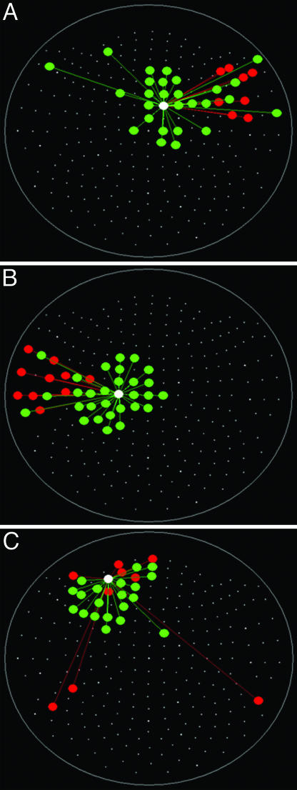
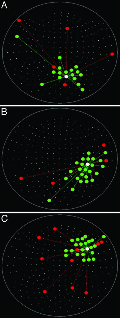
  . Examples of spatial patterns in the distribution of synchronous coupling between a sensor and all other sensors are illustrated in Figs. 1 and 2.
Fig. 1.
Spatial patterns of  for three separate sensors (large white circles). Only statistically significant
  are plotted. The statistical significance threshold was adjusted to account for 247 multiple comparisons per plot, according to the Bonferroni inequality: the nominal significance threshold is P < 0.05, corresponding to an actual threshold used of P < 0.05/247 (i.e., P < 0.0002). Green and red denote positive and negative
  , respectively. Small white dots indicate the location of the 248 sensors, projected on a plane. Data are from one subject.
Fig. 2.
Spatial patterns of  for three more sensors. Conventions are as in Fig. 1. Data are from the same subject.
Relation Between  and Intersensor Distance. Overall,
  varied with the distance, dij, between sensors i and j. In general, sensors closer to each other tended to have positive
  . The average intersensor distance d̄ij for negative
  was 24% longer than for positive
  . Specifically, d̄ij (
 ) was 198.92 ± 0.21 mm (n = 138,700), and d̄ij (
 ) was 160.12 ± 0.24 mm (n = 146,675). Overall, there was a strong and highly significant negative association between
  and the log-transformed dij, ln(dij). The Pearson correlation coefficient between signed
  and ln(dij) was -0.519 (P < 10-20). This relation indicates that the strength of synchronous coupling tended to fall off sharply with intersensor distance.
Synchronous Dynamic Neural Networks. The  is an estimate of synchronous coupling between neuronal populations in which the absolute value and sign of
  denote the strength and kind of coupling, respectively. If the neural ensembles sampled by the 248 sensors are considered nodes in a massively interconnected neural network, then the
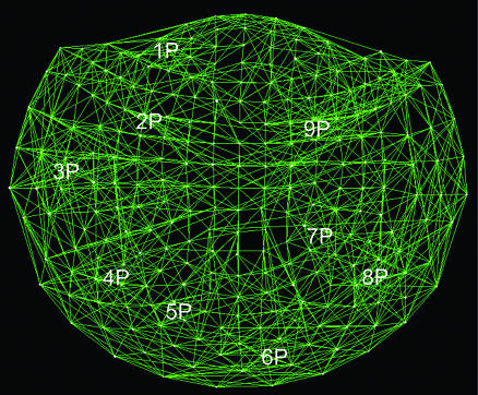
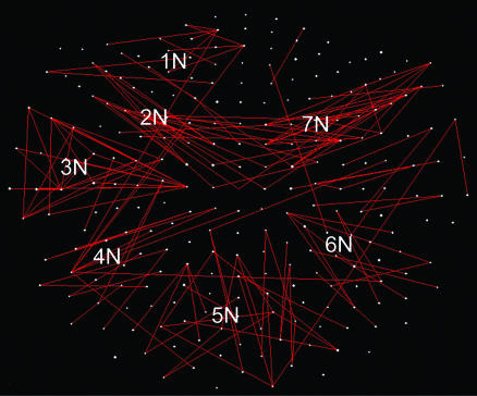
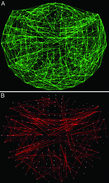
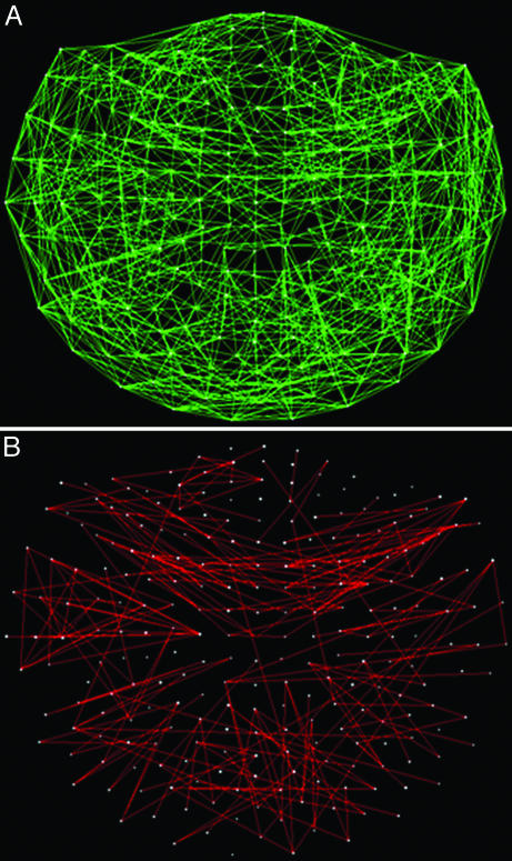
  can serve as an estimate of the dynamic synchronous interactions between these nodes. We visualized such a massively interconnected network by connecting the 248 nodes with green or red lines, denoting positive or negative coupling, respectively. Figs. 3 and 4 show a thresholded and scaled view of this network, averaged across the 10 subjects; regional variations in interactions were present and consistent across subjects (Figs. 5 and 6). There are several interesting features in this network, which follow: (i) most of the next-neighbor interactions are positive; (ii) most of negative interactions occur at longer distances; (iii) interactions with centrally located sensors are relatively sparse; and (iv) interhemispheric interactions are infrequent, probably because of the longer distances involved. In addition, systematic variations in the local density of interactions can be distinguished qualitatively, as follows (in counterclockwise direction). There were nine regions of positive interactions (Fig. 3), consisting of sensors overlying the following brain regions: left anterior-frontal (1P), left dorsal-frontal (2P), left lateral-frontal-temporal (3P), left parietal (4P), left parietal-occipital (5P), right occipital (6P), right parietal-temporal (7P), right temporal (8P), and right frontal (9P). For negative interactions (Fig. 4), seven regions could be distinguished, consisting of sensors overlying the following brain regions: left anterior-frontal cortex (1N), left dorsal-frontal (2N), left lateral-frontal-temporal (3N), left parietal (4N), occipital (5N), right parietal (6N), and right frontal (7N). Several of the positive and negative interactions were spatially overlapping.
Fig. 3.
Massively interconnected network, averaged across the 10 subjects (mean  converted to
  , see Methods). Green denotes positive
  . Numbers in white denote local regions of higher density of interactions. The statistical significance threshold was adjusted to account for 30,628 multiple comparisons (i.e., all possible
  , see text), according to the Bonferroni inequality: the nominal significance threshold is P < 0.001, corresponding to an actual threshold used of P < 0.001/30,628 (i.e., P < 0.00000003).
Fig. 4.
Massively interconnected network, averaged across the 10 subjects (mean  converted to
  , see Methods). Red denotes negative
  . Conventions are as in Fig. 3.
Fig. 5.
Massively interconnected network for an individual subject. Conventions are as in Figs. 3 and 4.
Fig. 6.
Massively interconnected network for a different subject. Conventions are as in Figs. 3 and 4.
Robustness of Network Across Subjects. Remarkably, neural networks constructed as above were very similar across subjects (Figs. 5 and 6). We quantified and assessed overall network similarity between all subject pairs by calculating the Pearson correlation coefficient across all  (i.e., all i and j sensors) of the network. The correlation coefficients obtained were very high and highly significant (median = 0.742; range, 0.663–0.839; P < 10-20 for all correlations; >20,000 degrees of freedom). These findings suggest a common network foundation.
Discussion
This work assessed synchronous dynamic coupling between single-trial MEG time series made stationary by using ARIMA modeling (4). Therefore, the results obtained are valid estimates of this coupling, uncontaminated by nonstationarities typically present in raw MEG data. In this article, we focused on zero-lag cross-correlations, which estimate synchronous coupling between two time series. From these correlations, we then computed partial correlations, which provide an estimate of sign and strength of direct coupling between two sensor series because possible effects mediated indirectly by other sensors are removed. Finally, the  enabled us to construct a synchronous dynamic network in which the sign and strength of the
  served as estimates of the sign and strength of direct neuronal population coupling. In general,
  were smaller than the raw cross-correlations because all other possible 246 associations in the sensor ensemble were accounted for. However, small-amplitude interactions are the rule for stability in massively interconnected networks. For example, in a previous study of such networks (6), the normalized connection strength ranged from -0.5 to 0.5 at the beginning of training of the networks but ranged from approximately -0.2 to 0.2 in the trained, stable network. Comparably, in the present study, the range of
  was similar (-0.19 to 0.36).
 were positive or negative and of various strengths depending on the particular pair of sensors and their distance, such that
  tend to be higher at short distances. It could be argued that this tendency might be due to multiple detectors viewing the same neural sources. Although there is no quantitative measure of this component, our results assure us that it does not dominate the correlation patterns seen. Specifically, the rapid fall of the magnetic field strength with distance, along with the effect of gradiometer coils, would result in a very tight pattern of correlations of signal due to this contribution, with no distant interactions visible on the same scale. Instead, what we see from our analysis are complex patterns of interactions over the entire cortex, visible on a single amplitude scale. It is true that the correlations shown are stronger for near sensors, but neural activity is generally more correlated locally. Finally, the calculation of partial correlations would further eliminate potentially spurious effects.
In previous studies, associations between neuronal ensembles (recorded as EEG, MEG, or local field potentials) have been investigated most often by using frequency-domain (see, e.g., refs. 7–11) or time-domain (see ref. 12 for a review) analyses applied to a whole data set or within specific spectral frequency bands. In such analyses, association measures are commonly calculated from the data without testing for their stationarity (see ref. 10 for an exception). Stationarity (or quasistationarity) is a prerequisite for obtaining accurate measurements of moment-to-moment interactions between time series (as contrasted to shared trends and/or cycles), both in the time domain (by computing cross-correlation) and in the frequency domain (by computing squared coherency) (1–3). Cross-correlation or coherency estimates based on raw nonstationary data yield erroneous estimates and spurious associations.
It should be noted that the sign of cross-correlation does not provide information regarding underlying excitatory or inhibitory synaptic mechanisms but merely indicates the kind of simultaneous covariation with respect to the mean of the series: a positive correlation indicates covariation in the same direction (increase/increase, decrease/decrease), whereas a negative correlation indicates covariation in opposite directions (increase/decrease, decrease/increase). In general,  tended to vary in an orderly fashion in sensor space, such that it tended to be positive between neighboring sensors and negative between sensors farther away. Although this tendency was a significant underlying overall relation, there were clear and distinct exceptions, including negative
  between neighboring sensors and positive
  between far-away sensors. In addition, the spatial
  pattern differed depending on the location of the reference sensor. Altogether, these findings suggest a robust and relationally orderly correlation structure, but with distinct local specificity. Indeed, these characteristics are the fundamental attributes that endow the resulting massively interconnected network with the characteristic structure illustrated in Figs. 3, 4, 5, 6. A cardinal feature of this structure was the partitioning of the overall network into regional variations in the strength of positive or negative interactions. The delineation of these mixed interactions would be the next step in this approach, together with an attempt to localize the interactions in brain space by using, e.g., current-density or beam-forming techniques (13–15). These efforts are worthwhile given the remarkable robustness of the network configuration across subjects. This robustness points to a relatively stable synchronous interaction pattern among neural populations, which can, in turn, serve as a canonical network for assessing dynamic brain function.
Acknowledgments
This study was supported by the Mental Illness and Neuroscience Discovery (MIND) Institute (Albuquerque, NM), the Department of Veterans Affairs, and the American Legion Brain Sciences Chair.
Author contributions: A.C.L. and A.P.G. designed research; F.J.P.L. and A.C.L. performed research; F.J.P.L., A.C.L., and A.P.G. analyzed data; and A.P.G. and F.J.P.L. wrote the paper.
Conflict of interest statement: No conflicts declared.
Abbreviations: MEG, magnetoencephalography; fMRI, functional magnetic resonance imaging; EEG, electroencephalography; ARIMA, autoregressive integrative moving average.
Footnotes
Leuthold, A. C., 33rd Annual Meeting of the Society for Neuroscience, Nov. 8–12, 2003, New Orleans (abstr.).
References
- 1.Box, G. E. P. & Jenkins, G. M. (1970) Time Series Analysis: Forecasting and Control (Holden–Day, San Francisco).
- 2.Jenkins, G. M. & Watts, D. G. (1968) Spectral Analysis and Its Applications (Holden–Day, San Francisco).
- 3.Priestley, M. B. (1981) Spectral Analysis and Time Series (Academic, London).
- 4.Leuthold, A. C., Langheim, F. J. P., Lewis, S. M. & Georgopoulos, A. P. (2005) Exp. Brain Res. 164, 211-222. [DOI] [PubMed] [Google Scholar]
- 5.Snedecor, G. W. & Cochran, W. G. (1989) Statistical Methods (Iowa State Univ. Press, Ames), 8th Ed.
- 6.Lukashin, A. V. & Georgopoulos, A. P. (1994) Neural. Comput. 6, 19-28. [Google Scholar]
- 7.Bressler, S. L. (1995) Brain Res. Rev. 20, 288-304. [DOI] [PubMed] [Google Scholar]
- 8.Mitra, P. P. & Pesaran, B. (1999) Biophys. J. 76, 691-708. [DOI] [PMC free article] [PubMed] [Google Scholar]
- 9.Pfurtscheller, G. & Lopes da Silva, F. H. (1999) Clin. Neurophysiol. 110, 1842-1857. [DOI] [PubMed] [Google Scholar]
- 10.Ding, M., Bressler, S. L., Yang, W. & Liang, H. (2000) Biol. Cybern. 83, 35-45. [DOI] [PubMed] [Google Scholar]
- 11.Astolfi, L, Cincotti, F, Mattia, D., Salinari, S., Babiloni, C., Basilisco, A., Rossini, P. M., Ding, L., Ni, Y., He, B., et al. (2005) Magn. Res. Imaging 22, 1457-1470. [DOI] [PubMed] [Google Scholar]
- 12.Singer, W. (1999) Neuron 24, 49-65. [DOI] [PubMed] [Google Scholar]
- 13.Gorodnitsky, I. F., George, J. S. & Rao, B. D. (1995) Electroencephalogr. Clin. Neurophysiol. 95, 231-251. [DOI] [PubMed] [Google Scholar]
- 14.Uutela, K., Hamalainen, M. & Somersalo, E. (1999) NeuroImage 10, 173-180. [DOI] [PubMed] [Google Scholar]
- 15.Gross, J., Kujala, J., Hamalainen, M., Timmermann, L., Schnitzler, A. & Salmelin, R. (2001) Proc. Natl. Acad. Sci. USA 98, 694-699. [DOI] [PMC free article] [PubMed] [Google Scholar]


