Extending Unbiased Stereology of Brain Ultrastructure to Three-dimensional Volumes

Abstract

Objective: Analysis of brain ultrastructure is needed to reveal how neurons communicate with one another via synapses and how disease processes alter this communication. In the past, such analyses have usually been based on single or paired sections obtained by electron microscopy. Reconstruction from multiple serial sections provides a much needed, richer representation of the three-dimensional organization of the brain. This paper introduces a new reconstruction system and new methods for analyzing in three dimensions the location and ultrastructure of neuronal components, such as synapses, which are distributed non-randomly throughout the brain.

Design and Measurements: Volumes are reconstructed by defining transformations that align the entire area of adjacent sections. Whole-field alignment requires rotation, translation, skew, scaling, and second-order nonlinear deformations. Such transformations are implemented by a linear combination of bivariate polynomials. Computer software for generating transformations based on user input is described. Stereological techniques for assessing structural distributions in reconstructed volumes are the unbiased bricking, disector, unbiased ratio, and per-length counting techniques. A new general method, the fractional counter, is also described. This unbiased technique relies on the counting of fractions of objects contained in a test volume. A volume of brain tissue from stratum radiatum of hippocampal area CA1 is reconstructed and analyzed for synaptic density to demonstrate and compare the techniques.

Results and Conclusion: Reconstruction makes practicable volume-oriented analysis of ultrastructure using such techniques as the unbiased bricking and fractional counter methods. These analysis methods are less sensitive to the section-to-section variations in counts and section thickness, factors that contribute to the inaccuracy of other stereological methods. In addition, volume reconstruction facilitates visualization and modeling of structures and analysis of three-dimensional relationships such as synaptic connectivity.

Information technology has greatly aided visualization and analysis of the nervous system. Computerized scanning-based imaging modalities such as magnetic resonance imaging provide three-dimensional views of the brain down to about 1 mm of resolution. This level of resolution allows regional analyses of brain function but is not sufficient for investigation of intercellular communication at the level of individual neurons.

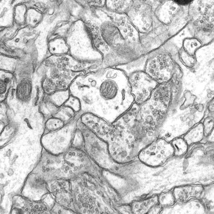
Scanning light microscopy (e.g., confocal microscopy) provides three-dimensional views of individual neurons down to about 1 μm of resolution. Even this higher resolution is not sufficient for visualizing and investigating properties of the tiny connections, called synapses, that occur between neurons. Understanding brain function requires a detailed analysis of connectivity in the brain's neuropil, that region of the gray matter where axons and dendrites from neurons form a dense plexus of synaptic connections. Electron microscopy (EM) is needed for this level of analysis. However, EM requires us to solve the problem of reconstructing a volume from a series of images (see, for example, Figure 10).

Two methods of obtaining a three-dimensional representation of ultrastructure are EM tomography^1,2 and ultrathin serial section EM.^3,4 This paper describes a three-dimensional reconstruction system based on the latter approach, in which parallel sections are cut and imaged separately. The position of each section in the electron microscope introduces rotational and translational offsets. In addition, each section may be exposed to independent amounts of scaling and nonlinear deformation due to cutting, folding, specimen tilt, temperature changes, and optical distortions in the imaging system.⁵ Thus, the image of each section needs to be realigned with the images of adjacent sections.

Early systems for section realignment were often special-purpose optomechanical devices for re-imaging the sections.^4,6,7 In addition to being expensive, these systems corrected only translational and rotational offsets. As computers became more powerful, reconstruction systems began to utilize computer-based registration of images.^8–10 These systems still did not fully correct for nonlinear deformations.³ In the next section of this paper (Volume Reconstruction), we describe an inexpensive system for serial section alignment that corrects for nonlinear deformations, can be applied easily to large images, and requires no special-purpose hardware.

Stereology is the study of three-dimensional distributions of objects from sections. Looking at a sample of parts, stereologists aim to estimate the whole. Having a reconstructed volume of neuropil allows us to go beyond the conventional types of stereological analysis that are performed on ultrastructural distributions. The conventional techniques are almost exclusively based on single or paired sections.^11–14 The one technique that utilizes volumes, the unbiased bricking method, was previously applied to volumes obtained from scanning light microscopes15 but not to large ultrastructural volumes, since such volumes were not easy to generate.

In the Volume Analysis section we describe a number of techniques that are uniquely applicable to volumes of neuropil. We introduce a new, unbiased stereological technique, the fractional counter, and show how it can be applied to the reconstructed volumes as well.

In the last section of this paper (Applications), we demonstrate volume reconstruction of neuropil from stratum radiatum of hippocampal area CA1. We compare the use of the unbiased bricking, disector, and fractional counter techniques in determining synapse density in this volume. In addition, we show how dendrite reconstructions within the sample volume can be used to build surface models for visualization and to obtain an unbiased estimate of the number of spines per unit length of dendrite.

Volume Reconstruction

The volume reconstruction system is embodied in a Windows (2000, 95, 98, and NT) application called serial EM (sEM) Align. The software was developed with the funding of the Human Brain Project and is available online at http://synapses.bu.edu./.

Production and Imaging of Serial Electron Microscopy Sections

Tissue is prepared for serial sectioning and electron microscopy either by intravascular perfusion of fixatives or by microwave-enhanced processing, as detailed elsewhere.^16–18 Microwave-enhanced processing speeds up the penetration of fixatives during immersion and leads to improved tissue preservation for electron microscopy.¹⁹ After processing and embedding, series of about 100 sections are cut at a thickness of 40 to 60 nm on the basis of the observed color of sections. Later, the actual section thickness is estimated, as described below.

Ribbons of sections are mounted on SynapTek pioloform-coated grids (Ted Pella, Inc., Redding, California) and loaded in a rotating stage to facilitate consistent orientation of sections between ribbons. Each series is photographed at the electron microscope onto 3 × 4-inch EM film, typically at 10,000× magnification. A diffraction grating replica grid (0.463 μm per square; Ernest Fullam, Inc., Latham, New York) is photographed at the same time as the series, with the same magnification, for later calibration of image size.

Images are photographed at the microscope rather than digitally imaged directly by a CCD (charge-coupled device) camera, for several reasons. Cooled CCD cameras are expensive and are not as sensitive as film. The integration time for a CCD camera is longer than for film exposure, exacerbating the problem of specimen drift during imaging. Also, the resolution of CCDs is lower than film resolution. A micrograph can be rescanned many times so that different areas can be examined at different magnifications, but direct digital imaging makes it necessary to return to the microscope to reimage a section at each different magnification.

Digitization of sections photographed at the electron microscope can be accomplished in two ways. One way is to print the film onto photographic paper and then scan each print on a conventional flatbed scanner. Another method is to scan the film directly using a high-resolution, large-format film scanner such as the SprintScan45 (Polaroid Corp., Cambridge, Massachusetts) or the AGFA T-2500 (Agfa-Gevaert, Mortsel, Belgium). Scans at 1,000 dpi are sufficient for capturing the details of film photographed at 10,000x magnification. This yields digital images with resolutions of about 400 pixels/μm. At this resolution, the image size of an entire 3 × 4-inch negative is approximately 11 MB. An entire series of 100 sections can be digitally archived in about a gigabyte of storage.

Section Alignment

Transformations

Given a series of digitized images obtained by serial EM, the volume reconstruction problem is to determine a set of transformations {T_i} such that objects in each section are in alignment throughout the volume (Figure 1▶). Each transformation is represented by the functions:

where (u,v) is a pixel of the original image and (x,y) is a pixel of the transformed image. The choice of basis functions {f_j(x,y)} determines the type of adjustments that are possible. A practical choice for {f_j(x,y)} is the set of bivariate polynomials.^8,20 The first three terms,

give the set of all possible linear transformations, which includes translation, rotation, skew, and scaling. Nonlinear transformations that correct for deformations can be made by including second-order terms:

Figure 1.

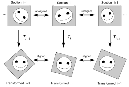
Alignment of serial section images in absolute mode. The original section images (top row) are unaligned. After applying the appropriate transformation (T) to each section image, the resulting transformed section images are all in alignment (bottom row).

This is the set of basis functions implemented in the software and used for all reconstructions described here. The real-valued parameters {a_j}, {b_j}, where j = 0…5, specify the particular transformation for each section. The parameters can be determined by either of two methods —manual adjustments by the user or computation from a set of point correspondences.

Transformations can be utilized in two ways. In absolute mode (Figure 1▶), each transformation places the section into alignment with all the other transformed sections in the series. The stack of transformed sections in absolute mode forms the reconstructed volume. Alternatively, an incremental alignment can be performed in which each transformation aligns the section to the untransformed adjacent section (Figure 2▶). This mode provides a way for section-by-section alignments to be corrected without the need to adjust subsequent sections in the alignment. Also, incremental alignment mitigates problems with persistent drift or scaling introduced by repeated errors in user input. However, incremental alignments must be converted to absolute alignments to form the final reconstructed volume, and this conversion is not exact. (See Converting Incremental to Absolute Forms, below.)

Figure 2.

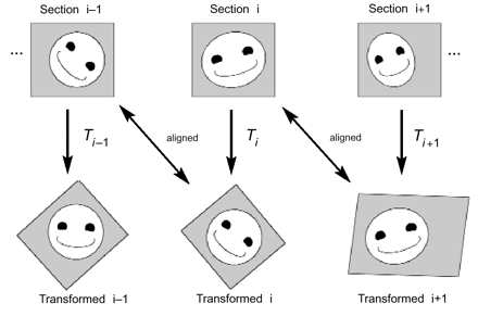
Incremental alignment of serial section images. The original section images (top row) are unaligned. After applying the appropriate transformation (T_i) to section i, the resulting transformed image is in alignment with the original image of section i–1. Likewise, the transformed section i+1 is in alignment with the untransformed section i. Since each alignment is independent of alignments between other sections, incremental alignments allow easy modification of alignments. Ultimately, the incremental alignment is converted to an absolute alignment for analysis.

Point Correspondence Method

Alignments are automated through the use of point correlations.^1,20–22 Transformation parameters are calculated automatically from a set of point correspondences given by the user. This method is less labor intensive than manual adjustments (see User Interface, below) and will work for any choice of basis functions.

In many systems that use point correspondences for alignment, artificial fiducials are introduced prior to sectioning to support the alignment algorithm.²¹ Fortunately, serial EM of neuropil has intrinsic fiducials in the form of cross-sectioned microtubules, mitochondria, and other small, cylindric organelles. The centers of these structures can be used to form a set of point correspondences for alignment.

Given a set of points {(x₀,y₀), (x₁,y₁), (x₂,y₂), …, (x_m,y_m)} in section i-1 and a set of corresponding points {(u₀,v₀), (u₁,v₁), (u₂,v₂), …, (u_m,v_m)} in adjacent section i, the transformed section i is aligned to section i–1 (incremental alignment, Figure 2▶) when

where

and

are the parameters of the desired section i transformation.

The least-squares solution to this equation can be computed by singular value decomposition. Singular value decomposition is robust to underconstrained problems and thus will not be overly sensitive to the choice of correspondence points.²³ An absolute transformation can be computed by using a set of points {(x₀,y₀), (x₁,y₁), (x₂,y₂), …, (x_m,y_m)} from the transformed section i-1 instead.

Converting Incremental to Absolute Forms

To generate an aligned volume, an incremental alignment is converted to an absolute alignment. Since each transformation contains nonlinear terms, composing the transformations section by section poses problems. This is dealt with by numerically approximating the composition using the singular value decomposition computation.

Given an alignment as depicted in Figure 2▶, the following algorithm is used:

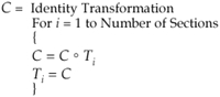
To determine C _° T_i (where “ _° ” denotes composition), start with a set of basis points, such as {(0,0), (w,0), (0,h), (w/2,h), (w,h/2), (w,h)}, where w is the width of the image and h is the height of the image. Map the basis points sequentially through C and then through T_i, yielding a set of corresponding points {(u₀,v₀), (u₁,v₁), (u₂,v₂), …, (u₆,v₆)}. The parameters of the composite transformation are computed using singular value decomposition on these two sets of points, as for the point correspondence method.

User Interface

The software (sEM Align) provides a user interface for viewing the section images, entering correspondence points, making manual adjustments to the alignments, and regenerating the series as an aligned volume. For detailed EM series, each section image will be larger than the PC display size (typically 1024 × 768 pixels). To allow the user to view and align the entire image, it is reduced to fit the display. This reduction is realized by using a predetermined reduction factor and linear filter function of the appropriate width for anti-aliasing.²⁴ Since the user aligns reduced images, nonlinear alignments of arbitrarily large images can be previewed on screen almost instantaneously.

To apply the resulting transformations to the full, unreduced images, new parameters {a′_j} and {b′_j} must be computed. The form of the computation depends on the basis functions. For the bivariate polynomial basis, the transformation parameter correction is realized by

where s is the ratio of the original image size to the reduced image size. The resulting parameters can be modified to new values for a different display size using this formula with the inverse of s.

The user interface also enables the user to manually move an image using keystrokes. The image can be translated, rotated, scaled, skewed, and squeezed (or enlarged) along one edge. To evaluate adjustments on screen, the user compares section images by either of two methods—blending or flickering. Blending displays two overlaid images, each with half the luminance of the original image. Provided that sections are sufficiently thin, blended images become sharper as they align, blurrier as they go out of registration (Figure 3▶). Flickering between two section images produces apparent motion in the direction of offset, which can guide manual adjustments.⁶

Figure 3 .

Blended images from two adjacent serial sections. Left, When sections are in good alignment, objects are clear because object boundaries overlie each other. Right, When sections are misaligned, the image is blurry because of the doubling of object boundaries.

After all sections have been aligned using these techniques and converted to absolute form, the software can apply the transformations to the full (unreduced) images to generate a new set of serial section images. These images make up the digitized volume of neuropil and are suitable for use with other software, such as IGL Trace (also available at http://synapses.bu.edu/), for analysis and three-dimensional surface modeling.

Volume Calibration

The final step in the reconstruction is to calibrate the dimensions of the digitized volume. An image of the calibration grid is digitized at the same resolution as the serial section images to allow calibration of the dimensions in the planes of the sections, the x- and y-directions. Using IGL Trace, a set of lines is drawn on the calibration grid. Each line extends x_i pixels in the x direction and y_i pixels in the y direction. By counting the number of grid squares spanned by a line, its length in microns (l_i) is known. The correct x- and y-calibration factors, c_x and c_y, in microns per pixel, would realize

by the Pythagorean theorem. Thus, c_x and c_y can be determined by minimizing the sum of the squared errors for the calibration lines, i.e., minimizing

The thickness of the volume perpendicular to the planes of the sections is determined by the section thicknesses, which can differ from the nominal value set at the time of slicing. A number of methods have been proposed for estimating the thickness of ultrathin sections,²⁵ none of which are applicable to digitized serial sections. We therefore developed an alternative method that allows the mean section thickness of the entire series to be estimated once the x- and y-calibration factors are known.^16,26

In any series, cylindric objects such as axons, dendrites, and mitochondria will occasionally be sectioned longitudinally. By measuring the width of such a cylinder (d_i) at its central section and then counting the number of sections (s_i) in which it appears, section thickness can be computed as the ratio of these two values (Figure 4▶). The mean section thickness for a series is obtained by averaging the results from a number (N) of such object measurements distributed evenly through the series:

Figure 4.

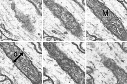
A sequence (from upper left to lower right) of six serial sections that pass longitudinally through a mitochondrion (M). At the central section, the diameter (d) is measured. Since the mitochondrion is cylindric, the ratio of the diameter to the number of sections spanned by the mitochondrion is an estimate of section thickness. On the first and last section, the mitochondrion may appear as a gray wall at the point where the diameter was measured. In such cases, depending on the darkness of the gray wall, a fractional value of either 0.25, 0.5, or 0.75 is used instead of the full section count. For the case shown, the mitochondrion spans four sections fully and about 0.25 sections at either end, for a thickness estimate of d/4.5.

The thickness of the reconstructed volume is the mean section thickness multiplied by the total number of sections.

Volume Analysis

The distributions of ultrastructural objects should be assessed using unbiased stereological counting methods. As a concrete example, suppose a condition was suspected to affect the density of synapses in a brain region, as might be the case following a general loss of synaptic activity²⁷ or potentiation of a particular afferent pathway.¹⁹ Assessment of synapse density requires a three-dimensional sample of tissue; it cannot be done on single sections.^14,28 Reconstructed volumes provide an ideal three-dimensional sample, but because the sample is a small fraction of the whole, care should be taken to avoid biases associated with counting synapses that lie only partly in the sample.

To understand the issues, it is helpful to consider the problem in two dimensions. To determine the density of two-dimensional profiles in an area (A_ref), a grid of sampling frames, each of area A_f, can be superimposed (Figure 5▶, left). This technique is convenient for work at the light microscope, since A_ref can be estimated by counting the number of grid points that contact the area, and profiles can be counted for a random subset of sampling frames.

Figure 5 .

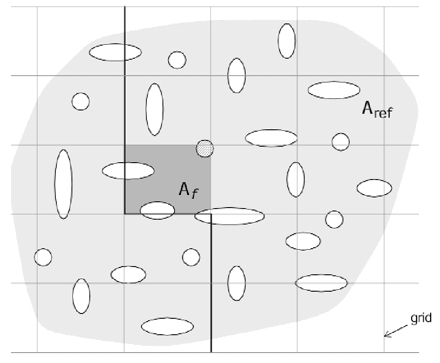
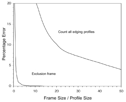
Two-dimensional sampling from a grid of rectangular frames. Left, A grid of two-dimensional sampling frames is placed over an area (A_ref, light gray) containing profiles (white) to be counted. A single sampling frame (A_f, dark gray) of the grid with its exclusion lines (bold). Profiles contacting the frame are counted (hashed profile) unless the profiles contact an exclusion line. Thus, for the shaded frame, only one profile is counted. Right, Bias due to edging profiles. When the extended exclusion lines are not used, there is bias due the profiles that intersect the boundary of the sampling frame. When all edging profiles are counted (upper curve), there is much more error than when profiles intersecting two edges are excluded (lower curve). Curves were generated from the ratio of sampled to frame areas with the assumption of a square frame and circular profiles.²⁹ Frame size refers to the width of the frame square. Profile size can be interpreted as the diameter of a circle needed to contain the largest profile in the reference area.

A problem arises for profiles intersecting the borders of a sampling frame. Should these edging profiles be counted or not? One strategy is to count all edging profiles. When this is done, profiles that lie mostly outside of the sampling frame are included. Profiles that intersect more than one frame will be counted more than once. Another strategy is to count all edging profiles except those that touch the bottom or left edges of the frame. This technique also has some bias that depends on the size of the profiles relative to the size of sampling frame.²⁹ The bias is small, provided that the frame is much larger than the largest profiles (Figure 5▶, right).

Extending the exclusion lines through the reference area (Figure 5▶, left) yields a counting rule that eliminates the remaining bias.²⁹ Profiles that intersect the frame are counted, except for those profiles contacting an exclusion line. Using this approach, the density of profiles in A_ref is estimated by

where Q_f^– is the count from each analyzed frame f, A_f is the area of the frame, and β_f is the fraction of the frame that lies inside A_ref. If every frame in the grid is analyzed, clearly every profile is counted once and only once, and the denominator is equal to A_ref; therefore, the correct N_A is obtained for the reference area.

Unbiased Brick

Extending this concept to three dimensions leads to the unbiased bricking rule.^15,30,31 Previously, this rule could only be applied to microscopes that produced registered volumes,¹⁵ but the ability to reconstruct a volume of neuropil from serial sections using a PC broadens the applicability of the technique. In this approach, three faces of the brick are inclusion faces, and the other three faces lie in exclusion planes (Figure 6▶). Objects wholly inside the brick or touching only inclusion faces are counted, whereas objects touching the exclusion planes anywhere, even outside the faces of the brick, are not counted. This rule gives an unbiased estimate of number per volume:

where Q_b^– is the count obtained and V_b is the volume of each brick. (For simplicity, it is assumed that each brick volume is totally contained in the reference volume.) Notice that, for B number of bricks,

except when all brick volumes V_b are equal. In other words, the correct estimate of number per volume is not obtained by taking the mean of the estimates from each brick.

Figure 6 .

Extension of the sampling frame concept to three dimensions produces a “brick” in the shape of a rectangular prism (dashed outline). The brick is bordered by exclusion planes (labeled “exclude”) on three sides. Objects intersecting the bottom of the brick are excluded, as are objects intersecting the back or left side of the brick. In addition, there are exclusion regions adjacent to the front and top faces of the brick. The top, front, and right side of the brick are inclusion faces. The brick has height h perpendicular to the plane of sectioning.

Disector

In the special case where the height (h) of the brick (Figure 6▶) is always less than the height of any object to be counted, the interior of the brick can be ignored. In this case no object will fit wholly inside the brick, and only objects that touch an inclusion face, but not an exclusion plane, need be counted. This simplified use of unbiased bricking is referred to as the disector technique.³² The density estimate is

where Q_d^– is the count per disector and V_d = h × A_f is the volume of a given disector. Notice that a sequence of disectors between adjacent sections repeated serially through a reconstructed volume is equivalent to the unbiased bricking technique.

Fractional Counter

An alternative but equally unbiased approach to the bricking method can be obtained by considering fractional counts. This is most easily understood first in two dimensions (Figure 7▶). All profiles that intersect a sampling frame are counted according to the fraction of the profile that lies within the frame. For those that are wholly in the frame, the fraction (α) is 1. For those that are not wholly in the frame, the fraction is less than 1. A natural fraction to consider is the fraction of the profile area, but any type of fraction will do so long as the sum of the fractional parts of a profile add up to 1.

Figure 7 .

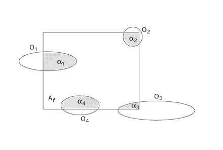
Each object's profile (O_i) has a fraction (α_i) that lies inside a test frame with area A_f. An unbiased estimate of profile density can be computed by counting these fractions.

The equation

is an unbiased estimator of the number of profiles per area. Here, A_T is the total area analyzed, (i.e., Σβ_fA_f, as above,) and the α_j indicates the fractions of the profile areas contained in A_T. Notice that when an entire grid of sampling frames covering the reference area is analyzed, A_T equals A_ref, α_j equals 1 for all j, and no profile is counted more than once.

Generalization of this formula yields the fractional counter in three dimensions:

An unbiased estimate of the number of objects per volume is the sum of fractions (f_o) of all objects (o = 1…n) intersecting the test volumes V_i, divided by the total test volume (V_T = ΣV_i). This can be rewritten

where is the number of objects encountered and f̄_o^– is the mean volume fraction over all objects.

As a practical matter when using the fractional counter in serially sectioned material, it is often easier to determine the fraction in the direction of sectioning rather than in the plane of section. This is because sectioning has already cut the object into parts, and the number of sections in which the object appears is easily assessed to determine object fraction. Determining the fraction in a section requires an imposed measurement, such as the overlay of a fine grid, to determine object fraction. An alternative is to use an unbiased sampling frame (i.e., with exclusion and inclusion lines) to select profiles in the plane while considering fractions only between sections. With this technique, fractional issues in the plane of the sections are eliminated, since a profile is either wholly included in or excluded from a section.

Notice that this estimator does not have particular volume requirements, such as the requirement of a pair of sections for the disector. A single section can be used, provided that the section thickness can be accurately determined (Figure 8▶). In this case the object fraction is

Figure 8 .

A serially sectioned object appears as a single profile (bold ellipse) in the sampling frame (solid and dashed lines) placed into one of the sections. The object also has profiles that appear on adjacent sections (light ellipses). In total, the object has profiles that appear on s_o number of sections. The object fraction within the section is 1/s_o.

The fractional counter then reduces to

where Q^– is the number of objects counted in the sampled section, and s_o is the number of sections spanned by each object. The last term is just the mean object fraction, as before. The volume of each sample is the area of the sample frame times the section thickness.

This special case of the fractional counter for single sections was first proposed by Cruz-Orive³⁰ and has also been used to determine synapse density from serial EM.¹⁹ (In Sorra and Harris,¹⁹ “mean of 1/s_o“ is misprinted as “1/mean of s_o,“ although the correct calculation was used throughout.)

Unbiased Ratios

A potential problem with the above methods is that the volume of the sample enters explicitly into the calculation. Thus, when there are overall changes in volume prior to sampling, (e.g., due to shrinkage or gliosis), the measured density will be accordingly distorted. This problem can be eliminated by considering ratios of objects.³¹ A useful ratio measure is to consider the ratio of different classes of objects. Suppose, for example, object density is measured for all objects {O} and for a subclass of these objects {S}, using unbiased bricking. Then the ratio of S to O is

The ratio method can be used with any of the above unbiased density measures (see, for example, Harris et al.³³ and Sorra et al.³⁴).

Per-length Counting

Another useful measure is the distribution per unit length of dendrite. This measure is applicable because a reconstructed volume contains the dendritic segments that traverse that region of the neuropil. Many neurons have dendritic spines, where most of the excitatory synapses occur. Hence, one desirable quantity is the number of spines per unit length of dendrite.^27,33 In this section we propose a stereological procedure to eliminate bias in these measurements.

A segment of dendrite contained in a set of serial EM sections represents a sample of the total dendrite length. Consider a sequence of such samples, each of length l_i, covering the entire dendrite (Figure 9▶). To estimate spines per length (N_L), the places where the spine neck originates from the shaft are counted. The amount of bias introduced by counting all spine origins that occur anywhere on the segment is proportional to the ratio of the length of the origins to the length of the segment. To avoid over-counting at the boundaries between segments, define an exclusion end and an inclusion end. Spine origins that touch the exclusion end of the segment are not counted. Thus, the estimate is

where q_i^– is the count of spine origins from the ith segment. As with the previous techniques, N_L is equal to the mean of the individual counts per segment if and only if segment lengths l_i are the same for all segments.

Figure 9 .

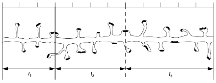
Sampling of a dendrite by a series of test regions of length l_i. Each spine originating from the dendrite has a synapse (black). The hash marks at the top show that l₁ is 3, l₂ is 4, and l₃ is 5 units long. For segment 2, the exclusion end is indicated by a dark line. The other end is the inclusion end (dashed line). Similar left exclusion ends and right inclusion ends are defined (but not shown) for the other segments. Using the counting rule described in the text, segment 1 has five spine origins, segment 2 has nine spine origins, and segment 3 has eight spine origins, so the number of spines per length (N_L) is 22/10. Similarly, segment 1 has five synapses, segment 2 has ten synapses, and segment 3 has nine synapses, so N_L is 24/10.

Synapses per length can be similarly estimated, but in this case enough adjacent sections extending beyond the reconstructed segment should be available to ensure that spines are fully traceable. This is because all synapses on spines that originate from a segment should be included in the count provided the spine origin does not touch the exclusion end. Shaft synapses should be likewise included in the count when they do not touch the exclusion end (Figure 9▶).

Applications

A hippocampal slice taken from a 21-day-old rat and maintained for three hours in vitro was prepared for serial sectioning using our standard procedures.²⁷ A series of 94 sections was photographed on a JEOL 1200EX electron microscope and digitized using the Polaroid SprintScan45 at 1000 dpi. Digitization of images from EM film required five hours of labor.

The sections were then aligned using sEM Align. An absolute alignment was generated by selecting cross-sectioned microtubules and mitochondria as corresponding points. Starting with the central section and working downward, lower sections were successively aligned to higher sections. (One transformed section is shown in Figure 10▶, top.) The process was then repeated for the upper half of the series, working up from the central section. For most sections, linear transformations (rotation, translation, skew, and scaling) were sufficient for alignment, but for 16 of the sections second-order terms were also needed to obtain good alignment of the whole field. Alignment of the series required about eight hours.

Figure 10.

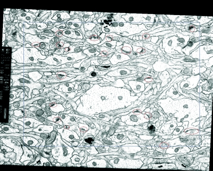
Sample volume reconstruction and analysis. Top, A section of the series showing the sampling frame (blue) and identified synapses (red). The left and top edges of the frame are exclusion edges. A synapse that contacts an exclusion edge is marked with a yellow contour. Bottom, The stack of serial sections for the aligned series is depicted in semi-transparent gray. After alignment, the sections form a volume with an irregular boundary due to the different transformations applied to each section. Inside this irregular volume, a rectangular prism or brick (purple) was defined as a reference volume for making density measurements.

Reference Volume

The alignment resulted in an irregularly shaped volume of reconstructed neuropil (Figure 10▶, bottom). The volume was imported into IGL Trace and calibrated. Using 30 mitochondrial measurements, mean section thickness was estimated to be 0.049 μm. A sampling frame was defined within a section by drawing a rectangular frame using the tracing software (Figure 10▶, top). The edges of the frame were positioned so that the frame never extended beyond the edges of the irregular reconstructed volume on any section. The frame was 7.7 μm by 6.2 μm, for a total area of 47.74 μm². Replicating the frame on every section of the series delineated a rectangular prism of neuropil, the reference volume of 220 μm (Figure 10▶, bottom).

To measure the synaptic density within the reference volume, the volume was treated like an unbiased brick. This provides an unbiased estimate of the overall synaptic density. This reference value can then be compared with the density estimates obtained from smaller samples of the volume using the various methods.

Synapses intersecting the sampling frame in section 1 were marked with a contour using IGL Trace (Figure 10▶, top). Proceeding to section 2, the contours from section 1 were copied into section 2. Any contours that touched the upper or left edge of the sampling frame were marked as excluded. Any contours that belonged to synapses that were not present in section 2 were marked as counted. Then new contours were added for synapses that started on section 2. Proceeding to section 3, the contours from section 2 were copied and all previously counted ones deleted. The remaining contours were then marked as counted or excluded as required. New contours were added for new synapses and the process continued onto section 4. This sequence was continued until all remaining sections were analyzed. Thus, all synapses that ended in the first 93 sections of the series, including those that intersected the first section, were counted. This analysis was completed at a rate of about 20 to 30 sections per hour.

A total of 570 synapses were counted. The last section (section 94) allows the determination of which synapses on section 93 end within the brick, but this last section is not part of the brick volume. Thus, the synaptic density for the reference volume was

Disectors

Each pair of sections analyzed using the procedure just described is a disector. The unbiased bricking analysis on the reference volume consisted of 93 serial disectors, one section thickness in height. Analysis of synaptic density with disectors can be done only with disectors that are a single section thickness in height, because en face synapses, which occur frequently, reside in a single section.³⁵ Of the 570 total synapses, 62 were in only one section.

Another problem with disector analysis on synapses is that perforated synapses can be miscounted. This is because the synapse will appear to end on a section when it is really continued on later sections. Two such synapses were encountered in the reference volume.

The disector has been strongly advocated because of its efficiency, i.e., only a few disectors need to be analyzed to estimate the true density. Practical guides to measuring synaptic density with disectors advise obtaining total counts of 100 to 300.^35,36 In our reconstructed volume, a disector counted, on average, about six synapses. Thus, 33 disectors distributed through the reconstructed volume should be sufficient to accurately estimate synaptic density. So 33 disectors were taken at random from the reference volume (Figure 11▶), giving a density estimate of

Figure 11 .

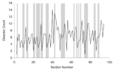
The distribution of disector counts through the reference volume. Each pair of sections in the series represents a disector of one section thickness. The solid line shows the count (Q^–) obtained for each such disector. The gray bars show the random selection of 33 of the disectors for estimation of synaptic density.

Notice, however, that there is a high variance in the number of synapses counted by each disector (Figure 11▶). Disectors that count few synapses are typically followed in the series by disectors that count many synapses, giving a high-frequency oscillation to the distribution of disector counts. This is not a real variation in synaptic density but rather an artifact of the exclusion/inclusion principle operating on small sample volumes. In a worst-case scenario, 33 disectors distributed randomly through the reference volume would count only 118 synapses, giving a density estimate (N_V) of 153/100 μm³. Therefore, with random sampling of single disectors, an underestimate of as much as 42 percent is possible, even when more than 100 synapses are counted!

Unbiased Bricks

Given the systematic variance observed with serial disectors, it is better to use a continuous block of serial disectors (that is, an unbiased brick) than to select them either randomly or at systematic intervals from a series.¹² In addition, with volume reconstruction and IGL Trace, it is actually more efficient to consider contiguous sections than separate disectors since time is saved by copying contours from adjacent sections. To use about the same size sample, density was estimated from four non-overlapping unbiased bricks of eight sections each, starting at sections 12, 34, 56, and 78:

The result is an estimate of density in the reference volume that is more accurate than the estimate obtained with random disectors.

Fractional Counters

For comparison, these same bricks were analyzed using a special case of the fractional counter. All synapses intersecting a brick volume were identified. If the synapses intersected the exclusion edges of the two-dimensional sampling frame in any section, they were not counted.

The remaining synapses were identified completely through all the serial sections in which they resided. The object fraction was computed as the number of sections of the synapse within the brick volume divided by the total number of sections the synapse occupied. These fractions were then summed to give a total fractional count for each brick. The density estimate from fractional counting was thus

The use of fractional counting on the brick volumes improved the accuracy of the estimate at the expense of more work per brick. For this analysis, every synapse that intersected the brick volume had to be uniquely identified in every section it appeared. A total of 254 synapses were thus examined, compared with 198 for the unbiased bricking. Fractional counting on each brick took one to two hours.

With unbiased brick counting, accuracy of the estimate decreases as the brick size decreases. In the limit, the smallest bricks are the disectors, which exhibit large variance (Figure 11▶). Fractional counting on these small volumes reduces this variance. Fractional counts on the 32 single sections in the four bricks just analyzed had a variance of only 2.32, compared with a variance of 7.32 for the disectors on the same sections. The sums of the squared differences of these single-section values from the mean number of synapses per section for the reference volume were 72 for fractional counting and 227 for disectors. Thus, fractional counting has better accuracy than unbiased brick counting, especially for small volumes.

Per-unit-length Counting

Volume reconstruction also facilitates the reconstruction of individual dendrites and the computation of per-unit-length measurements. To illustrate, 20 candidate dendrites with diameters less than 1 μm were selected on a central section. Then, each candidate was reconstructed by tracing the outline of the dendrite and all its spines on each section in sequence. A candidate dendrite was discarded from further analysis if it turned out to be unsuitable for tracing—because it traversed off the side of the reconstructed volume, for example, or was not, in fact, a dendrite at all. Using this approach, 11 of the 20 candidate dendrites were fully reconstructed by tracing their outline with IGL Trace (Figure 12▶). Surface reconstruction of each dendrite and all its protrusions required about two hours of labor.

Figure 12 .

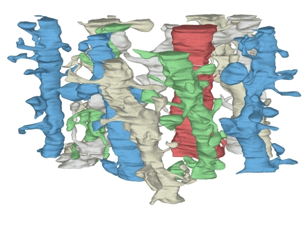
The set of 11 dendrite segments reconstructed from the volume. The dendrites appear in the three-dimensional configuration that they have in the reconstructed volume. They are colored to help distinguish the individual segments and their spines. The red dendrite is a segment from an interneuron as determined by the frequency and clustering of shaft synapses and the lack of mature-looking spines.

By examining dendrites through the series, one of the dendrites was identified as an interneuron by the high density of shaft synapses located along its length. This dendrite was excluded from further analysis, since only pyramidal cell dendrites were to be considered. Notice, however, that the synapses on this interneuron were included in the density measurements described above. Disectors or small brick volumes would have made it impossible to eliminate interneuron synapses from such analysis, perhaps biasing an analysis of the frequency of shaft synapses on pyramidal cells.

Spine-per-length counting was performed on the remaining ten dendrites (Table 1▶). The total length of the reconstructed dendritic segments was 49.5 μm. The number of spine origins were counted, excluding those that intersected section 1 and including those that intersected section 94. Thus, the spine density on the reconstructed dendrites could be computed as

Table 1 ▪.

Results of Reconstruction and Measurement of Ten Dendritic Segments

Dendritic Segment	Length (li) in microns (μm)	Count of Origins (qi-)
D1	4.794	14
D3	5.144	15
D5	4.868	15
D6	4.654	17
D7	4.678	17
D10	4.631	15
D12	5.123	15
D15	4.738	10
D18	5.057	15
D20	5.834	15

Conclusion

Information technology is making three-dimensional analysis of brain ultrastructure increasingly practical. Relatively large volumes of neuropil can be easily reconstructed from serial EM in just a couple of days work by using our PC software. The reconstructed volumes offer several advantages for analyzing synaptic neuropil and complex ultrastructure. Most important, since all objects are in alignment they can be easily identified from section to section. This ability to unequivocally identify serial-sectioned profiles as belonging to the same three-dimensional object is a fundamental requirement of all stereological techniques.^31,37 Excluding objects that cannot be clearly identified in a single section violates this basic requirement. Often, a quick examination through adjacent serial sections is sufficient to identify the objects.

Working with volumes rather than single sections is important for other reasons as well. Many organelles, such as synapses³⁸ and smooth endoplasmic reticulum,³⁹ have complex shapes that cannot be adequately described or understood without a three-dimensional view. Volume reconstruction aids the analysis of connectivity relationships, such as the source of the postsynaptic partners of a multi-synaptic bouton^40–42 or the relationships among presynaptic partners of branched spines.³⁴ In addition, volume reconstruction facilitates exclusion of objects that are not of interest. For example, by reconstructing dendritic segments, dendrite types can be identified and shaft synapses on non-spiny dendrites of interneurons can be excluded from synapse counts intended to represent spiny neurons only.

Reconstruction of volumes of neuropil makes volume-oriented analysis methods, such as the unbiased brick and fractional counter methods, practicable. These methods capture a larger sample of the object distribution, thus avoiding the systematic section-to-section variations that contribute to the inaccuracy of other methods. Volume-oriented analyses are less sensitive to section-to-section variations in section thickness. Average section thicknesses, which are easier to compute from digitized sections, are more applicable to the volume methods.

Synapse density is one type of ultrastructural analysis that is frequently performed in neuroscience.^{12,19,33,35,36} On the basis of our results, we propose the following general rules for performing synaptic density analysis on reconstructed volumes:

• Reconstruct a large field but use sufficient magnification to allow clear identifications.

• Choose a large sampling frame size relative to the size of synapses to minimize inadvertent biases associated with two-dimensional exclusion and inclusion of profiles.

• Use sampling bricks with large numbers of continuous sections to improve accuracy and minimize inadvertent biases associated with sampling through serial sections.

For very large volumes, both the fractional counter and unbiased bricking methods will produce similar results. However, if the sampling frame is small or few sections are analyzed, use fractional counting to reduce variance and improve accuracy.

References

- 1.Jing Z, Sachs F. Alignment of tomographic projections using an incomplete set of fiducial markers. Ultramicroscopy. 1991;35:37–43. [DOI] [PubMed] [Google Scholar]
- 2.Soto GE, Young SJ, Martone ME, et al. Serial section electron tomography: a method for three-dimensional reconstruction of large structures. Neuroimage. 1994;1:230–43. [DOI] [PubMed] [Google Scholar]
- 3.Huijsmans DP, Lamers WH, Los JA, Strackee J. Toward computerized morphometric facilities: a review of 58 software packages for computer-aided three-dimensional reconstruction, quantification, and picture generation from parallel serial sections. Anat Rec. 1986;216:449–70. [DOI] [PubMed] [Google Scholar]
- 4.Stevens JK, Davis TL, Freidman N, Sterling P. A systematic approach to reconstructing microcircuitry by electron microscopy of serial sections. Brain Res Rev. 1980;2:265–93. [DOI] [PubMed] [Google Scholar]
- 5.Stevens JK, Trogadis J. Computer-assisted reconstruction from serial electron micrographs: a tool for the systematic study of neuronal form and function. Adv Cell Neurobiol. 1984;5:341–69. [Google Scholar]
- 6.Levinthal C, Ware R. Three-dimensional reconstruction from serial sections. Nature. 1972;236:207–10. [Google Scholar]
- 7.Pearlstein RA, Kirschner L, Simons J, Machell S, White WF, Sidman RL. A multimodel system for reconstruction and quantification of neurological structure. Anal Quant Cytol. 1986;8(2):108–15. [PubMed] [Google Scholar]
- 8.Brown LG. A survey of image registration techniques. ACM Comput Surv. 1992;24(4):325–76. [Google Scholar]
- 9.Toga AW, Banerjee PK. Registration revisited. J Neurosci Methods. 1993;48:1–13. [DOI] [PubMed] [Google Scholar]
- 10.Van den Elsen PA, Pol E-JD, Viergever MA. Medical image matching: a review with classification. IEEE Eng Med Biol. 1993;12:26–9. [Google Scholar]
- 11.Coggeshall RE, LaForte R, Klein CM. Calibration of methods for determining numbers of dorsal root ganglion cells. J Neurosci Methods. 1990;35:187–94. [DOI] [PubMed] [Google Scholar]
- 12.Coggeshall RE, Lekan HA. Methods for determining numbers of cells and synapses: a case for more uniform standards of review. J Comp Neurol. 1996;364:6–15. [DOI] [PubMed] [Google Scholar]
- 13.Cruz-Orive LM. Stereology of single objects. J Microsc. 1997;186:93–107. [Google Scholar]
- 14.Howard CV, Reed MG. Unbiased Stereology: Three-dimensional Measurement in Microscopy. New York: Springer, 1998.
- 15.Howard V, Reid S, Baddeley A, Boyde A. Unbiased estimation of particle density in the tandem scanning reflected light microscope. J Microsc. 1985,138:203–12. [DOI] [PubMed] [Google Scholar]
- 16.Harris KM, Stevens JK. Dendritic spines of CA1 pyramidal cells in the rat hippocampus: serial electron microscopy with reference to their biophysical characteristics. J Neurosci. 1989;9(8):2982–97. [DOI] [PMC free article] [PubMed] [Google Scholar]
- 17.Jensen FE, Harris KM. Preservation of neuronal ultrastructure in hippocampal slices using rapid microwave-enhanced fixation. J Neurosci Methods. 1989;29:217–30. [DOI] [PubMed] [Google Scholar]
- 18.Feinberg MD, Szumowski KM, Harris KM. Microwave fixation of rat hippocampal slices. In: Giberson, Demaree, Microwave Protocols for Microscopy. In press.
- 19.Sorra KE, Harris KM. Stability in synapse number and size at 2 hr after long-term potentiation in hippocampal area CA1. J Neurosci. 1998;18(2):658–71. [DOI] [PMC free article] [PubMed] [Google Scholar]
- 20.Singh M, Frei W, Shibata T, Huth GC, Telfer NE. A digital technique for accurate change detection in nuclear medical images with application to myocardial perfusion studies using thallium-201. IEEE Trans Nucl Sci. 1979;26(1):565–75. [Google Scholar]
- 21.Chawla SD, Glass L, Freiwald S, Proctor JW. An interactive computer graphic system for 3-D stereoscopic reconstruction from serial sections: analysis of metastatic growth. Comput Biol Med. 1982;12(3):223–32. [DOI] [PubMed] [Google Scholar]
- 22.Lawrence MC. Least-squares method of alignment using markers. In: Frank J, Electron Tomography: Three-dimensional Imaging with the Transmission Electron Microscope. New York: Plenum Press, 1992:9–213.
- 23.Press WH, Teukolsky SA, Vetterling WT, Flannery BP. Numerical Recipes in C. Cambridge, UK: Cambridge University Press, 1992.
- 24.Schumacher D. General filtered image rescaling. In: Kirk D. Graphics Gems III. Boston, Mass: Academic Press, 1995: 8–16.
- 25.De Groot DMG. Comparison of methods for the estimation of the thickness of ultrathin tissue sections. J Microsc. 1988;51:23–42. [DOI] [PubMed] [Google Scholar]
- 26.Harris KM, Stevens JK. Study of dendritic spines by serial electron microscopy and three-dimensional reconstructions. In: Lasek RJ, Black MM. Intrinsic Determinants of Neuronal Form and Function. New York: Alan R Liss, 1987;179–99.
- 27.Kirov SA, Sorra KE, Harris KM. Slices have more synapses than perfusion-fixed hippocampus from both young and mature rats. J Neurosci. 1999;19(8):2876–86. [DOI] [PMC free article] [PubMed] [Google Scholar]
- 28.Cruz-Orive LM. Particle number can be estimated using a disector of unknown thickness: the selector. J Microsc. 1986; 145:121–42. [PubMed] [Google Scholar]
- 29.Gundersen HJG. Notes of the estimation of the numerical density of arbitrary profiles: the edge effect. J Microsc. 1977; 111:219–23. [Google Scholar]
- 30.Cruz-Orive LM. On the estimation of particle number. J Microsc. 1980;120:15–27. [DOI] [PubMed] [Google Scholar]
- 31.Gundersen HJG. Stereology of arbitrary particles: a review of unbiased number and size estimators and the presentation of some new ones, in memory of William R. Thompson. J Microsc. 1986;143:3–45. [PubMed] [Google Scholar]
- 32.Sterio DC. The unbiased estimation of number and sizes of arbitrary particles using the disector. J Microsc. 1984;134: 127–36. [DOI] [PubMed] [Google Scholar]
- 33.Harris KM, Jensen FE, Tsao B. Three-dimensional structure of dendritic spines and synapses in rat hippocampus (CA1) at postnatal day 15 and adult ages: implications for the maturation of synaptic physiology and long-term potentiation. J Neurosci. 1992;12(7):2685–705. [DOI] [PMC free article] [PubMed] [Google Scholar]
- 34.Sorra KE, Fiala JC, Harris KM. Critical assessment of the involvement of perforations, spinules, and spine branching in hippocampal synapse formation. J Comp Neurol. 1998;398:225–40. [PubMed] [Google Scholar]
- 35.Geinisman Y, Gundersen HJG, Van Der Zee E, West MJ. Unbiased stereological estimation of the total number of synapses in a brain region. J Neurocytol. 1996;25:805–19. [DOI] [PubMed] [Google Scholar]
- 36.West MJ. Stereological methods for estimating the total number of neurons and synapses: issues of precision and bias. Trends Neurosci. 1999;22:51–61. [DOI] [PubMed] [Google Scholar]
- 37.Cruz-Orive LM, Weibel ER. Recent stereological methods for cell biology: a brief survey. Am J Physiol. 1990;258:L148–56. [DOI] [PubMed] [Google Scholar]
- 38.Spacek J, Harris KM. Three-dimensional organization of cell adhesion junctions at synapses and dendritic spines in area CA1 of the rat hippocampus. J Comp Neurol. 1998;393:58–68. [DOI] [PubMed] [Google Scholar]
- 39.Spacek J, Harris KM. Three-dimensional organization of smooth endoplasmic reticulum in hippocampal CA1 dendrites and dendritic spines of the immature and mature rat. J Neurosci. 1997;17(1):190–203. [DOI] [PMC free article] [PubMed] [Google Scholar]
- 40.Sorra KE, Harris KM. Occurrence and three-dimensional structure of multiple synapses between individual radiatum axons and their target pyramidal cells in hippocampal area CA1. J Neurosci. 1993;13(9):3736–48. [DOI] [PMC free article] [PubMed] [Google Scholar]
- 41.Toni N, Buchs P-A, Nikonenko I, Bron CR, Muller D. LTP promotes formation of multiple spine synapses between a single axon terminal and a dendrite. Nature. 1999;402:421–5. [DOI] [PubMed] [Google Scholar]
- 42.Harris KM. How multiple-synapse boutons could preserve input specficity during an interneuronal spread of LTP. Trends Neurosci. 1995;18:365–9. [DOI] [PubMed] [Google Scholar]