A Diffusion Model Analysis of the Effects of Aging on Letter Discrimination

Abstract

The effects of aging on accuracy and response time were examined in a letter discrimination experiment with young and older subjects. Results showed that older subjects (ages 60–75) were generally slower and less accurate than young subjects. R. Ratcliff’s (1978) diffusion model was fit to the data, and it provided a good account of response times, their distributions, and response accuracy. The results produce similar age effects on the nondecision components of response time (about 50 ms slowing) and the response criteria (more conservative settings) to those from R. Ratcliff, A. Thapar, and G. McKoon (2001), but also show a reduced rate of accumulation of evidence for older subjects. The model-based approach has the advantage of allowing the separation of aging effects on different components of processing.

Investigations of age-related differences in cognitive tasks have often revealed a pattern of declining performance with advancing age. The most dominant hypothesis has been the generalized slowing hypothesis, which states that all information processing is similarly affected by age (e.g., Birren, 1965; Brinley, 1965; Cerella, 1985, 1990, 1991, 1994; Fisk & Warr, 1996; Salthouse, 1985, 1996; Salthouse, Kausler, & Saults, 1988). For some researchers, the general slowing hypothesis has been replaced by one that argues that different task domains show different degrees of slowing, for example, verbal versus spatial domains (see Allen, Ashcraft, & Weber, 1992; Allen, Madden, Weber, & Groth, 1993; Cerella, 1985, 1994; Hartley, 1992; Hertzog, 1992; Lima, Hale, & Myerson, 1991; Madden, 1989; Madden, Pierce, & Allen, 1992; Myerson, Ferraro, Hale, & Lima, 1992; Myerson, Wagstaff, & Hale, 1994; Perfect, 1994; Sliwinski & Hall, 1998). Whether general or domain specific, the slowing hypothesis has been favored by many cognitive aging researchers because it provides a relatively simple and intuitively appealing explanation of age-related decrements across a variety of laboratory tasks and everyday behaviors.

A major source of support for the slowing hypothesis is the empirical regularity observed in Brinley functions. In a Brinley function, older subjects’ response times are plotted against young subjects’ response times and the result is almost always a straight line with a slope in the range of about 1.5 to 2.5 (Brinley, 1965; Cerella, 1985, 1991, 1994; Faust, Balota, Spieler, & Ferraro, 1999; Fisher & Glaser, 1996; Fisk & Fisher, 1994; Hale & Jansen, 1994; Hale, Myerson, & Wagstaff, 1987; Maylor & Rabbitt, 1994; McDowd & Craik, 1988; Myerson & Hale, 1993; Myerson, Hale, Wagstaff, Poon, & Smith, 1990; Myerson et al., 1994; Nebes & Madden, 1988; Perfect, 1994; Salthouse, 1991, chap. 8; Salthouse & Somberg, 1982; G.A. Smith, Poon, Hale, & Myerson, 1988; Spieler, Balota, & Faust, 1996). The slope is taken to be a multiplicative factor that indicates the amount of slowing for the older adults relative to the young adults.

The slowing hypothesis has been challenged, however, on several grounds. First, Fisher and Glaser (1996) have shown that models that distinguish among different components of cognitive processing with different slowing rates can give rise to the regularity of slopes greater than one found in Brinley functions (e.g., Fisher & Glaser, 1996). Second, there has been a new interpretation of what Brinley functions represent. Ratcliff, Spieler, and McKoon (2000) showed that the slope of a Brinley function measures how slow older adults are relative to young adults only under limited types of models. More generally, Brinley functions should be viewed as plots of quantiles against quantiles of the distributions of mean response times across experimental conditions, where the quantiles of a distribution are the points that divide the total frequency in the distribution into parts (e.g., the three quartile points divide the distribution into quarters, the .25, .50, and .75 quantiles). As long as the distributions of mean response times have at least approximately the same shape for the older adults as for the young adults, two results follow: First, the Brinley function is linear, and second, the function’s slope is the ratio of the standard deviations of the older subjects’ and the young subjects’ mean response times. Myerson, Adams, Hale, and Jenkins (2003) claimed that the slope is not the ratio of the standard deviations, rather it is the ratio of the standard deviations multiplied by the correlation coefficient, but this is not correct. The analysis of Brinley functions in terms of quantiles is not a special case of linear regression, as we discuss below. Also, as Ratcliff, Spieler, and McKoon (2003) pointed out, the slope of a Brinley function should not be estimated from linear regression because there is variability (i.e., measurement error) in both the older subjects’ mean response times and the young subjects’ mean response times (see also Draper & Smith, 1998).

Another important point made by Ratcliff et al. (2000) is that the data on which Brinley function analyses are based, mean response times for correct responses, are only a small subset of the data that need to be addressed. Developing a theory based only on mean response time guarantees that the theory will be wrong (or at least inadequate) when applied to other aspects of the data. Dealing with all of the aspects of response time data, namely, correct and error response times and their relative speeds, the shapes of response time distributions for both correct and error responses, and accuracy values, requires an explicit, fully specified quantitative model. Moreover, given such a model, the Brinley function regularity in slope can be produced in multiple ways. For Ratcliff’s diffusion model (Ratcliff, 1978, 1981, 1985, 1988; Ratcliff, Gomez, & McKoon, in press; Ratcliff & Rouder, 1998, 2000; Ratcliff, Van Zandt, & McKoon, 1999), for example, Ratcliff et al. (2000) showed that a slope in the range of 1.5 to 2.5 can be due to, among other possibilities, older subjects adopting more conservative response criteria than young subjects, older subjects accumulating stimulus information more slowly than young subjects, or older subjects having slower response execution processes than young subjects. Crucially, within the framework of the diffusion model (and almost certainly other sequential sampling models, see Ratcliff & Smith, in press), the effects of aging on response times do not map onto standard slowing hypotheses.

Ratcliff’s diffusion model is attractive because it has been successful in accounting for the data from a variety of two-choice response time tasks and because it allows response time data to be analyzed in terms of the components of processing required by a cognitive task. In the aging research domain, Ratcliff, Thapar, and McKoon (2001) applied the model to two visual signal detection tasks, a numerosity judgment task and a distance judgment task. In the numerosity judgment task, subjects viewed an array of asterisks on a computer screen and were asked to decide whether the number of asterisks presented in the display was high or low. In the distance judgment task, subjects viewed two dots and were asked to decide whether the distance between the two dots was large or small. In both tasks, the measures of interest were accuracy, response times for correct and error responses, and the shapes of the response time distributions. For all of these measures, the model gave a good account. The main components of processing into which the model divides the decision process are the quality of the information from a stimulus that drives the decision process, the variability in the quality of the information, the criterial boundaries on the amount of information that must be accumulated in order for a decision to be made, and the nondecisional (encoding and response execution) parts of response time. Applying the model to the numerosity and distance judgment tasks, Ratcliff et al. (2001) identified three main components of comparison between older adults and young adults. First, the older adults set more conservative criteria than the young adults, accumulating more information before making a response. Second, the nondecisional components of processing were slower for the older adults. Third, and most important, the quality of the information driving the decision process was never poorer for the older subjects than the young subjects, and it was sometimes better. This third finding shows that there was no general decrement across all of the components of processing for the older subjects, as the slowing hypothesis predicts there should be.

In the tasks used by Ratcliff et al. (2001), the stimuli were displayed until a response was made, so there was no limit on the time available to encode the stimuli, that is, there was no limit on the availability of perceptual information. The aim of the experiment we report in this article was to extend the diffusion model’s analysis of the components of processing to two-choice decisions for which perceptual information is limited by masking and for which there is good evidence that aging affects the acquisition of stimulus information.

On each trial of the experiment, one of two letters was displayed, then masked, and the subject’s task was to indicate which of the two letters had been presented. Earlier research on visual information processing and backward masking with older adults has suggested performance deficits for older adults in whole versus partial report procedures (Coyne, Burger, Berry, & Botwinick, 1987; Walsh & Prasse, 1980), in visual persistence (; Kline & Nestor, 1977; Kline & Orme-Rogers, 1978; but see Walsh & Thompson, 1978), and in backward masking (Till & Franklin, 1981; Walsh, 1976). Two relatively recent chapters that provide more general reviews of visual deficits in aging are those by Fozard (1990) and Spear (1993). For letter identification specifically, older adults require more time to view a stimulus before it is masked than do young adults in order to reach a criterion level of accuracy in identification (Cramer, Kietzman, & Van Laer, 1982; Hertzog, Williams, & Walsh, 1976; Schlapfer, Groner, Lavoyer, & Fisch, 1991; Till & Franklin, 1981; Walsh, 1976; Walsh, Till, & Williams, 1978; Walsh, Williams, & Hertzog, 1979). The question for the experiment we present was which of the processing components identified by the diffusion model is responsible for the decrement in performance.

The Diffusion Model

The diffusion model is designed to apply only to relatively fast two-choice decisions and only to decisions that are composed of a single-stage decision process (as opposed to the multiple-stage decision processes that might be involved in, for example, reasoning tasks or card sorting tasks). As a rule of thumb, the model would not be applied to experiments in which mean response times are much slower than about 1 to 1.5 s. Models of the general class of diffusion models have also been applied to decision making (Busemeyer & Townsend, 1993; Roe, Busemeyer, & Townsend, 2001) and simple response time (P.L. Smith, 1995).

The diffusion model assumes that decisions are made by a noisy process that accumulates information over time from a starting point toward one of two response criteria or boundaries, as in Figure 1 where the starting point is labeled z and the boundaries are labeled a and 0. When one of the boundaries is reached, a response is initiated. The rate of accumulation of information is called drift rate (v), and it is determined by the quality of the information extracted from the stimulus. For example, if the letter A was displayed for a long time prior to masking, information quality would be good and the mean value of the drift rate toward the A boundary would be large. Within each trial, there is noise (variability) in the process of accumulating information so that processes with the same mean drift rate terminate at different times (producing response time distributions) and sometimes at different response boundaries (producing errors). This source of variability is called within-trial variability. The top panel in Figure 1 shows three processes, all with the same mean drift rate toward the A boundary (shown by the arrow labeled Drift Rate). One terminates quickly at the correct boundary, another terminates more slowly, and the third terminates at the incorrect boundary.

Figure 1.

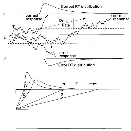
An illustration of the diffusion model. The top panel shows three sample paths (derived from a random walk approximation to the diffusion process) and the effect of moving the boundaries from the solid lines to the dotted lines (where the processes terminate at the points marked T). The bottom panel illustrates the effect on response time (RT) distributions of reducing the drift rate for the fastest and slowest finishing processes by the same amount, X. The fastest responses slow by Y, and the slowest responses slow by Z, which means that longer mean response times result mainly from the distribution skewing.

In the experiment we present, subjects are sometimes instructed to respond as quickly as possible and sometimes to respond as accurately as possible. Speed–accuracy tradeoffs are modeled by altering the boundaries of the decision process—wider boundaries require more information before a decision can be made, and this leads to more accurate and slower responses. The dashed lines in the top panel of Figure 1 show narrow boundaries. With these boundaries, the processes terminate at the points labeled T, one with a correct response and the other two with error responses.

Empirical response time distributions are positively skewed and become more skewed as drift rate decreases. The diffusion model naturally predicts this shape by simple geometry, as shown in the bottom panel of Figure 1. Moving from left to right in the figure, equal size decreases in the rate of approach to the boundary (the X values, shown by the arrows) for the fastest processes lead to smaller increases in response time than those for the slowest processes (shown by the values Y and Z, respectively).

In the diffusion model, the relative speeds of correct and error responses come from variability in processing across trials. Both the drift rate for a stimulus and the starting point for the accumulation of information vary around their means across trials. Panel A of Figure 2 shows the mean drift rates for two letter stimuli (v₋ and v₊) and the distributions of variability for them. Panel B of Figure 2 illustrates the effect of variability in drift rate, using two values of drift rate (v₁ and v₂, symmetrical about v₊, in the top panel) rather than the whole distribution of drift rates that would be used in a real implementation of the model (we assume a normal distribution with standard deviation η). Because the larger drift rate (v₁) produces fast error response times but fewer of them than the smaller drift rate (v₂), the weighted average response time for errors is longer than the weighted average for correct responses. Panel C of Figure 2 shows the effect of variability in starting point, again using two values (z₁ and a − z₁) for illustrative purposes instead of a whole distribution (we assume a uniform distribution with range s_z). When the starting point is near the error boundary, the decision process hits it quickly and with high probability, whereas when it is nearer the correct boundary, errors occur with low probability and they are slow. The weighted average leads to faster error responses than correct responses. The combination of across-trial variability in drift rate and variability in starting point leads to one of three patterns of results: errors faster than correct responses if starting point variability is large, errors slower than correct responses if drift variability is large, and a crossover such that errors at intermediate levels of accuracy (e.g., .5 to .9) are slower than correct responses, and errors at extreme levels of accuracy (e.g., above .95) are faster than correct responses, if both kinds of variability have moderate to large values.

Figure 2.

An illustration of how parameter variability in the diffusion model leads to fast and slow error responses. Panel A shows distributions of drift rate across trials. Panel B shows two processes with drift rates v₁ and f and starting point halfway between the two boundaries. Correct and error responses have equal mean response times (RTs; 400 ms and 600 ms, respectively). The average of these weighted by probability of response leads to slow error responses relative to correct responses. Panel C shows the effect of variability in starting point. Processes starting at z₁ hit the correct boundary with high accuracy and short RT, and errors are slow. Processes starting at a − z₁ hit the correct boundary with lower accuracy and longer RT, and errors are fast. The weighted average gives fast errors relative to correct responses.

Besides the decision process, there are nondecision components of processing such as encoding and response execution. These are combined in the diffusion model into one parameter, T_er (which is not shown in Figures 1 and 2). Like drift rate and starting point, the nondecision components of processing have variability across trials (from a uniform distribution with range s_t). The effect of this variability depends on the mean value of drift rate (Ratcliff & Tuerlinckx, 2002). With a large value of mean drift rate, variability in the nondecision component of processing acts to shift the leading edge of the response time distribution shorter than it would otherwise be (by as much as 10% of s_t). With smaller values of drift rate, the effect is smaller. With variability in the nondecision component of processing, Ratcliff and Tuerlinckx showed that the diffusion model could fit data with large differences in .1 quantile response times across experimental conditions.

In sum, the parameters of the diffusion model correspond to the components of the decision process as follows: z is the starting point of the accumulation of evidence; a is the upper boundary, and the lower boundary is set to 0. For the fits of the model to the data described in this article, the boundaries were assumed to be symmetric about the starting point so that z = a/2. The amount of variability in the mean drift rate across trials is assumed to be normally distributed with standard deviation η and the variability in starting point is assumed to have a uniform distribution with range s_z. For each different stimulus condition in an experiment, it is assumed that the rate of accumulation of evidence is different and so each has a different value of drift, v. Within-trial variability in drift rate (s) is a scaling parameter for the diffusion process (i.e., if it were doubled, other parameters could be doubled to produce exactly the same fits of the model to data). T_er represents the nondecision components of response time, and variability in this across trials is assumed to have a uniform distribution with range s_t.

The components of the model that are the most likely candidates for explaining age-related differences in response times are drift rate, boundary position, and T_er. Ratcliff et al. (2001) found that older adults set wider boundaries, thus increasing accuracy, and that they were slower in the nondecisional components of processing. In Ratcliff et al.’s (2001) tasks, numerosity judgment and distance judgment, drift rates were not smaller for older adults than young adults. However, in those tasks, subjects had ample time to view the stimuli, so the quality of the information was not limited. In the experiment reported here, with backward masking of briefly displayed letters, it might be expected that drift rates would be smaller for the older adults. Across-trial variability in drift rate, starting point, and T_er could also vary between older and young subjects. There were no age-related differences in these parameters in Ratcliff et al.’s (2001) findings, but the difficulty of perception under backward masking conditions might lead to extra variability for older subjects.

Ratcliff and Rouder (2000) applied the diffusion model to young adults’ data from the same backward-masking, letter-identification task as was used in the experiment reported here. They tested two hypotheses about the time course of the availability of information in the decision process. One hypothesis was that the information from the stimulus is integrated over the time between stimulus onset and mask, and a constant value of drift rate is provided to the decision process over time. The other hypothesis was that drift rate tracks stimulus availability, with a large value of drift rate when the stimulus is on and a zero value when the stimulus is masked. The data supported the hypothesis of constant drift rate over time. The main prediction from the other hypothesis is that error response times should slow considerably as accuracy increases, but instead the data showed that errors sped up as accuracy increased. The same pattern of results was found with the experiment reported here as in the Ratcliff and Rouder (2000) experiment, so we discuss only the constant drift hypothesis.

Experiment

Although, as mentioned, considerable research indicates that older subjects’ performance suffers compared with young subjects in tasks that require fast visual processing, it has not previously been possible to separate out the components of processing responsible for the performance decrement in both accuracy and response time, because analytic techniques such as that offered by the diffusion model have not been available (see Hertzog, Vernon, & Rympa, 1993). Letter identification is an especially interesting case to examine because it can serve as a simplified version of the processes involved in processing alphanumeric characters and because it is a simple task with which to examine the processing of well-known categorical stimuli. We also know that the diffusion model can fit such data with young subjects, so we have confidence that the model will apply here (Ratcliff & Rouder, 2000).

On each trial of the experiment, one of two letters was displayed on the screen and then masked. The duration of the stimulus was varied to produce near chance performance at the shortest duration to near ceiling at the longest duration. The subject’s task was to indicate which letter was presented. Speed instructions alternated with accuracy instructions across blocks of trials. Speed instructions asked subjects to respond as quickly as possible, and accuracy instructions asked them to respond as accurately as possible.

The speed versus accuracy manipulation was included in the experiment because it gives considerable leverage, both in comparing performance of young and older subjects and in constraining the fits of the diffusion model to the data. In particular, it should be possible to model changes in response time and accuracy as a function of speed versus accuracy instructions with only the single parameter representing boundary separation changing. The manipulation should also show how fast older subjects can respond when they are encouraged to go fast and how this compares with young subjects when they are asked to be accurate. This emphasizes the point that response time is not a fixed characteristic of a subject; rather it is adjustable in the same way as, for example, hit and false alarm rates in signal detection.

Method

Subjects.

A total of 40 young adults (18 men and 22 women) and 38 older adults (14 men and 24 women) participated in the experiment. The young adults were college students who participated for course credit in an introductory psychology course at Northwestern University. The older adults were healthy, active, community-dwelling individuals, 60 to 75 years old, living in the suburbs of Philadelphia. The older adults were recruited from advertisements placed in local newspapers and were paid for their participation. The older adults had to meet the following inclusion criteria to participate in the study: a score of 26 or above on the Mini-Mental State Examination (Folstein, Folstein, & McHugh, 1975); a score of 15 or less on the Center for Epidemiological Studies–Depression Scale (CES–D; Radloff, 1977); and no evidence of disturbances in consciousness, medical or neurological disease causing cognitive impairment, head injury with loss of consciousness, or current psychiatric disorder. Their static visual acuity was screened to ensure a minimum corrected visual acuity of 20/30 using a Snellen “E” chart. The older adults also completed the Picture Completion subtest and the Vocabulary subtest of the Wechsler Adult Intelligence Scale–Revised (Wechsler, 1981), and estimates of their Full-Scale IQ were derived from the scores of the two subtests (Kaufman, 1990). The means and standard deviations for the older adults tested are presented in Table 1. Although the young adults tested in this experiment did not complete these assessment measures, this information was obtained for a similar group of young adult subjects who completed a memory experiment conducted in our lab and we report their means and standard deviations in Table 1 for comparison (this sample matches two other samples in Ratcliff et al., 2001, Table 1). None of the differences between young and older subjects on the four background characteristics tests was significant.

Table 1.

Subject Background Characteristics

	Older adults		Young adults
Measure	M	SD	M	SD
M age	69.09	3.88	19.78	2.00
Years of education	16.00	2.44	12.36	1.04
MMSE	28.45	1.98	29.13	1.06
WAIS–R Vocabulary	13.08	2.65	14.24	2.12
WAIS–R Picture Completion	13.05	2.36	10.71	2.32
IQ estimate	117.95	11.86	114.46	9.14
CES–D: Total	7.61	5.01

Note. The young adult background characteristics are for a group of subjects from the same pool as those tested here. MMSE = Mini-Mental State Examination; WAIS–R = Wechsler Adult Intelligence Scale–Revised; CES–D = Center for Epidemiological Studies–Depression Scale.

Stimuli and procedure.

Stimuli were presented on the screen of a PC computer, and responses were recorded on the computer’s keyboard. The stimuli were white letters displayed in the center of the computer screen against a dark background. Letters were paired so as to be dissimilar from each other. The pairs were F/Q, P/L, W/K, B/N, T/X, and G/R.

Subjects were tested individually for two, three, or four sessions in order to get two sessions of usable data. The reason for the variability in the number of sessions completed by individual subjects is that some of the older subjects ignored the speed instructions in part or all of the first session and instead applied the same pace for the speed and accuracy trials. As a result, many of the older subjects were not fully practiced at differentiating their speed versus accuracy performance until the third session. For all subjects, at least two sessions of data were used for the analyses. The older adult subjects completed the demographic assessment forms during the first session, and then they were given instructions for the letter identification test. Each session consisted of 12 blocks of letter identification trials, preceded by 10 practice trials with accuracy instructions and 10 practice trials with speed instructions. There were 6 blocks of trials with speed instructions and 6 blocks of trials with accuracy instructions, with speed versus accuracy instructions alternating.

The same two letters were the response alternatives for all of the trials of a block. They were displayed one to the left of the center of the computer screen and one to the right, and they remained on the screen throughout the block. Each trial began with a fixation point in the center of the screen, displayed for 500 ms, then the target letter was displayed, followed by a variable delay (the stimulus duration) and a mask. The mask remained on the screen until the subject made a response. Subjects were instructed to press the / key on the keyboard if the right alternative had been presented and the Z key if the left alternative had been presented. The mask consisted of a square outline, larger than the letter stimuli, filled with randomly placed horizontal, vertical, and diagonal lines. The mask was a random rectangle selected from a picture that was about 10 times larger in area than the mask and filled with randomly placed horizontal, vertical, and diagonal lines. Thus the mask was different on every trial.

Four stimulus durations were used: 10, 20, 30, and 40 ms. For the older subjects, there were two additional long stimulus durations, 50 and 60 ms, because in pilot data, some of the older subjects became discouraged because they could not see the stimuli. This means that there were less data (30% less) for the older subjects. The older subjects showed greater accuracy for the 50 and 60 ms stimulus duration conditions compared with the shorter durations, but because there is no comparable young subject data, we do not report the data from these longer stimulus durations.

Each block was made up of 96 trials. The target letter corresponding to the correct response for each trial was determined randomly with the restriction that each alternative be used equally often. Each block lasted approximately 2 min, and subjects were encouraged to take brief rest breaks between blocks.

For the speed blocks, subjects were instructed to respond as quickly as possible. Responses longer than 650 ms were followed by a TOO SLOW message displayed for 700 ms, and responses faster than 250 ms were followed by a TOO FAST message displayed for 1,500 ms. For the accuracy blocks, subjects were instructed to respond as accurately as possible. Incorrect responses were followed by an ERROR message displayed for 300 ms. No feedback was provided for correct responses.

Results: Brinley Functions

In the data analyses, response times shorter than 300 ms for young subjects and 350 ms for older subjects and longer than 2,000 ms for young subjects and 3,000 ms for older subjects were eliminated. This resulted in 1% of data being eliminated for young subjects and 1.5% being eliminated for older subjects. Further discussion of outliers and contaminants is presented in the section on fitting the diffusion model to the data.

As we mentioned earlier, the standard procedure in aging research is to plot older subjects’ response times for each experimental condition against young subjects’ response times for the same conditions in a Brinley function. Although in models such as Ratcliff’s diffusion model, Brinley functions can be produced from any of several different mechanisms, and therefore are not theoretically constraining, we present them here for the data from our experiment to show that our results are consistent with the results from previous studies. In Figure 3, the mean response times for correct responses for older subjects are plotted against the mean response times for young subjects for each experimental condition. The points on each function are the points for the experimental conditions, that is, the stimulus duration conditions.

Figure 3.

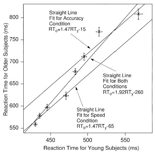
Brinley functions for correct response times (RTs) for the experiment. The points on the graph represent the same conditions for older and young subjects. Straight lines are fitted for speed and accuracy conditions separately and for the conditions combined. Error bars are 2 SEs in mean RT. The four data points in the bottom left of the figure are for the speed conditions, and the four data points in the top right of the figure are for the accuracy conditions.

Calculating the slope of the Brinley function as m = SD_o/SD_y, where SD represents the standard deviation in the mean response times across conditions (see Ratcliff et al., 2000, and Draper & Smith, 1998) and the intercept as c = mean RT_o − m mean RT_y, then for the speed conditions, RT_o = 1.52RT_y − 85 ms, and for the accuracy conditions, RT_o = 1.55RT_y − 59 ms; and for both combined, RT_o = 1.98RT_y − 283 ms. The fact that the slope varies according to whether all or part of the data are plotted illustrates one of the problems with the slowing hypothesis: It would not be expected that the amount of cognitive slowing for older subjects relative to young ones would depend on whether speed and accuracy conditions are fitted separately or combined.

The approximate equality of slopes for the speed and accuracy conditions differs from results obtained by Ratcliff et al. (2000, Experiment 2), where the slopes were different for speed and accuracy conditions, 1.46 and 2.62, respectively. That experiment also differs from the one here in that accuracy rates were approximately the same for older and young subjects, which is not the case here. These comparisons between experiments suggest that there is likely to be no simple and general pattern of effects of speed–accuracy manipulations on Brinley function slopes.

The standard error bars around the data points in Figure 3 illustrate a problem rarely discussed in the Brinley function literature: Does a straight line actually fit the data? The straight line fit to the speed conditions intersects confidence ellipses for all four data points, but the line for the accuracy conditions intersects only two out of four confidence ellipses, and the line fit to all of the data combined intersects only four out of eight. Thus, although the Brinley functions look typical of those found in the literature, a straight line does not provide a good fit for the accuracy conditions or for both conditions combined. It might be that a straight line does provide the best account of processing, and it is other factors, such as averaging, subjects truncating their long responses, and so on, that account for the deviations. Or it might be that a linear function truly is not the best account of processing, and so that is the reason for the poor fit.

It should also be mentioned that the use of Brinley functions has sometimes had a prerequisite that accuracy values be equivalent (e.g., Myerson et al., 1990) for old and young subjects. In our experiment reported here, the accuracy values were considerably lower for the older subjects than for the young subjects. If accuracy values are not equivalent, there is no common agreed method for interpreting the functions, although there have been a number of attempts to address the covariation of the two variables (e.g., Cerella, 1985; Kliegl, Mayr, & Krampe, 1994; Salthouse, 1996; G.A. Smith & Brewer, 1995). Because the diffusion model makes predictions about both accuracy and response time, it provides a theoretically based means of dealing with this problem, as illustrated below.

Results: Quantile Probability Functions

To fully test the diffusion model, it is simultaneously fit to all aspects of the data: accuracy rates, correct and error response times, and response time distributions. Plotting all of these aspects of the data separately would make their relative behaviors difficult to grasp, so the data are displayed in quantile probability functions (Figures 4 and 5).

Figure 4.

Quantile-probability functions for older subjects. The lines represent the fits of the diffusion model and the xs represent the data. The lines in order from the bottom to the top are for the .1, .3, .5, .7, and .9 quantile response times. Correct responses are to the right of the .5 response probability point, and the corresponding error responses are to the left (if the correct response probability is p, the error response probability is 1 − p).

Figure 5.

Quantile-probability functions for young subjects. The lines represent the fits of the diffusion model, and the xs represent the data. The lines in order from the bottom to the top are for the .1, .3, .5, .7, and .9 quantile response times. Correct responses are to the right of the .5 response probability point, and the corresponding error responses are to the left.

For quantile probability functions, the quantiles of the response time distributions for each experimental condition are plotted as a function of response probability. In Figures 4 and 5, the .1, .3, .5 (median), .7, and .9 quantiles are plotted for each of the four stimulus duration conditions (for older and young subjects and the speed and accuracy conditions separately). The xs are the data points and the lines are the best fitting functions from the diffusion model, which will be discussed later. The four right-hand points for each quantile represent correct responses in the four stimulus duration conditions. For the older subjects, for example, the probability of a correct response varies from about .85 (with the longest stimulus duration) to about .55 (with the shortest stimulus duration). The four left-hand points represent error responses in the four conditions, with the left-most point representing errors in the highest accuracy condition (which corresponds to the longest stimulus duration). The data for the left- and right-hand response alternatives were combined because there were no significant differences between them.

The quantile probability functions give a summary picture of the shapes of the response time distributions. With accuracy instructions, for correct responses, the response time distribution skews out as stimulus duration decreases. Across the four conditions, the .1 quantile response times stay about the same, but the .9 quantiles slow from about 1,000 ms to about 1,300 ms for the older subjects and from about 600 ms to 800 ms for the young subjects. With speed instructions, the skewing is much less apparent, from about 750 ms to 850 ms for the older subjects and from about 500 ms to 600 ms for the young subjects.

The quantile probability functions also show the relative speeds of correct and error responses. For example, with accuracy instructions, in the highest accuracy condition (the furthest right quantile points), response times for correct responses are about 900 ms at the .9 quantile and the error responses in that condition (the farthest left quantile points) are much slower, 1,400 ms at the .9 quantile.

For both older and young subjects, response time increases and accuracy decreases as stimulus duration decreases, and error response times are longer than correct response times. The changes in response times across conditions are smaller in the speed condition than the accuracy condition, and the minimum response times are shorter in the speed condition than in the accuracy condition. The overall shapes of the response time distributions are about the same across the experimental conditions. Averaged across stimulus duration conditions, the difference in accuracy for the speed versus accuracy conditions is about 2% for the older subjects and about 5% for the young subjects.

Overall, the data show that the older subjects differ from the young subjects in three main ways: First, the older subjects are slower than the young subjects in all conditions. Second, the older subjects are less accurate than the young subjects in all conditions, which can be seen in the quantile probability plots by the young subjects’ data points shifted further to the left and right relative to the older subjects’ data points, away from the .5 response probability point. Third, the older subjects show increasing response times for errors as error probability decreases, whereas the young subjects show decreasing response times, especially in the speed conditions. In sum, the results show regular patterns for the effects of difficulty (stimulus duration), speed versus accuracy instructions, and age on performance. The question for the diffusion model is what components of processing are responsible for these effects.

Results: Fitting the Diffusion Model

The diffusion model was fit to the data by minimizing a chi-square value with a general SIMPLEX minimization routine that adjusts the parameters of the model to find the parameters that give the minimum chi-square value. The data entered into the minimization routine for each experimental condition were the response times for each of the five quantiles for correct and error responses and the accuracy values. The quantile response times were fed into the diffusion model, and for each quantile, the cumulative probability of a response by that point in time was generated from the model. Subtracting the cumulative probabilities for each successive quantile from the next higher quantile gives the proportion of responses between each quantile. For the chi-square computation, these are the expected values, to be compared with the observed proportions of responses between the quantiles (multiplied by the number of observations). The observed proportions of responses for each quantile are the proportions of the distribution between successive quantiles (i.e., the proportions between 0, .1, .3, .5, .7, .9, and 1.0 are .1, .2, .2, .2, .2, and .1) multiplied by the probability correct for correct response distributions or the probability of error for error response distributions (in both cases, multiplied by the number of observations). Summing over (Observed − Expected)²/Expected for all conditions gives a single chi-square value to be minimized.

In their research on fitting the diffusion model to data, Ratcliff and Tuerlinckx (2002), found that when long or short outlier response times were added to simulated data, the chi-square method could not accurately recover the parameter values that were used to generate the data. To address this problem, short outliers (response times shorter than 300 ms for young subjects and 350 ms for older subjects) are trimmed out by examining the time at which accuracy begins to rise above chance (e.g., Swensson, 1972), and long outliers (responses longer than 2,000 ms for young subjects and 3,000 ms for older subjects) are also eliminated from the analyses. Ratcliff and Tuerlinckx showed that any remaining contaminant response times can be explicitly modeled. A parameter (p_o) is added to represent the probability of a contaminant in each condition of the experiment. Contaminants are assumed to come from a uniform distribution with maximum and minimum values corresponding to the maximum and minimum response times in the condition. For the data reported here, the value of the probability parameter, p_o, was the same across all experimental conditions (speed and accuracy and the different levels of difficulty). There might be reasonable alternative assumptions for the distribution of contaminants, but the small proportion usually estimated (less than 2% here), the ease of implementation, the fact that this adds only one parameter to the model, and the ability to recover parameter values better than methods without this assumption (Ratcliff & Tuerlinckx, 2002) all indicate that this was a reasonable approximation.

For the fits of the model presented here, five parameters were held constant across the four stimulus duration conditions and speed versus accuracy instructions: T_er, across trial variability in the nondecision component of processing (s_t), the range of the starting point of the diffusion process across trials (s_z), across trial variability in drift rate (η), and the probability of contaminant response times (p_o). Holding these five parameters constant reflects the assumption that neither speed versus accuracy instructions nor the quality of the information from the stimulus (stimulus duration) affects any of these components of the decision process.

Boundary separation was assumed to be constant across stimulus duration conditions, with one value of separation for the speed conditions and a different value for the accuracy conditions. If boundary separation were to vary with stimulus duration condition, it would mean that subjects had identified the condition, adjusted the boundary separation, and then begun extracting information from the stimulus. This sequence of events is not plausible. Also, changes in boundary separation with duration conditions would produce changes in the .1 quantile response times that are not observed in the data.

Drift rates were assumed to be constant across the speed and accuracy conditions because the quality of information from the stimulus should not change with these instructions. Drift rates were assumed to vary only with stimulus duration.

The model must account for accuracy rates, the relative speeds of correct and error responses, and the shapes of the response time distributions for correct and error responses. Specifically, with only boundary separation varying, the model must account for the small changes in accuracy and the large changes in response time between the speed and accuracy conditions. With only drift rate varying, the model must account for the changes as a function of stimulus duration in accuracy and distribution shape for both error and correct responses and for both the speed and accuracy conditions.

We fit the diffusion model to the data in two ways. First, each subject’s data were fit individually and the parameter values averaged across subjects. The means for each of the parameters are shown in Table 2 along with their standard deviations. Standard errors in the parameter values can be found by dividing the standard deviations by the square root of the number of subjects (40 young subjects or 38 older subjects). The second fits of the model were to the data averaged across all of the older subjects and all of the young subjects. These fits were used as the basis for the predictions displayed in Figures 4 and 5 (the solid lines). Note that the parameter values obtained from the group data and the average parameter values across individuals are all within 2 SEs of each other (see Table 2). Also, the parameter values are in the range of parameter values from other experiments (Ratcliff, 2002; Ratcliff & Rouder, 1998, 2000; Ratcliff et al., 1999, 2001, 2003).

Table 2.

Parameter Values and Standard Errors From Fits of the Diffusion Model

Condition	Subjects	as	aa	Ter	η	sz	v1	v2	v3	v4	po	st
Subjects	Old	0.107	0.168	0.413	0.276	0.034	0.043	0.112	0.214	0.305	0.006	0.136
M data	Old	0.103	0.162	0.407	0.231	0.010	0.039	0.094	0.183	0.266	0.000	0.143
Subjects	Young	0.084	0.122	0.343	0.239	0.053	0.140	0.317	0.427	0.491	0.007	0.112
M data	Young	0.079	0.121	0.353	0.246	0.055	0.141	0.313	0.423	0.487	0.005	0.126
SDs over subjects	Old	0.034	0.039	0.048	0.092	0.032	0.044	0.070	0.089	0.105	0.016	0.053
SDs over Subjects	Young	0.016	0.032	0.032	0.094	0.019	0.089	0.126	0.154	0.159	0.012	0.045

Note. a_s = boundary separation for speed condition; a_a = boundary separation for accuracy condition; T_er = nondecision component of response time; η = standard deviation in drift across trials; s_z = range of the distribution of starting point (z); v = drift rates; p_o = proportion of contaminants; s_t = range of the distribution of the nondecision component of processing. In the subjects condition, the model was fit to each individual subject and the parameter values averaged over the subjects’ values. The SDs were standard deviations over the parameter values for the fits for the individual subjects. In the M data condition, the model was fit to the data averaged over subjects.

In general, the fits are good. The model captures the changes in response time and accuracy as a function of stimulus duration and speed versus accuracy instructions for both correct and error responses as well as the overall differences between the older and young subjects. The only noticeable misses are in the .9 quantile response times for the older subjects with accuracy instructions; the model predicts longer response times than the data, but the misses are not severe given the high variability in long response times. The young subjects have .9 quantile response times less than 1,000 ms, and their fits do not systematically deviate from the data.

The systematic misfits in the .9 quantile response times for older subjects in the accuracy conditions might be due to the subjects calling it quits after 1 to 2 s of processing or they might be due to the boundary separation being reduced after about a second of processing (e.g., Luce, 1986, p. 375). The diffusion model predicts that some proportion of the response time distribution tails extends into 2, 3, or 4 s, given the parameters of the fits for older subjects in the accuracy conditions. If subjects truncated these long duration processes, then the .9 quantile response times would be reduced. To examine the effect of such truncation, we refit the diffusion model to the data with the assumption that all responses were terminated by 2,000 ms and response times that would have terminated after 2,000 ms were eliminated. The .1, .3, and .5 quantile response times were hardly altered, but the .7 quantile response times were decreased from the predicted values by 9 ms and the .9 quantile response times were decreased by 33 ms. The change in the .7 quantile hardly alters the quality of the fit in Figure 4, but the change in the .9 quantile reduces the location of the predicted .9 quantile function such that it does not deviate systematically from the data. Thus the model’s mispredictions can be explained if it is the case that older subjects are unwilling to wait several seconds for a very slow decision process to end.

For the young and older subjects, respectively, the chi-square goodness-of-fit values were reasonable, 84.1 and 119.1 with df = 77; the critical chi-square value is 98.5 for p = .05. For the individual fits, for young subjects, the mean value of chi-square was 100.8 (SD = 37.7) and for older subjects, the mean value of chi-square was 82.3 (SD = 25.9). The number of chi-square values significant was 21/40 for young subjects and 11/38 for older subjects. These values show the model fits most individual subject data at about a level that is borderline significant, on average about as well as the fits shown in Figures 4 and 5.

Analysis of the parameter estimates showed that the older subjects differed from the young subjects in three ways. For both groups of subjects, there is a healthy drop of about 30% in boundary separation going from accuracy to speed instructions. With both kinds of instructions, the older subjects have wider boundary separations than the young subjects by about 20%, t(76) = 3.81, p < .05, and t(76) = 5.63, p < .05, for speed and accuracy instructions, respectively. The value of T_er was larger for older subjects than young subjects by about 50 to 70 ms, t(76) = 7.57, p ≤ .05. Both of these results replicate those of Ratcliff et al. (2001). However, different from Ratcliff et al. (2001), drift rates were lower for the older subjects than the young subjects, t(76) = 6.02, 8.84, 7.43, and 6.08, p ≤ .05, for the four stimulus duration conditions, long to short, respectively: The drift rates were about one half the size for older subjects as for young subjects. This translates into differences as large as 200 ms in mean response time and 10% in accuracy, indicating that the quality of the stimulus information is much lower for the older subjects than for the young subjects. In other words, the older subjects were obtaining stimulus information from the display at about one half the rate of the young subjects.

There were no significant differences between the older and young subjects in between-trial variability in drift rate (η), starting point (s_z), or the nondecision component of response time (s_t). Also, for both groups of subjects and in all experimental conditions, the estimated probability of contaminants was less than 1%.

Figures 6 and 7 present histograms of the distributions of the parameter values from the individual subject fits for the young and older subjects. First, the distributions for T_er and drift rates are symmetrical (except perhaps for v₁, the lowest drift rate, which has a few large values for both the old and young subjects; apparently these subjects could see the stimulus letters at the 10-ms stimulus duration). Second, the distributions for boundary separation are a little right-skewed. This is probably because of scaling: Boundary separation can be increased without bound, but it cannot be decreased below zero (or more realistically, some minimum around .04 or .05). Third, the distributions of η are roughly symmetrical. Fourth, the distributions of s_z have some values near zero for the older subjects, and the distributions of variability in T_er have some values near zero for both the older and the young subjects. These near-zero values might arise from having relatively few observations in extreme error conditions for some subjects (i.e., the fitting program may estimate low values because of a lack of stability in the data). The fitting program compensates for a low value of s_t with a lower value of T_er and a larger value of boundary separation. These values of T_er and boundary separation give rise to relatively high values of correlations between boundary separation a and T_er for older subjects. If we eliminate the 8 (out of 38) subjects with the largest boundary separations, the correlations drop to −.19 and −.22. Of these 8 subjects, 6 also have the lowest values of s_t.

Figure 6.

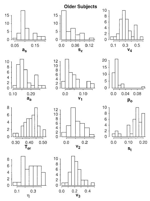
Histograms for the parameter values for older subjects for fits of the diffusion model.

Figure 7.

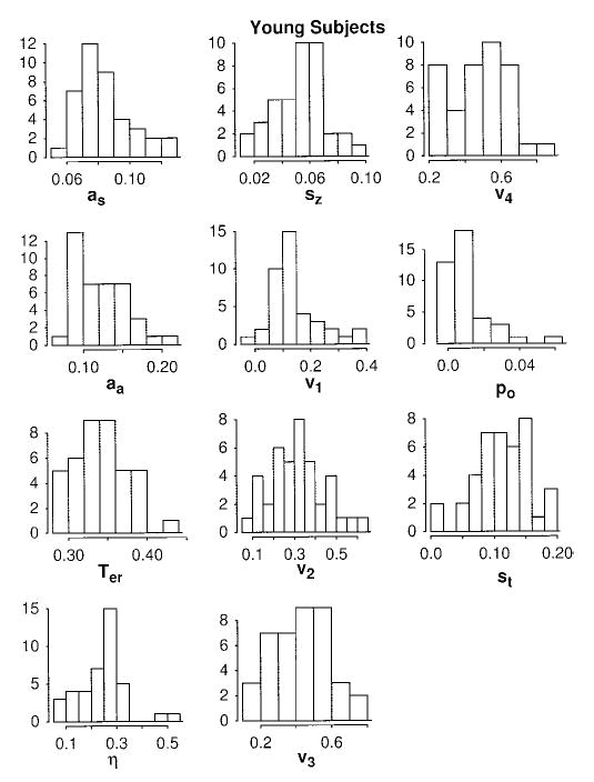
Histograms for the parameter values for young subjects for fits of the diffusion model.

The main result from Figures 6 and 7 is that there is nothing surprising about the parameter values across individuals. With the exceptions noted above, the distributions appear quite symmetric. The most straightforward interpretation of this is that each of the components of processing represented by the parameter values is selected from a roughly symmetric distribution and individuals do not deviate systematically from this pattern.

Tables 3 and 4 show correlations among subjects’ parameter values for the two groups of subjects. We point out the more important effects, those where there are high correlations for both groups of subjects. First, boundary separations for the speed and accuracy instructions are positively correlated. If a subject sets a relatively wide separation in the speed condition, they also do so in the accuracy condition. Second, drift rates are highly correlated with each other. This means that if a subject is obtaining good information at one stimulus duration relative to other subjects, then the subject is also obtaining good information at the other stimulus durations. Third, T_er is correlated with s_t, which means that if T_er is large, then s_t is also large (this is another scaling effect). Fourth, the drift rates are correlated with variability in drift. If the drift rates are high, then the variability in drift across trials is also high. This again can be seen as a scaling effect.

Table 3.

Correlations Between Parameter Values for Individual Subjects for Young Subjects

Variable	1	2	3	4	5	6	7	8	9	10	11
1. as	1.00
2. aa	.53	1.00
3. Ter	.15	.16	1.00
4. η	.37	.02	.06	1.00
5. sz	.63	.22	.16	.43	1.00
6. v1	.07	−.11	−.34	.47	−.02	1.00
7. v2	.01	−.27	−.25	.64	−.08	.79	1.00
8. v3	−.03	−.22	−.19	.63	−.14	.72	.94	1.00
9. v4	−.01	−.20	−.12	.71	−.06	.61	.91	.94	1.00
10. Po	−.29	−.08	.07	−.25	−.04	−.18	−.18	−.22	−.15	1.00
11. st	−.17	.10	.87	.08	.21	−.28	−.24	−.19	−.15	.13	1.00

Note. a_s = boundary separation for speed condition; a_a = boundary separation for accuracy condition; T_er = mean of the nondecision component of response time; η = standard deviation in drift across trials; s_z = range of the distribution of starting point (z); v = drift rates, p_o = proportion of contaminants; s_t = range of the distribution of the nondecision component of processing. A single correlation of plus or minus .31 would be significant at a .05 level.

Table 4.

Correlations Between Parameter Values for Individual Subjects for Older Subjects

Variable	1	2	3	4	5	6	7	8	9	10	11
1. as	1.00
2. aa	.63	1.00
3. Ter	−.72	−.57	1.00
4. η	.19	.09	−.22	1.00
5. sz	.24	.47	−.14	.22	1.00
6. v1	−.03	.14	−.12	.10	.22	1.00
7. v2	.26	.07	−.20	.45	.20	.51	1.00
8. v3	.11	−.02	−.15	.56	.15	.48	.81	1.00
9. v4	.09	−.03	−.09	.70	.16	.43	.77	.92	1.00
10. Po	.04	.45	−.13	.04	.32	−.14	−.15	−.23	−.09	1.00
11. st	−.54	−.39	.67	−.22	−.35	−.03	−.04	.01	.05	−.09	1.00

Note. a_s = boundary separation for speed condition; a_a = boundary separation for accuracy condition; T_er = mean of the nondecision component of response time; η = standard deviation in drift across trials; s_z = range of the distribution of starting point (z); v = drift rates; p_o = proportion of contaminants; s_t = range of the distribution of the nondecision component of processing. A single correlation of plus or minus .32 would be significant at a .05 level.

We also performed a correlational analysis on the parameter values and the experimental data for the older and young subjects combined. The aim was to see if individual differences in response time or accuracy were related to or determined by single parameters of the model. The experimental data were the correct and error response time means, the .1 quantile response times for correct responses, and accuracy, each averaged across all of the experimental conditions. The .1 quantile response times showed the same pattern of correlations as the mean response time, so it is not reported. We reduced the number of parameters presented (e.g., Table 5) first by eliminating parameters that did not correlate highly with any of the data (η, s_z, and s_t), and second by combining parameters that showed the same patterns of correlations, namely the two boundary separations and the four drift rates.

Table 5.

Correlations Between Parameter Values and Data for Individual Subjects

Parameter	1	2	3	4	5	6
1. Mean a	1.00	—
2. Ter	.05	1.00	—
3. Mean v	−.38	−.53	1.00	—
4. Accuracy	−.43	−.63	.86	1.00	—
5. Mean RT	.77	.58	−.77	−.77	1.00	—
6. Mean error RT	.90	.40	−.61	−.61	.94	1.00

Note. a = average boundary separation for speed and accuracy conditions; T_er = nondecision component of response time (RT); v = mean of the four drift rates for the four stimulus duration conditions. A single correlation of .22 would be significant at a .05 level.

Table 5 shows the correlations, and Figure 8 displays the scatter plots. Drift rate correlates strongly positively with accuracy and strongly negatively with both correct and error response times. This means that the better the information extracted from the stimulus, the higher is accuracy and the shorter are correct and error response times. Boundary separation is strongly positively correlated with mean correct and error response times. This is because the more widely subjects set boundaries, the slower are responses. There is a weaker correlation of boundary separation with accuracy, suggesting that subjects with poorer extraction of evidence attempted to compensate by setting more conservative boundary separations. But examination of the scatter plot in Figure 8 suggests that this is not a strong relationship. T_er is correlated moderately negatively with accuracy and positively with response time for both correct and error responses. This indicates that if the nondecision components of response time are long, then the extraction of stimulus information is somewhat poorer than if the nondecision components are short. Finally, accuracy and response times are highly negatively correlated because subjects are generally fast and accurate or slow and inaccurate.

Figure 8.

Scatter plots of parameters of the diffusion model and data for individual subjects. The parameters are the average of the boundary separation parameters for speed and accuracy, the value of the nondecision component of response time (RT), and the average of the four drift rates. The data are values of accuracy, mean correct RT, and mean error RT. These were averaged over experimental conditions (stimulus duration) and over speed and accuracy conditions.

The correlations between the parameter values and the data indicate that it is not possible, in the diffusion model framework, to interpret the effects of aging as showing a decrement in a single parameter or a single common decrement in several parameters. Drift rates measure the quality of information extracted from the stimuli, and the better the quality, the more accurate and faster the responses. Boundary separation measures speed–accuracy criterion setting, and subjects are able to improve accuracy by a few percentages at the expense of several hundred milliseconds in response time. Average drift rate does not correlate with boundary separation, as can be seen in Tables 3, 4, and 5, which indicates that a single factor cannot be extracted from drift rates and boundary separations.

In the diffusion model, the equality of the slopes of the Brinley functions for the speed and accuracy conditions is explained by two factors balancing each other. The drift rates (and accuracy values) for the older subjects are lower than for the young subjects, and there are smaller differences in drift rates among conditions for the older subjects relative to the young subjects. Also, boundary separations are larger for older subjects than young subjects. This combination (both lower values of, and smaller differences in, drift rates and wider boundary separations) leads to equal slopes in Brinley functions for the speed and accuracy conditions.

General Discussion

The experiment reported in this article shows, unsurprisingly, that older subjects are slower and less accurate than young subjects in a letter identification task with masked stimuli. With speed instructions, median response times for correct responses for young subjects were between 380 and 410 ms and accuracy values were between .65 and .90, whereas for older subjects the values were between 520 and 570 ms and .55 and .80, respectively. With accuracy instructions, correct median response times for young subjects were between 460 and 520 ms and accuracy values were between .69 and .94, while for older subjects they were between 620 and 720 ms and .56 and .84, respectively.

The deficits in performance between old and young are large both in accuracy and response time. In earlier work, with a signal detection task, Ratcliff et al. (2001) found a deficit only in response time; accuracy levels were about the same for old and young. In the signal detection task, subjects were asked to judge whether the number of asterisks presented in a 10 × 10 array on a computer monitor was large or small, and the array remained on the screen until a response key was pressed. Thus there were no limiting perceptual or memory demands on the subjects, and so it might be expected that the older subjects would not show a deficit in accuracy. But in the experiment in this article, the short presentation time for the letter stimuli, coupled with an immediate mask, restricts perceptual processing. The result is that accuracy falls for the older subjects relative to the young ones, indicating a decrement in performance that is more than just a decrement in processing speed. Whether this decrement generalizes to all perceptually limited tasks is an open question.

Brinley function analyses of the data showed that when response time means for correct responses are plotted for the speed and accuracy conditions separately, the slopes of the functions are both about 1.54, but when the speed and accuracy conditions are combined, the slope is 1.98. The often noted Brinley function regularity, that slope values should remain relatively constant, was not obtained; the slope values were different when conditions were separated than when they were combined. The regularity also did not appear with the signal detection task used by Ratcliff et al. (2001), for which different slope values were obtained for the speed and accuracy conditions (1.4 and 2.6, respectively).

The diffusion model fit all aspects of data reported in this experiment, including accuracy rates and distributions of response times for both correct and error responses. The analysis of the components of processing provided by the diffusion model is consistent in three respects with the account that was provided for the signal detection experiment (Ratcliff et al., 2001). First, the parameter estimates produced by the model indicate that older subjects are more conservative than young subjects in that they set response boundaries wider apart, in essence requiring more information before reaching a decision. Second, the nondecision components of response time, summarized by T_er, are 50 to 60 ms longer for older subjects than young subjects. Third, the parameters representing variability in drift and starting point are similar for older and young subjects. The important difference between the results obtained here and the results obtained by Ratcliff et al. (2001) lies in drift rates, which reflect the quality of the information entering the decision process from the stimuli. For the signal detection task used by Ratcliff et al. (2001), the drift rates were the same for older and young subjects. But here, drift rates are lower, about one half the size, for older subjects than for young subjects. In other words, for the quickly flashed letter stimuli, the older subjects extracted about one half of the information per unit time compared with the young subjects.

The lower drift rates for the older subjects suggest an explanation for why older subjects set more conservative decision criteria than young subjects even in experiments for which there are no perceptual or memory limitations, experiments such as the signal detection experiment where drift rates were the same for older and young subjects. If we assume that the decision criteria, that is the boundary positions of the diffusion process, are set at about the same values across tasks, then it may be that older subjects set conservative criteria in all tasks in order to compensate for their difficulties in those tasks that have perceptual or memory limitations.

There are a number of other sequential sampling models of the same general class as the diffusion model presented here. Ratcliff and Smith (in press) examined them in detail and concluded that the diffusion model provides the best overall account of data. Another candidate model is the Ornstein–Uhlenbeck model (see Smith, 1995). It is the same as the diffusion model except that drift rate is assumed to decay as a function of position away from the starting point. When decay is small or moderate, this model mimics the diffusion model (Ratcliff & Smith, in press) and so, as long as decay was not large, it could fit the data presented here. Another candidate model is an accumulator model with criteria that are exponentially distributed across trials (see Ratcliff & Smith for the most successful versions of this model). The accumulator model assumes that evidence from a stimulus is normally distributed, and that discrete, repeated samples are taken from this distribution. If the evidence is positive, it is added to one counter, and if it is negative, it is added to a second counter. Evidence is accumulated until one of the counters reaches a criterion. If the criteria are variable and exponentially distributed across trials, the model does a good job of fitting data except that it is unable to predict error response times shorter than correct response times, a pattern that occurs in many tasks. It would be able to fit the data from the experiment presented here because errors are slower than correct responses. Also, the model fits the data from Experiment 2, Ratcliff et al. (2001), which are similar to the data presented here. For this experiment, the conclusions from the accumulator model would be similar to those from the diffusion model. Changes in decision criteria lead to large changes in response time, but relatively small changes in accuracy. Thus, fits of the model would produce lower rates of accumulation for older subjects relative to young subjects in the accumulator model just as in the diffusion model.

The diffusion model captures the deficit in accuracy for older subjects while simultaneously capturing their longer response times. The interpretation provided by the model is that older subjects have a lower rate of extraction of information from masked letter stimuli than young subjects, a finding that is consistent with earlier research on age deficits in visual perception (Fozard, 1990; Spear, 1993). The earlier literature is based on accuracy measures, so the diffusion model provides a means of reconciling the findings of that literature with the results of tasks that measure response time. On the basis of earlier findings, we would expect that the age deficit observed in the rate of extraction of information in letter identification is not the result of a general deficit but a task-specific deficit for high spatial contrast stimuli. The crucial next step will be to test this expectation, using a variety of kinds of perceptual stimuli.

References

- Allen PA, Ashcraft MH, Weber TA. On mental multiplication and age. Psychology and Aging. 1992;7:536–545. doi: 10.1037//0882-7974.7.4.536. [DOI] [PubMed] [Google Scholar]
- Allen PA, Madden DJ, Weber TA, Groth KE. Influence of age and processing stage on visual word recognition. Psychology and Aging. 1993;8:274–282. doi: 10.1037//0882-7974.8.2.274. [DOI] [PubMed] [Google Scholar]
- Birren, J. E. (1965). Age-changes in speed of behavior: Its central nature and physiological correlates. In A. T. Welford & J. E. Birren (Eds.), Behavior, aging, and the nervous system (pp. 191–216). Springfield, IL: Charles C Thomas.
- Brinley, J. F. (1965). Cognitive sets, speed and accuracy of performance in the elderly. In A. T. Welford & J. E. Birren (Eds.), Behavior, aging and the nervous system (pp. 114–149). Springfield, IL: Thomas.
- Busemeyer JR, Townsend JT. Decision field theory: A dynamic–cognitive approach to decision making in an uncertain environment. Psychological Review. 1993;100:432–459. doi: 10.1037/0033-295x.100.3.432. [DOI] [PubMed] [Google Scholar]
- Cerella J. Information processing rates in the elderly. Psychological Bulletin. 1985;98:67–83. [PubMed] [Google Scholar]
- Cerella, J. (1990). Aging and information-processing rate. In J. E. Birren & K. W. Schaie (Eds.), Handbook of the psychology of aging (3rd ed., pp. 201–221). San Diego, CA: Academic Press.
- Cerella J. Age effects may be global, not local: Comment on Fisk and Rogers (1991) Journal of Experimental Psychology: General. 1991;120:215–223. doi: 10.1037/0096-3445.120.2.215. [DOI] [PubMed] [Google Scholar]
- Cerella J. Generalized slowing in Brinley plots. Journal of Gerontology: Psychological Sciences. 1994;49:65–71. doi: 10.1093/geronj/49.2.p65. [DOI] [PubMed] [Google Scholar]
- Coyne AC, Burger MC, Berry JM, Botwinick J. Adult age, information processing, and partial report performance. Journal of Genetic Psychology. 1987;148:219–224. doi: 10.1080/00221325.1987.9914551. [DOI] [PubMed] [Google Scholar]
- Cramer G, Kietzman ML, Van Laer J. Dichoptic backward masking of letters, words, and trigrams in old and young subjects. Experimental Aging Research. 1982;8:103–108. doi: 10.1080/03610738208258405. [DOI] [PubMed] [Google Scholar]
- Di Lollo V, Arnett JL, Kruk RV. Age-related changes in rate of visual information processing. Journal of Experimental Psychology: Human Perception and Performance. 1982;8:225–237. doi: 10.1037/0096-1523.8.2.225. [DOI] [PubMed] [Google Scholar]
- Draper, N. R., & Smith, H. (1998). Applied regression analysis. New York: Wiley.
- Faust ME, Balota DA, Spieler DH, Ferraro FR. Individual differences in information-processing rate and amount: Implications for group differences in response latency. Psychological Bulletin. 1999;125:777–799. doi: 10.1037/0033-2909.125.6.777. [DOI] [PubMed] [Google Scholar]
- Fisher DL, Glaser RA. Molar and latent models of cognitive slowing: Implications for aging, dementia, depression, development, and intelligence. Psychonomic Bulletin & Review. 1996;3:458–480. doi: 10.3758/BF03214549. [DOI] [PubMed] [Google Scholar]
- Fisk AD, Fisher DL. Brinley plots and theories of aging: The explicit, muddled, and implicit debates. Journal of Gerontology: Psychological Sciences. 1994;49:81–89. doi: 10.1093/geronj/49.2.p81. [DOI] [PubMed] [Google Scholar]
- Fisk JE, Warr P. Age and working memory: The role of perceptual speed, the central executive, and the phonological loop. Psychology and Aging. 1996;11:316–323. doi: 10.1037//0882-7974.11.2.316. [DOI] [PubMed] [Google Scholar]
- Folstein MF, Folstein SE, McHugh PR. Mini-mental state: A practical method for grading the cognitive state of patients for the clinician. Journal of Psychiatric Research. 1975;12:189–198. doi: 10.1016/0022-3956(75)90026-6. [DOI] [PubMed] [Google Scholar]
- Fozard, J. L. (1990). Vision and hearing in aging. In J. E. Birren & K. W. Schaie (Eds.), Handbook of the psychology of aging (pp. 150–170). San Diego, CA: Academic Press.
- Hale S, Jansen J. Global processing-time coefficients characterize individual and group differences in cognitive speed. Psychological Science. 1994;5:384–389. [Google Scholar]
- Hale S, Myerson J, Wagstaff D. General slowing of nonverbal information processing: Evidence for a power law. Journal of Gerontology. 1987;42:131–136. doi: 10.1093/geronj/42.2.131. [DOI] [PubMed] [Google Scholar]
- Hartley, A. A. (1992). Attention. In F. Craik & T. Salthouse (Eds.), The handbook of aging and cognition (pp. 3–49). Hillsdale, NJ: Erlbaum.
- Hertzog, C. (1992). Aging, information processing, and intelligence. In K. W. Schaie (Ed.), Annual review of gerontology and geriatrics (Vol. 11, pp. 55–79). New York: Springer.
- Hertzog C, Vernon MC, Rympa B. Age differences in mental rotation task performance: The influence of speed/accuracy tradeoffs. Journal of Gerontology. 1993;48:150–156. doi: 10.1093/geronj/48.3.p150. [DOI] [PubMed] [Google Scholar]
- Hertzog CK, Williams MV, Walsh DA. The effect of practice on age differences in central perceptual processing. Journal of Gerontology. 1976;31:428–433. doi: 10.1093/geronj/31.4.428. [DOI] [PubMed] [Google Scholar]
- Kaufman, A. (1990). Assessing adolescent and adult intelligence. Boston: Allyn & Bacon.
- Kliegl R, Mayr U, Krampe RT. Time–accuracy functions for determining process and person differences: An application to cognitive aging. Cognitive Psychology. 1994;26:134–164. doi: 10.1006/cogp.1994.1005. [DOI] [PubMed] [Google Scholar]
- Kline DW, Nestor S. Persistence of complementary afterimages as a function of adult age and exposure duration. Experimental Aging Research. 1977;3:191–201. doi: 10.1080/03610737708257102. [DOI] [PubMed] [Google Scholar]
- Kline DW, Orme-Rogers C. Examination of stimulus persistence as the basis for superior visual identification performance among older adults. Journal of Gerontology. 1978;33:76–81. doi: 10.1093/geronj/33.1.76. [DOI] [PubMed] [Google Scholar]
- Lima SD, Hale S, Myerson J. How general is general slowing? Evidence from the lexical domain. Psychology and Aging. 1991;6:416–425. doi: 10.1037//0882-7974.6.3.416. [DOI] [PubMed] [Google Scholar]
- Luce, R. D. (1986). Response times. New York: Oxford University Press.
- Madden DJ. Visual word identification and age-related slowing. Cognitive Development. 1989;4:1–29. [Google Scholar]
- Madden DJ, Pierce TW, Allen PA. Adult age differences in attentional allocation during memory search. Psychology and Aging. 1992;7:594–601. doi: 10.1037//0882-7974.7.4.594. [DOI] [PubMed] [Google Scholar]
- Maylor EA, Rabbitt PMA. Applying Brinley plots to individuals: Effects of aging on performance distributions in two speeded tasks. Psychology and Aging. 1994;9:224–230. doi: 10.1037//0882-7974.9.2.224. [DOI] [PubMed] [Google Scholar]
- McDowd JM, Craik FIM. Effects of aging and task difficulty on divided attention performance. Journal of Experimental Psychology: Human Perception and Performance. 1988;14:267–280. doi: 10.1037/0096-1523.14.2.267. [DOI] [PubMed] [Google Scholar]
- Myerson J, Adams DR, Hale S, Jenkins L. Analysis of group differences in processing speed: Brinley plots, Q–Q plots, and other conspiracies. Psychonomic Bulletin and Review. 2003;10:224–237. doi: 10.3758/bf03196489. [DOI] [PubMed] [Google Scholar]
- Myerson J, Ferraro FR, Hale S, Lima SD. General slowing in semantic priming and word recognition. Psychology and Aging. 1992;7:257–270. doi: 10.1037//0882-7974.7.2.257. [DOI] [PubMed] [Google Scholar]
- Myerson, J., & Hale, S. (1993). General slowing and age invariance in cognitive processing: The other side of the coin. In J. Cerella et al. (Eds.), Adult information processing: Limits on loss (pp. 115–141). San Diego, CA: Academic Press.
- Myerson J, Hale S, Wagstaff D, Poon LW, Smith GA. The information–loss model: A mathematical theory of age-related cognitive slowing. Psychological Review. 1990;97:475–487. doi: 10.1037/0033-295x.97.4.475. [DOI] [PubMed] [Google Scholar]
- Myerson J, Wagstaff D, Hale S. Brinley plots, explained variance, and the analysis of age differences in response latencies. Journal of Gerontology: Psychological Sciences. 1994;49:72–80. doi: 10.1093/geronj/49.2.p72. [DOI] [PubMed] [Google Scholar]
- Nebes RD, Madden DJ. Different patterns of cognitive slowing produced by Alzheimer’s disease and normal aging. Psychology and Aging. 1988;3:102–104. doi: 10.1037//0882-7974.3.1.102. [DOI] [PubMed] [Google Scholar]
- Perfect TJ. What can Brinley plots tell us about cognitive aging? Journal of Gerontology: Psychological Sciences. 1994;49:60–64. doi: 10.1093/geronj/49.2.p60. [DOI] [PubMed] [Google Scholar]
- Radloff LS. The CES–D Scale: A self-report depression scale for research in the general population. Applied Psychological Measurement. 1977;1:385–401. [Google Scholar]
- Ratcliff R. A theory of memory retrieval. Psychological Review. 1978;85:59–108. [Google Scholar]
- Ratcliff R. A theory of order relations in perceptual matching. Psychological Review. 1981;88:552–572. [Google Scholar]
- Ratcliff R. Theoretical interpretations of speed and accuracy of positive and negative responses. Psychological Review. 1985;92:212–225. [PubMed] [Google Scholar]
- Ratcliff R. Continuous versus discrete information processing: Modeling the accumulation of partial information. Psychological Review. 1988;95:238–255. doi: 10.1037/0033-295x.95.2.238. [DOI] [PubMed] [Google Scholar]
- Ratcliff R. A diffusion model account of reaction time and accuracy in a two choice brightness discrimination task: Fitting real data and failing to fit fake but plausible data. Psychonomic Bulletin and Review. 2002;9:278–291. doi: 10.3758/bf03196283. [DOI] [PubMed] [Google Scholar]
- Ratcliff, R., Gomez, P., & McKoon, G. (in press). Diffusion model account of lexical decision. Psychological Review. [DOI] [PMC free article] [PubMed]
- Ratcliff R, Rouder JF. Modeling response times for two-choice decisions. Psychological Science. 1998;9:347–356. [Google Scholar]
- Ratcliff R, Rouder JF. A diffusion model account of masking in two-choice letter identification. Journal of Experimental Psychology: Human Perception and Performance. 2000;26:127–140. doi: 10.1037//0096-1523.26.1.127. [DOI] [PubMed] [Google Scholar]
- Ratcliff, R. & Smith, P. L. (in press) A comparison of sequential sampling models for two-choice reaction time. Psychological Review. [DOI] [PMC free article] [PubMed]
- Ratcliff R, Spieler D, McKoon G. Explicitly modeling the effects of aging on response time. Psychonomic Bulletin and Review. 2000;7:1–25. doi: 10.3758/bf03210723. [DOI] [PubMed] [Google Scholar]
- Ratcliff, R., Spieler, D., & McKoon, G. (2003). Analysis of group differences in processing speed: Where are the models of processing? Manuscript submitted for publication. [DOI] [PMC free article] [PubMed]
- Ratcliff R, Thapar A, McKoon G. The effects of aging on reaction time in a signal detection task. Psychology and Aging. 2001;16:323–341. [PubMed] [Google Scholar]
- Ratcliff R, Tuerlinckx F. Estimation of the parameters of the diffusion model: Approaches to dealing with contaminant reaction times and parameter variability. Psychonomic Bulletin and Review. 2002;9:438–481. doi: 10.3758/bf03196302. [DOI] [PMC free article] [PubMed] [Google Scholar]
- Ratcliff R, Van Zandt T, McKoon G. Connectionist and diffusion models of reaction time. Psychological Review, . 1999;106:261–300. doi: 10.1037/0033-295x.106.2.261. [DOI] [PubMed] [Google Scholar]
- Roe RM, Busemeyer JR, Townsend JT. Multialternative decision field theory: A dynamic connectionist model of decision making. Psychological Review. 2001;108:370–392. doi: 10.1037/0033-295x.108.2.370. [DOI] [PubMed] [Google Scholar]
- Salthouse, T. A. (1985). A theory of cognitive aging. Amsterdam: North-Holland.
- Salthouse, T. A. (1991). Theoretical perspectives on cognitive aging. Hillsdale, NJ: Erlbaum.
- Salthouse TA. The processing-speed theory of adult age differences in cognition. Psychological Review. 1996;103:403–428. doi: 10.1037/0033-295x.103.3.403. [DOI] [PubMed] [Google Scholar]
- Salthouse TA, Kausler DH, Saults JS. Utilization of path-analytic procedures to investigate the role of processing resources in cognitive aging. Psychology and Aging. 1988;3:158–166. doi: 10.1037//0882-7974.3.2.158. [DOI] [PubMed] [Google Scholar]
- Salthouse TA, Somberg BL. Isolating the age deficit in speeded performance. Journal of Gerontology. 1982;37:59–63. doi: 10.1093/geronj/37.1.59. [DOI] [PubMed] [Google Scholar]
- Schlapfer TE, Groner M, Lavoyer E, Fisch HU. Visual masking: A reliable measure for the assessment of cognitive dysfunction in the elderly? Journal of Gerontology. 1991;46:157–161. doi: 10.1093/geronj/46.4.p157. [DOI] [PubMed] [Google Scholar]
- Sliwinski MJ, Hall CB. Task-dependent cognitive slowing in the elderly: A meta-analysis using hierarchical linear models with random coefficients. Psychology and Aging. 1998;13:164–175. doi: 10.1037//0882-7974.13.1.164. [DOI] [PubMed] [Google Scholar]
- Smith GA, Brewer N. Slowness and age: Speed–accuracy mechanisms. Psychology and Aging. 1995;10:238–247. doi: 10.1037//0882-7974.10.2.238. [DOI] [PubMed] [Google Scholar]
- Smith GA, Poon LW, Hale S, Myerson J. A regular relationship between old and young adults’ latencies on their best, average and worst trials. Australian Journal of Psychology. 1988;40:195–210. [Google Scholar]
- Smith PL. Psychophysically principled models of visual simple reaction time. Psychological Review. 1995;102:567–591. [Google Scholar]
- Spear PD. Neural bases of visual deficits during aging. Vision Research. 1993;33:2589–2609. doi: 10.1016/0042-6989(93)90218-l. [DOI] [PubMed] [Google Scholar]
- Spieler DH, Balota DA, Faust ME. Stroop performance in healthy younger and older adults and in individuals with dementia of the Alzheimer’s type. Journal of Experimental Psychology: Human Perception and Performance. 1996;22:461–479. doi: 10.1037//0096-1523.22.2.461. [DOI] [PubMed] [Google Scholar]
- Swensson RG. The elusive tradeoff: Speed versus accuracy in visual discrimination tasks. Perception and Psychophysics. 1972;12:16–32. [Google Scholar]
- Till RE, Franklin LD. On the locus of age differences in visual information processing. Journal of Gerontology. 1981;36:200–210. doi: 10.1093/geronj/36.2.200. [DOI] [PubMed] [Google Scholar]
- Walsh DA. Age differences in central perceptual processing: A dichoptic backward masking investigation. Journal of Gerontology. 1976;31:178–185. doi: 10.1093/geronj/31.2.178. [DOI] [PubMed] [Google Scholar]
- Walsh, D. A., & Prasse, M. J. (1980). Iconic memory and attentional processes in the aged. In L. W. Poon, J. Fozard, L. S. Cermak, D. Arenberg, & L. W. Thompson (Eds.), New directions in memory and aging: Proceedings of the George Talland Memorial Conference (pp. 153–180). Hillsdale, NJ: Erlbaum.
- Walsh DA, Thompson LW. Age differences in visual sensory memory. Journal of Gerontology. 1978;33:383–387. doi: 10.1093/geronj/33.3.383. [DOI] [PubMed] [Google Scholar]
- Walsh DA, Till RE, Williams MV. Age differences in peripheral perceptual processing: A monoptic backward masking investigation. Journal of Experimental Psychology: Human Perception and Performance. 1978;4:232–243. doi: 10.1037//0096-1523.4.2.232. [DOI] [PubMed] [Google Scholar]
- Walsh DA, Williams MV, Hertzog CK. Age-related differences in two stages of central perceptual processes: The effects of short duration targets and criterion differences. Journal of Gerontology. 1979;34:234–241. doi: 10.1093/geronj/34.2.234. [DOI] [PubMed] [Google Scholar]
- Wechsler, D. (1981). Wechsler Adult Intelligence Scale–Revised. San Antonio, TX: Psychological Corporation.