A diffusion model analysis of the effects of aging on brightness discrimination

Abstract

The effects of aging on decision time were examined in a brightness discrimination experiment with young and older subjects (ages, 60–75 years). Results showed that older subjects were slightly slower than young subjects but just as accurate. Ratcliff’s (1978) diffusion model was fit to the data, and it provided a good account of response times, their distributions, and response accuracy. There was a 50-msec slowing of the nondecision components of response time for older subjects relative to young subjects, but response criteria settings and rates of accumulation of evidence from stimuli were roughly equal for the two groups. These results are contrasted with those obtained from letter discrimination and signal-detection-like tasks.

Overall slowing of response time (RT) is a hallmark characteristic of aging. Fisher and Glaser (1996), Ratcliff, Spieler, and McKoon (2000), Ratcliff, Thapar, and McKoon (2001), and Thapar, Ratcliff, and McKoon (in press) have recently argued that this slowing can be best understood through models that allow the various components of cognitive processes to be individually examined. Models can be useful not only in revealing which tasks suffer decrements with age, but also in identifying the components of the cognitive processes that are responsible for the observed decrements in performance.

Ratcliff et al. (2001) applied the diffusion model (Ratcliff, 1978, 1981, 1985, 1988, 2002; Ratcliff & Rouder, 1998; Ratcliff & Rouder, 2000; Ratcliff, Van Zandt, & McKoon, 1999) for simple two-choice decisions to data from a signal detection task for college-age subjects and for older subjects (ages, 60–75 years). In the diffusion model, a decision is made when information accumulated over time from a stimulus reaches one or the other of two response criteria (representing the two-choices available to the subject). Increases in mean RT can come about from changes in the response criteria, changes in the amount of information available per unit time from the stimulus, and/or changes in components of responding outside the decision process (nondecision components—e.g., stimulus encoding, response execution). Which possibility is responsible for mean RT increases in any given set of data is determined by fitting the model to correct and error RT distributions and accuracy rates. Fitting all of these dependent variables simultaneously makes the model highly constrained (see Ratcliff, 2002).

For the signal detection task they investigated, Ratcliff et al. (2001) found the usual slowing of RTs for older subjects relative to young subjects, coupled with approximately equal accuracy rates for the two groups. The diffusion model explained the longer RTs of the older subjects as a combination of a 50-msec increase in nondecision components of processing and more conservative response criteria. The rate of accumulation of information over time was the same for the older subjects as for the young. Thapar et al. (in press) also found the usual slowing of RTs for older subjects with a masked-presentation letter discrimination task, and their older subjects were less accurate than the young. The diffusion model showed the same effects as those with Ratcliff et al.’s (2001) signal detection task—a 50-msec slowing of nondecision components of RT and more conservative response criteria—but older subjects had a rate of accumulation of information that was half that of the young subjects.

In this article, we present data for young and older subjects from a two-choice, masked-brightness discrimination task and show how age-related differences in performance in this task contrast with the age-related differences in letter discrimination found by Thapar et al. (in press). We also show how the diffusion model explains this contrast and discuss how the model allows more insightful interpretations of aging effects than do earlier analyses—in particular, Brinley plot analyses (Brinley, 1965). The appropriateness of Brinley analyses has been challenged recently on a variety of fronts (see Fisher & Glaser, 1996; Ratcliff et al., 2000), and for the data presented here, we argue that the best interpretation of the effects of aging on RT comes not from Brinley plot analyses, but from the kind of comprehensive theoretical accounts that can be provided by models like the diffusion model.

One significant property of the diffusion model is that it provides an explanation of the full set of dependent variables in two-choice tasks—that is, both RT and accuracy data. In accommodating accuracy data as well as RT data, the model allows theoretical linkage between paradigms that use RT measures and those that use accuracy measures, such as threshold detection tasks. For example, if older subjects show a decrement in threshold detection, relative to young subjects, then in a two-choice version of the same task, they should show a decrement in the rate of accumulation of information from the stimulus, with the size of the decrement predictable from the threshold detection data.

Without a model that relates RT and accuracy data, the results from Ratcliff et al.’s (2001) signal detection experiments and Thapar et al.’s (in press) letter discrimination experiments would present a puzzle. For example, consider the generalized slowing hypothesis, a prominent hypothesis that has been widely accepted and attributes age-related RT differences to a slowing with age in the speed of all cognitive processes or in the speed of a general mechanism that contributes to many cognitive processes (Cerella, 1985, 1990, 1991, 1994; Fisk & Warr, 1996; Myerson, Hale, Wagstaff, Poon, & Smith, 1990; Salthouse, 1985, 1996; Salthouse, Kausler, & Saults, 1988). From the point of view of this hypothesis, the fact that the increase in mean RT for old subjects relative to young subjects is about the same size in both Ratcliff et al.’s (2001) and Thapar et al.’s experiments would indicate that cognitive processes are affected similarly by age in the two tasks. But unlike the diffusion model, the hypothesis could not explain why older and young subjects are about equally accurate in the signal detection task, but not in the letter discrimination task.

The diffusion model’s ability to integrate RT and accuracy data into a single theoretical account is highlighted in the experiment presented in this article. From Thapar et al.’s (in press) results, we know that older subjects are slowed in two-choice, masked-letter discrimination. This finding is consistent with findings in letter threshold identification tasks that show that letter identification accuracy decreases with age (Coyne, 1981; Fozard, 1990; Spear, 1993). Decreasing accuracy in letter identification can be attributed to the declining contrast sensitivity for high spatial frequencies that has been found for older subjects in experiments using sine-wave gratings (Owsley, Sekuler, & Siemsen, 1983). The diffusion model ties all of these findings to a decrease, for older subjects, in the rate of accumulation of information from high spatial frequency stimuli.

For low spatial frequency stimuli, it appears that there is little effect of age on the accuracy of threshold identification performance (Elliott, Whitaker, & MacVeigh, 1990; Owsley et al., 1983).

If this is true, the diffusion model’s account of performance with high spatial frequency stimuli can be tested. The prediction is that with low spatial frequency stimuli, the rates of accumulation of information in a two-choice task should be the same for older and young subjects. Older subjects should differ from young subjects only in other components of performance, such as nondecisional processes or response criterion settings. To implement this test of the diffusion model, we used two-choice masked-brightness discrimination.

The stimuli in the experiment were patches of black and white pixels. The subjects were asked to decide, for each patch, whether it was dark or bright (see Ratcliff, 2002). Brightness was implemented as the proportion of black to white pixels in the patch. The brightness and duration of the stimuli were manipulated to vary response accuracy from near floor to near ceiling. Although the patches have high spatial frequency information in them, the dark versus bright decision must be made on the basis of global brightness (the information that would be obtained by defocusing the eyes and judging a blurred patch). We expected that older subjects’ RTs would be longer than young subjects’ and that the increase would come from the nondecisional components of processing and, perhaps, response criteria settings. But because the required discrimination is based on low spatial frequency information, there should be no decrement in the rate of accumulation of information for the older subjects. Furthermore, if there is no decrement in the rate of accumulation of information, then (as will be explained below) there should be a difference in performance between older and young subjects in RTs, but not in accuracy.

THE DIFFUSION MODEL

The diffusion model is designed to apply only to two-choice decisions that are relatively fast and composed of a single-stage decision process (as opposed to the multiple-stage decision processes that might be involved in, e.g., reasoning or problem-solving tasks). As a rule of thumb, the model would not be applied to experiments in which mean RTs are much longer than about 1–1.5 sec. Other models in the same class as the diffusion model have been applied to decision making (Busemeyer & Townsend, 1993; Roe, Busemeyer, & Townsend, 2001) and simple RT (Smith, 1995).

The diffusion model assumes that decisions are made by a noisy process that accumulates information over time from a starting point toward one of two response criteria or boundaries, as in Figure 1, where the starting point is labeled z and the boundaries are labeled a and 0. When one of the boundaries is reached, a response is initiated. The rate of accumulation of information is called the drift rate (v), and it is determined by the quality of the information extracted from the stimulus. For example, if a “bright” stimulus was displayed for a long time prior to masking, information quality would be good, and the mean value of the drift rate toward the bright boundary would be large. Within each trial, there is noise (variability) in the process of accumulating information, so that processes with the same mean drift rate do not always terminate at the same time (producing RT distributions) and do not always terminate at the same boundary (producing errors). This source of variability is called within-trial variability. Panel A in Figure 1 shows three processes, all with the same mean drift rate toward the top boundary (shown by the arrow labeled Drift Rate). One terminates quickly at the correct boundary, another terminates more slowly, and the third terminates at the incorrect boundary.

Figure 1.

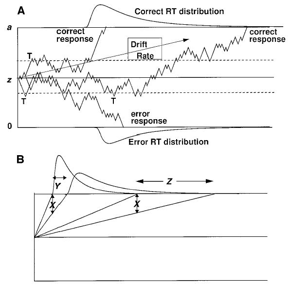
An illustration of the diffusion model. Panel A shows three sample paths and two boundary separations (the solid and the dotted lines). The points marked T represent the terminating points when the boundary positions are at the dotted lines. Panel B represents how distribution shape changes when drift rate changes by an amount X. The fastest responses slow by Y, and the slowest responses slow by Z, leading to a small shift in the leading edge of the distribution and a larger change in the tail, leading to increased skew.

In the experiment presented in this article, the subjects were instructed to respond as quickly as possible in some blocks of trials and to respond as accurately as possible in other blocks. Speed–accuracy tradeoffs are modeled by altering the boundaries of the decision process: Wider boundaries require more information before a decision can be made, and this leads to more accurate and slower responses. The dashed lines in panel A of Figure 1 show narrow boundaries. With these boundaries, the processes terminate at the points labeled T, one with a correct response and the other two with error responses.

Empirical RT distributions are positively skewed. The diffusion model naturally predicts this shape by simple geometry, as is shown in panel B of Figure 1. Moving from left to right in the figure, equal size decreases in the rate of approach to the boundary (the X values, shown by the arrows) for the fastest processes lead to increases in response time smaller than those for the slowest processes (shown by the Y and Z values, respectively).

Accounting for differences in RT between correct and error responses has long been a problem (see Luce, 1986), but in the diffusion model, the relative speeds of correct and error responses can be explained by assuming variability in components of processing across trials. Variability in drift rate across trials leads to slow error responses, and variability in starting point leads to fast error responses (see Ratcliff & Rouder, 1998; Ratcliff et al., 1999).

Besides the decision process, there are nondecision components of processing, such as encoding and response execution. These are combined in the diffusion model into one parameter, T_er (which is not shown in Figure 1). Like drift rate and starting point, T_er has variability across trials (see Ratcliff, Gomez, & McKoon, in press; Ratcliff & Tuerlinckx, 2002). Because the standard deviation in the distribution of T_er is typically less than one quarter the standard deviation in the decision process, the combination of the two (their convolution) alters neither the shape of the RT distribution (see Ratcliff & Tuerlinckx, 2002, Figure 11) nor the standard deviation for the distribution that is predicted from the decision process. For example, if the standard deviation in T_er is 25 msec and the standard deviation in the decision process is 100 msec, the combination (square root of the sum of squares) is 103 msec. Variability in T_er stretches out the leading edge of the RT distribution, stretching the difference between the .1 and the .3 quantiles (by typically less than 10% of the range, s_t, of the uniform distribution assumed for variability in T_er).

In sum, the parameters of the diffusion model correspond to the components of the decision process as follows: z is the starting point of the accumulation of evidence, a is the upper boundary, and the lower boundary is set to 0. For the fits of the model to the data described in this article, the boundaries were assumed to be symmetric about the starting point, so that z = a/2. The amount of variability in the mean drift rate across trials is assumed to be normally distributed with a standard deviation of η, and the variability in starting point is assumed to have a uniform distribution with a range of s_z. For each stimulus condition in an experiment, it is assumed that the rate of accumulation of evidence is different, and so each has a different value of drift, v. Within-trial variability in drift rate (s) is a scaling parameter for the diffusion process (i.e., if it were doubled, other parameters could be multiplied or divided by two to produce exactly the same fits of the model to data). T_er represents the nondecisional components of RT, and the amount of variability in T_er across trials is assumed to have a uniform distribution with a range of s_t.¹

EXPERIMENT

On each trial of the experiment, a patch of pixels was displayed on the screen and then masked. The duration and brightness of the pixels was varied. A subject’s task was to indicate whether the stimulus was dark or bright. Speed blocks, for which the subjects were asked to respond as quickly as possible, alternated with accuracy blocks, for which the subjects were instructed to respond as accurately as possible. The aim was to determine how fast older subjects can respond when they are encouraged to go fast and how they compare under speed instructions to young subjects asked to be accurate. Not only does the speed–accuracy manipulation provide data for stringent tests of the diffusion model, it also emphasizes that mean RT is not a fixed characteristic of a subject; rather, it is adjustable in the same way as, for example, hit and false alarm rates in signal detection.

Method

Subjects

Thirty-six young adults (12 men and 24 women) and 35 older adults (15 men and 20 women) participated in the experiment. The young adults were college students from Bryn Mawr, recruited from fliers posted on campus, and were paid for their participation. The older adults were healthy, active, community-dwelling individuals, 60–75 years of age, living in the suburbs of Philadelphia. The older adults were recruited from advertisements placed in local newspapers and were paid for their participation. The subjects had to meet the following inclusion criteria to participate in the study: a score of 26 or above on the Mini-Mental State Examination (Folstein, Folstein, & McHugh, 1975); a score of 15 or less on the Center for Epidemologogical Studies–Depression Scale (CES–D; Radloff, 1977); and no evidence of disturbances in consciousness, medical or neurological disease causing cognitive impairment, head injury with loss of consciousness, or current psychiatric disorder. The means and standard deviations for standard background characteristics are presented in Table 1. The subjects’ static visual acuity was screened to ensure that all the subjects had a minimum corrected visual acuity of 20/30, using a Snellen “E” chart.

Table 1.

Subject Characteristics

	Older adults		Young adults
Test	M	SD	M	SD
Age	67.95	4.80	19.63	1.11
Years of education	15.13	2.22	12.67	1.03
MMSE	28.89	1.39	29.11	0.94
Vocabulary	13.41	2.38	14.49	2.26
Picture completion	11.74	2.06	11.24	2.79
IQ estimate	114.90	11.28	116.76	12.11
Mood	8.09	5.20	9.84	3.87

Note—MMSE, Mini-Mental State Examination.

The subjects were tested individually for two, three, or four sessions; the number of sessions was the number required to produce two sessions of stable data (i.e., data such that responses were not becoming significantly faster from session to session). The young subjects usually had stable performance in the first session, but the older subjects took one or two sessions for performance to stabilize. Either two or three sessions of data per subject were used in the data analysis and model fitting.

Stimuli

The stimuli were 64 × 64 arrays of black and white pixels on a gray background (the whole display was 320 × 200 pixels). Brightness of the square was manipulated by varying the probability that a pixel was white. Four checkerboard patterns, each 64 × 64 pixels, were used to mask each stimulus; presented sequentially, they were a checkerboard with 2 × 2 black and white squares, a checkerboard the same as the first but with the black and white squares reversed, a checkerboard with 3 × 3 black and white squares, and its reverse. The checkerboards were designed by trial and error to mask both smaller and larger random features of a stimulus that might have remained visible through only one or two of the masks. The smaller checkerboard seemed to eliminate the smaller random patterns in a stimulus, and the larger checkerboard seemed to eliminate the larger random patterns. The stimulus and mask arrays measured 0.9 in. on each side on a display measuring about 10 × 8 in. The subjects sat between 18 and 24 in. from the display.

Apparatus

The stimuli were presented on a Pentium II class machine, and the responses were collected from buttonpresses on the computer’s keyboard—the/key for a bright response and the z key for a dark response.

Procedure

There were six levels of brightness, achieved with six values for the probability of a pixel’s being white: .350, .425, .475, .525, .575, and .650. These were crossed with three stimulus durations—50, 100, and 150 msec.

Each trial began with a + sign fixation point presented on a gray background for 250 msec. Then the stimulus was displayed, followed by the four checkerboard masks displayed for 17 msec each. Then a gray background was presented until a response was made. In accuracy blocks, if a response was correct, there was a 500-msec pause and then the next trial; if a response was incorrect, the word error was displayed for 300 msec and then erased, and then there was a 500-msec pause before the next trial. In speed blocks, there was no accuracy feedback. If a response was shorter than 250 msec, the message too fast was displayed for 1,500 msec (to discourage the subjects from simply making rapid random responses to finish the experiment quickly); if a response was longer than 700 msec, too slow was displayed for 300 msec. Then there was a 500-msec pause before the next trial.

In each session, there were five blocks of accuracy trials alternating with five blocks of speed trials, with 144 trials per block presented in random order. There were a total of 40 trials for each brightness, duration, and speed versus accuracy condition in each session.

In accuracy blocks, the subjects were instructed to respond accurately. In the speed blocks, the subjects were instructed to respond quickly, using the too slow message as a guide to when they were responding too slowly.

Results

In the data analyses, RTs shorter than 250 msec and longer than 3,000 msec were eliminated for the young subjects (less than 0.6% of the data), and RTs shorter than 280 msec and longer than 3,500 msec were eliminated for the older subjects (less than 0.3% of the data). Further discussion of outliers and contaminants is given below in the section on fitting the diffusion model to the data. At a minimum, there were 2,600 observations per subject.

Brinley plots

As was mentioned in the introduction, a standard procedure in aging research is to construct Brinley plots of the data. Older subjects’ mean RTs for each experimental condition are plotted against young subjects’ mean RTs for the same conditions. Although Brinley plots can be produced from changes in any of several components in the diffusion model, we present the plots here for the data from our experiment to show that our results are consistent with the approximately linear functions obtained in other studies. Figure 2 shows three fitted straight lines, one for the data from speed blocks, one for the data from accuracy blocks, and one for the speed and accuracy blocks combined. The points on each function are the points for the 18 experimental conditions (with bright responses to bright stimuli grouped with dark responses to dark stimuli). For the speed blocks, the slope was 1.24 (intercept, 84 msec); for the accuracy blocks, the slope was 0.82 (intercept, 107 msec); and for the combined data, the slope was 0.72 (intercept, 179 msec). The fact that the slope varies according to whether all or part of the data are plotted illustrates one of the problems with interpretations based on Brinley plots: It would not be expected that the amount of cognitive slowing for older subjects, relative to young ones, would depend on whether experimental data for speed and accuracy blocks of trials are plotted separately or combined. However, what is most surprising is that the slope is less than one for both the accuracy condition and the combined data; usually, the slope is greater than one.

Figure 2.

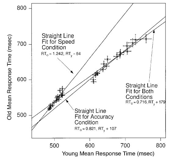
Brinley plots for correct response times (RTs) for the experiment. The points on the graph represent the same conditions for older and young subjects. Straight lines are fitted for speed and accuracy conditions separately and for the conditions combined. Error bars are two standard errors in mean RT.

The data points have 2 standard error bars plotted around them. For the speed plot and the accuracy plot, the straight lines fall within the error bars (or ellipses that could be drawn around them) for all but 3 or 4 out of 36 data points. In other words, the straight lines provide reasonably good descriptions of the data. However, when the speed and accuracy data are combined, the straight line misses the confidence ellipses for about 10 data points, indicating that the straight line does not provide an adequate description of the data. Although standard error bars are usually not presented for Brinley plots, the data in Figure 2 illustrate why they should be: In many cases in which data from different experiments or conditions are combined, a straight line may not provide a good fit to the data (see Ratcliff, Spieler, & McKoon, 2003).

Accuracy

Figure 3 shows plots of the probability of a bright response as a function of six levels of brightness and three stimulus presentation times for older and young subjects for the speed and the accuracy conditions. At the short stimulus duration, there is a bias toward responding bright, and at the long stimulus duration, there is a bias toward responding dark (see Ratcliff, 2002). If there were no bias, the three functions would pass through the cross hairs in the middle of the figure. The bias probably occurred because the neutral gray background was perceived as dark, as compared with the white in the stimulus, at the shortest stimulus duration. As will be seen below, this bias is treated exactly the same way in the diffusion model as bias is treated in signal detection theory, with a criterion on drift rate (Ratcliff, 1985; Ratcliff et al., 1999). For each stimulus presentation duration, response probability for the two brightest stimuli is about the same, and the effect of stimulus duration shows up for the darker stimuli.

Figure 3.

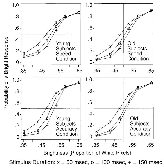
Probability of a bright response as a function of brightness of the stimulus for three stimulus durations and speed and accuracy conditions. The data are averaged over subjects.

Quantile probability functions

Quantitative models are needed to provide a complete explanation of processing in this task—that is, to account for all aspects of the experimental data. A model that deals only with correct mean RT is incomplete, since it cannot account for accuracy rates, error RTs, or the shapes of RT distributions. If a model for mean RTs only were extended, it would almost certainly make incorrect predictions. In contrast, the diffusion model provides an account of all the dependent variables in the decision process—correct and error RTs, their distributions, and accuracy rates. To fully test the diffusion model, it is fit simultaneously to all these aspects of the data, which are plotted as quantile probability functions (Figures 4 and 5).

Figure 4.

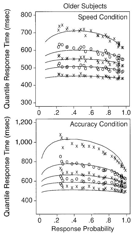
Quantile probability plots for older subjects. The lines represent the theoretical fits of the diffusion model, and the × s and ο s represent the data (vertically adjacent quantiles alternate with × and ο symbols). The lines in order from the bottom to the top are for the .1, .3, .5, .7, and .9 quantile response times (RTs). Correct responses are to the right of the .5 response probability point, and the corresponding error responses are to the left; if the correct response probability is p, the error response probability is 1 − p. Extreme errors (with a probability of less than about .2) are not represented because a sizable proportion of the subjects had fewer than five responses in these extreme conditions (five RTs are needed to compute five quantile RTs).

Figure 5.

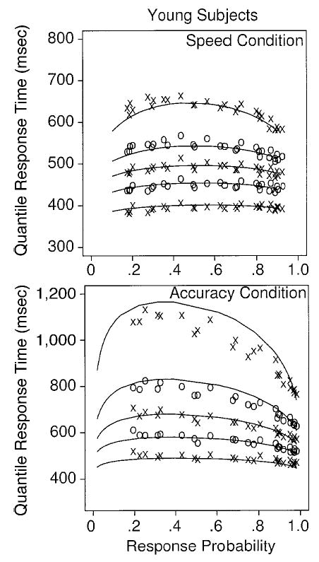
Quantile probability plots for young subjects. The lines represent the theoretical fits of the diffusion model, and the × s and ο s represent the data (vertically adjacent quantiles alternate with × and ο symbols). The lines in order from the bottom to the top are for the .1, .3, .5, .7, and .9 quantile response times (RTs). Correct responses are to the right of the .5 response probability point, and the corresponding error responses are to the left; if the correct response probability is p, the error response probability is 1 − p. Extreme errors (with a probability of less than about .2) are not represented because a sizable proportion of the subjects had fewer than five responses in these extreme conditions (five RTs are needed to compute five quantile RTs).

In quantile probability functions, response probabilities are shown on the x-axis, and quantile RTs are plotted vertically on the y-axis. For each condition of the experiment reported here, the .1, .3, .5 (median), .7, and .9 RT quantiles are plotted for both error responses and correct responses in Figures 4 and 5. The × s and ο s are data points (the × s for the .1, .5, .9 quantiles and the ο s for the .3 and .7 quantiles), and the lines are the best-fitting functions from the diffusion model, discussed below.

There were 36 conditions in the experiment: 3 stimulus duration conditions, 6 brightness conditions, and 2 speed and accuracy conditions. Responses for the bright and the dark stimuli were combined because their quantiles fell on the same function. For each of the 36 conditions, there are two probabilities: the probability of a correct response and the probability of an error (which equals 1 − the probability of a correct response). The subjects were generally above .5 in accuracy, and so the responses plotted on the right hand side of the quantile probability function are correct responses; the responses plotted on the left are errors. The function traces out the difficulty of the conditions: The easiest conditions are those with the most extreme left and right hand quantiles—that is, the quantiles with the highest probability of a correct response and the lowest probability of an error. As an example, the condition with high brightness, medium duration, and accuracy instructions has a probability correct of .875 and an error probability of .125.

For each of the conditions, there are about 3,600 observations for correct and error responses combined. For example, for a condition in which accuracy was .8, there were about 2,880 observations for correct responses and 720 for error responses, about 80 correct and 20 error responses per subject on average. However, the subjects varied considerably in their accuracy, and for the easiest conditions, some subjects’ accuracy was above .95, so that they had fewer than five errors, which means that they did not have the five RTs needed to plot the error quantile probability function. For this reason, quantile RTs are not plotted for errors for the easiest conditions (between three and seven quantiles are not plotted for the four plots in Figures 4 and 5).

The quantile probability function gives a summary picture of the data, including the shapes of the RT distributions. For both older and young subjects, RT increases and accuracy decreases as difficulty increases (i.e., as stimulus duration and brightness decrease), although the changes are smaller with speed than with accuracy instructions. The overall shapes of the RT distributions are about the same across all the conditions. The error RTs in each condition are longer than the correct response RTs for the same condition (as can be seen by comparing the correct RTs for a condition on the right side of the function against the error RTs for the same condition on the left side).

Responses are considerably faster with speed than with accuracy instructions, as is shown in Figures 4 and 5 for all quantile RTs. Responses are also more accurate with accuracy instructions, but the effect is small, between 0 and .05.

With accuracy instructions, for correct responses, the RT distribution skews out as stimulus difficulty increases. Across the conditions, the .1 quantile RTs increase a little, but the .9 quantiles increase much more, by as much as 300 msec. With speed instructions, the skewing is less apparent, with only about 100 msec of slowing in the .9 quantile for older subjects and a little less for young subjects.

Older subjects are slower than young subjects with speed instructions, by about 50 msec, but with accuracy instructions, they are about equally fast. If anything, the .1 quantile RTs are shorter for the young than for the older subjects, whereas the .9 quantile RTs are longer for the young. The older and young subjects were about equally accurate in both the speed and the accuracy conditions.

To summarize, in order to fit the data, the diffusion model has to produce moderately large changes in RT with small changes in accuracy going from speed to accuracy instructions. Accuracy decreases as brightness becomes less extreme and stimulus duration becomes smaller, and RT distributions have to be right skewed, with the spread in the tail greater for longer RTs, but with little change in the .1 quantile RT. The small changes in accuracy suggest that there may be little effect of aging on drift rates because accuracy values determine drift rates to a large degree. Because RTs are longer for older subjects in the speed condition, but not in the accuracy condition, the model fits may show that older subjects use more conservative criteria settings with speed instructions, but not with accuracy instructions.

DIFFUSION MODEL FITS

The diffusion model was fit to the data by minimizing a chi-square value with a general SIMPLEX minimization routine that adjusts the parameters of the model to find the parameters that give the minimum chi-square value. The data entered into the minimization routine for each experimental condition were the RTs for each of the five quantiles for correct and error responses and the accuracy values. The quantile RTs were fed into the diffusion model, and for each quantile, the cumulative probability of a response by that point in time was generated from the model. Subtracting the cumulative probabilities for each successive quantile from the next higher quantile gives the proportion of responses between each quantile. For the chisquare computation, these are the expected values, to be compared with the observed proportions of responses between the quantiles (multiplied by the number of observations). The observed proportions of responses for each quantile are the proportions of the distribution between successive quantiles (i.e., the proportions between 0, .1, .3, .5, .7, .9, and 1.0 are .1, .2, .2, .2, .2, and .1) multiplied by the probability correct for correct response distributions or the probability of error for error response distributions (in both cases, multiplied by the number of observations). Summing over (observed − expected)²/expected for all conditions gives a single chi-square value to be minimized (see Ratcliff & Tuerlinckx, 2002, for a detailed description).

Short outliers were trimmed out by choosing a time (250 msec for young subjects and 280msec for older subjects) at which accuracy began to rise above chance (e.g., Swensson, 1972) and long outliers (RTs longer than 3,000 msec for young subjects and 3,500 msec for older subjects) were also eliminated from the analyses. Ratcliff and Tuerlinckx (2002) modeled remaining contaminant RTs by assuming that they arose from a random delay added to the normal decision process. The delay was assumed to vary uniformly between the minimum and the maximum RTs in the condition, and there was a common probability of a contaminant across all conditions. This adds one additional parameter to the diffusion model (p_o) to represent the probability of a contaminant in each condition of the experiment. In the fits presented next, p_o was typically .01 or less, and so contaminants played little role.

For the fits presented here, five parameters were held constant across the 18 stimulus duration and brightness conditions and the speed versus accuracy instructions: p_o, T_er, s_t, s_z, and η (probability of a contaminant, nondecision component of RT, and across-trial variabilities in T_er, z, and drift rate, respectively). Holding these five parameters constant reflects the assumption that neither speed versus accuracy instructions nor the quality of the information from the stimulus affects any of these components of the decision process. The separation of the boundaries was assumed to be affected by the speed/accuracy manipulation, but not by brightness or stimulus duration (because it was assumed that subjects could not identify the stimulus duration or brightness in time to adjust criteria before making their decision). The drift rate was assumed to be affected by duration and brightness, but not by speed/accuracy instructions. Changes in drift rate move points along the quantile probability function but do not alter the shape of the function.

To reduce the number of parameters, we set the drift rates for complementary bright and dark stimuli to be complements of each other (e.g., bright drift rate equals minus dark drift rate). However, individual subjects were often biased on the brightness dimension (see Figure 3), and so we added a drift criterion for each stimulus duration (see Ratcliff, 1985, 2002; Ratcliff et al., 1999). The criterion value was added to the drift rate for all brightness values.

With these restrictions on parameters, the model must account for accuracy rates, the relative speeds of correct and error responses, and the shapes of the RT distributions. Specifically, with only boundary separation varying, the model must account for the small changes in accuracy and the large changes in RT between the speed and the accuracy conditions. With only drift rate varying, the model must account for the changes in accuracy and RT distribution shape for both errors and correct responses as a function of brightness and stimulus duration.

We fit the diffusion model to the data in two ways. First, each subject’s data were fit individually, and the parameter values were averaged across subjects. The means and standard deviations for each of the parameters are shown in Tables 2 and 3. Standard errors in the parameter values (for significance tests) can be found by dividing the standard deviations by the square root of the number of subjects. Second, we fit the model to the data averaged over all the subjects in a group (older vs. young subjects). These fits were used as the basis for the predictions displayed in Figures 4 and 5 (the solid lines). Group data have often been used in the fitting of models, and the assumption (usually implicit) is that the fits and parameter values for the group data will turn out to be the same as the averages from the fits for the individual subjects. We provide both for comparison. The parameter values obtained from the group data and the average parameter values across individuals are within two standard errors of each other for all parameters (see Tables 2 and 3). Also, the parameter

Table 2.

Parameters for Fits of the Diffusion Model

	as	aa	Ter	η	sz	po	st
Young fit to average data	0.072	0.128	0.406	0.124	0.030	.011	0.170
Young average parameters	0.073	0.135	0.405	0.151	0.037	.010	0.172
Young SDs in parameters	0.013	0.030	0.025	0.061	0.022	.006	0.046
Old fit to average data	0.071	0.116	0.459	0.155	0.033	.007	0.156
Old average parameters	0.074	0.122	0.448	0.156	0.030	.009	0.167
Old SDs in parameters	0.015	0.025	0.027	0.045	0.017	.004	0.037

Note—a_s, boundary separation for speed condition; a_a, boundary separation for accuracy condition; T_er, nondecision component of response time; η, standard deviation in drift across trials; s_z, range of the distribution of starting point (z); p_o, proportion of contaminants; and s_t, range of the distribution of nondecision times.

Table 3.

Drift Rates for Fits of the Diffusion Model

Brightness	Flash Time (msec)	Young Fit to Average Data	Young Means Over Subjects	Old Fit to Average Data	Old Means Over Subjects
.350 & .650	50	0.339	0.358	0.379	0.348
.425 & .575	50	0.192	0.212	0.234	0.217
.475 & .525	50	0.126	0.097	0.085	0.101
.350 & .650	100	0.356	0.410	0.428	0.433
.425 & .575	100	0.270	0.283	0.270	0.288
.475 & .525	100	0.117	0.104	0.102	0.100
.350 & .650	150	0.348	0.416	0.438	0.451
.425 & .575	150	0.267	0.309	0.263	0.329
.475 & .525	150	0.179	0.183	0.140	0.184
Bias (add to drift rates above)	50	0.066	0.059	0.046	0.048
	100	0.003	0.003	−0.026	−0.025
	150	−0.037	−0.027	−0.095	−0.045

Note—Standard deviations are .10 when drift rate is .35, .07 when drift rate is .25, and .05 when drift rate is .10. Drift rates are within 4% of each other for old and young for means over subjects (old are 4% higher than young) and within 1% for fits to average data. A single correlation of plus or minus .33 would be significant at a .05 level.

The fits (Figures 4 and 5) show that the model captures the changes in RT and accuracy as a function of stimulus duration, brightness, and speed versus accuracy instructions for both correct and error responses, as well as the overall differences between the older and the young subjects. The only noticeable misses are for the .9 quantile RTs with accuracy instructions (but these are not severe misses, given the high variability in longer RTs; see Ratcliff & Tuerlinckx, 2002). If subjects were to truncate their responses after 1.5–2 sec of processing on some proportion of the trials, the discrepancy in the .9 quantile in the accuracy condition would be reduced or eliminated. This might happen if the decision boundaries were reduced as processing time increased (cf. Luce, 1986, p. 375) or if the subjects simply truncated processing after some long variable time.

Analysis of the parameter estimates showed that the older subjects differed from the young subjects in only one way. The value of T_er was larger for older subjects than for young subjects by about 40–50 msec [t (69) = 4.93; this was computed from the values of T_er for the fits to the individual subjects]. This increase in T_er for older subjects relative to young subjects is about the same size increase in T_er as that found by Ratcliff et al. (2003) and Thapar et al. (in press). Drift rates and boundary separations for both the speed and the accuracy conditions were not significantly different between older and young subjects. Thus, the older subjects were obtaining stimulus information from the display at the same rate as the young subjects, and they were setting the same decision criteria as the young subjects.

We computed chi-square values for each subject in the process of fitting the model to data, and the mean values and SDs were χ² = 951, SD = 408, for young subjects (average number of observations = 4,735 per subject) and χ² = 680, SD = 320, for older subjects (average number of observations = 3,275 per subject). But as was noted in Ratcliff (2002), the diffusion model is much more constrained than might be expected from the number of parameters used in fitting. First, the nine drift rates and the three drift criterion parameters determine position along the x-axis of the quantile probability function. They do not influence the shapes of the quantile probability functions. Second, the value of T_er locates only the vertical positions of the quantile probability functions; it does not also influence their shape. Third, the estimate of the proportion of contaminant responses (p_o) is usually less than or near to .01 and has no effect on the predicted quantile probability functions relative to the case in which it is zero. Fourth, although variability in T_er (s_t) allows the .1 quantile response times to be more variable and more in line with the observed variability, its only effect on quantile RTs is a less than 7-msec increase in the difference between the .1 and the .3 quantile RTs. Fifth, the shape of the quantile probability functions is determined only by the parameters η (standard deviation in drift across trials), S_z (range of starting point across trials), and the values of boundary separation (a), one value for the speed conditions and one for the accuracy conditions. All the parameters except a were held constant across the speed and the accuracy data. Thus, the shape and location of the quantile probability functions are determined by only three parameters, with only one of them different for speed versus accuracy instructions.

Correlations between data and parameters across subjects

Figure 6 and Table 4 show scatterplots and correlations across subjects for mean values of accuracy, correct RTs, .1 quantile RTs for correct responses, error RTs, and the parameters of the diffusion model—the mean values of boundary separations, the nondecisional components of RT, and drift rates. The means for the data were averaged across all brightness, stimulus duration, and speed and accuracy conditions. The means for boundary separation and drift rate were computed by averaging across all conditions (after first checking that the two boundary separations for speed and accuracy instructions behaved in the same ways across subjects and that the nine drift rates behaved in the same ways across subjects).

Figure 6.

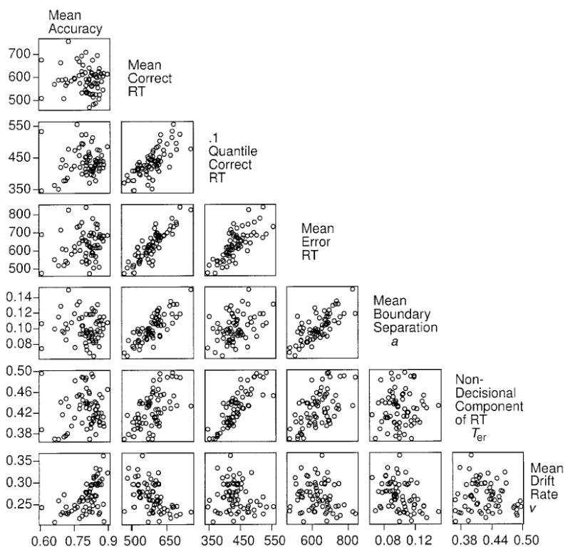
Scatterplots of accuracy, mean correct response time (RT), .1 quantile RT for correct responses, mean error RT, and, from fits of the diffusion model to the data, mean boundary separation (average of speed and accuracy settings), mean value of the nondecisional component of RT, and mean value of drift across conditions for all subjects (young and old) in the experiment.

Table 4.

Correlations Between Accuracy and Response Time (RT) Measures and Diffusion Model Parameters

	Accuracy	Mean Correct RT	Correct .1 Quantile RT	Mean Error RT	a	Ter	v
Accuracy	1.00	−.12	.13	.21	−0.07	05	.53
Mean Correct RT	−.12	1.00	.72	.88	.82	.56	−.52
Correct .1 Quantile RT	.13	.72	1.00	.75	.38	.83	−.16
Mean error RT	.21	.88	.75	1.00	.74	.57	−.21
a	−.07	0.82	.38	74	1.00	.09	−.39
Ter	.05	0.56	.83	.57	.08	1.00	−.12
V	.53	−.52	−.16	−.21	−.39	−.12	1.00

Note—a, boundary separation averaged over speed and accuracy conditions; T_er nondecision component of response time; and v, drift rate. A single correlation of .24 would be significant at a .05 level.

For the empirical measures, correct and error RTs are highly correlated, and both are slightly less correlated with .1 quantile RTs for correct responses. The correlation between accuracy and the RT measures is close to zero, indicating that a subject’s accuracy level does not predict his/her RTs.

There is only one correlation of note among the model parameters, a moderate negative correlation between drift rate and boundary separation, but inspection of the scatterplot in Figure 6 suggests that it is not particularly strong. All the other correlations are small.

There are a number of strong correlations between model parameters and empirical measures. First, there are strong correlations between boundary separation and the RT measures. This means that conservative boundary settings are reflected in long RTs. However, the correlation between boundary separation and accuracy is close to zero. Second, there is a moderately high correlation between drift rate and accuracy, which means that low accuracy reflects a low drift rate—that is, a slow rate of evidence accumulation. Third, there is a moderately high negative correlation between drift rate and correct RTs, which means that slower subjects tend to have lower drift rates. Fourth, there is a strong correlation between the nondecisional component of RT and the .1 quantile RT and a lower correlation between the nondecisional component of RT and RTs.

The only correlation of any note that is not displayed in Table 4 or Figure 6 is the one between standard deviation in drift across trials (η) and accuracy, a value of −.57. This indicates that accurate subjects tend to have small standard deviations in drift across trials.

The most concise summary of these results is that, across subjects, accuracy tends to be associated with drift rate and RTs tend to be associated with boundary separation and the nondecisional component of RT, although the latter two are not associated. This suggests that accuracy and RT values are determined by different factors in the diffusion model. If a subject is accurate relative to other subjects, the subject’s drift rates are higher than those for the other subjects, whereas if a subject is faster than other subjects, the subject’s boundary separations are smaller than those for the other subjects.

GENERAL DISCUSSION

The results from this study are remarkable. Older subjects perform just as well as young subjects in all aspects of performance in brightness discrimination, except that processes other than those directly involved in the decision take 40–50 msec longer. There was no deficit in the rate of extraction of information from the stimuli (drift rates) for the older subjects, and they were not more conservative in their criteria settings.

These results have some similarity to those obtained by Ratcliff et al. (2001) in a signal detection-like task. Ratcliff et al. (2001) found a 40- to 50-msec difference in the nondecision component of RT between older and young subjects and no deficit in drift rate. However, in contrast to the present study, they also found that older subjects adopted more conservative decision criteria than did young subjects in both speed and accuracy conditions.

The present study contrasts in two ways to Thapar et al.’s (in press) study, in which masked letter discrimination was examined. Although Thapar et al. found about the same difference in nondecision components of RT, they found both more conservative decision criteria for older subjects than for young subjects and a deficit in the rate of accumulation of evidence for older subjects, as compared with young subjects. The difference in results is surprising at a cursory level because masked-letter discrimination and masked brightness discrimination are similar perceptual tasks. However, as was discussed in the introduction, the perceptual literature (e.g., Spear, 1993) provides evidence that with stimuli with high spatial frequencies, such as letters, older adults have deficits in identification, relative to young subjects, whereas with low spatial frequency stimuli, such as the stimuli in this experiment, there are no deficits as a function of aging for our age range (deficits appear in 75- to 90-year-olds). Thus, application of the diffusion model to the data from this experiment and Thapar et al.’s experiment provides an account of the effects of aging on two different perceptual tasks that is highly consistent with the perceptual literature. In particular, the drift rate in the diffusion model, which represents the accumulation of evidence from the stimulus, shows the same effect of aging as that obtained from other paradigms that use only accuracy, not RT, measures. The diffusion model is a model of the decision process, and so it is able to identify a deficit in the quality of evidence presented by the visual-processing system to the decision process, but it is not able to identify where in visual processing the deficit occurs.

As the diffusion model is applied to a variety of tasks, patterns of results are becoming apparent that allow rates of extraction of information from stimuli (as represented by drift rates in the model) to be decoupled from nondecision components of RT and from criterion effects (just as signal strength is decoupled from criterion in signal detection theory). Instead of a monolithic account of processing speed solely in terms of mean correct RT, as has been popular in the general slowing approach to aging, we have a componential account in terms of information extracted from the stimulus and subject-adjustable decision criteria, an account that encompasses correct and error RTs, their distributions, and accuracy. The three studies conducted so far—this one, Ratcliff et al. (2001), and Thapar et al. (in press)—also indicate that the measure of information extraction (drift rate) matches well with results obtained using other measures, such as accuracy or threshold values. Finally, the good fits of the model add to a growing body of results that support the diffusion model as an explanation of two-choice decision processes and provide evidence of the generality of the model across experimental paradigms.

References

- Brinley, J. F. (1965). Cognitive sets, speed and accuracy of performance in the elderly. In A.T. Welford & J. E. Birren (Eds.), Behavior, aging and the nervous system (pp. 114–149). Springfield, IL: Thomas.
- Busemeyer JR, Townsend JT. Decision field theory: A dynamic-cognitive approach to decision making in an uncertain environment. Psychological Review. 1993;100:432–459. doi: 10.1037/0033-295x.100.3.432. [DOI] [PubMed] [Google Scholar]
- Cerella J. Information processing rates in the elderly. Psychological Bulletin. 1985;98:67–83. [PubMed] [Google Scholar]
- C erella, J. (1990). Aging and information-processing rate. In J. E. Birren & K. W. Schaie (Eds.), Handbook of the psychology of aging (3rd ed., pp. 201–221). San Diego: Academic Press.
- Cerella J. Age effects may be global, not local: Comment on Fisk and Rogers (1991) Journal of Experimental Psychology: General. 1991;120:215–223. doi: 10.1037/0096-3445.120.2.215. [DOI] [PubMed] [Google Scholar]
- Cerella J. Generalized slowing in Brinley plots. Journal of Gerontology: Psychological Sciences. 1994;49:65–71. doi: 10.1093/geronj/49.2.p65. [DOI] [PubMed] [Google Scholar]
- Coyne AC. Age difference and practice in forward visual masking. Journal of Gerontology. 1981;36:730–732. doi: 10.1093/geronj/36.6.730. [DOI] [PubMed] [Google Scholar]
- Elliott D, Whitaker D, MacVeigh D. Neural contribution to spatiotemporal contrast sensitivity decline in healthy aging eyes. Vision Research. 1990;30:541–547. doi: 10.1016/0042-6989(90)90066-t. [DOI] [PubMed] [Google Scholar]
- Fisher DL, Glaser RA. Molar and latent models of cognitive slowing: Implications for aging, dementia, depression, development, and intelligence. Psychonomic Bulletin & Review. 1996;3:458–480. doi: 10.3758/BF03214549. [DOI] [PubMed] [Google Scholar]
- Fisk JE, Warr P. Age and working memory: The role of perceptual speed, the central executive, and the phonological loop. Psychology & Aging. 1996;11:316–323. doi: 10.1037//0882-7974.11.2.316. [DOI] [PubMed] [Google Scholar]
- Folstein MF, Folstein SE, McHugh PR. Minimental state: A practical method for grading the cognitive state of patients for the clinician. Journal of Psychiatric Research. 1975;12:189–198. doi: 10.1016/0022-3956(75)90026-6. [DOI] [PubMed] [Google Scholar]
- F ozard, J. L. (1990). Vision and hearing in aging. In J. E. Birren & K. W. Schaie (Eds.), Handbook of the psychology of aging (pp. 150–170). San Diego: Academic Press.
- L uce, R. D. (1986). Response times New York: Oxford University Press.
- Myerson J, Hale S, Wagstaff D, Poon LW, Smith GA. The information-loss model: A mathematical theory of age-related cognitive slowing. Psychological Review. 1990;97:475–487. doi: 10.1037/0033-295x.97.4.475. [DOI] [PubMed] [Google Scholar]
- Owsley C, Sekuler R, Siemsen D. Contrast sensitivity through adulthood. Vision Research. 1983;23:689–699. doi: 10.1016/0042-6989(83)90210-9. [DOI] [PubMed] [Google Scholar]
- Radloff LS. The CES–D Scale: A self-report depression scale for research in the general population. Applied Psychological Measurement. 1977;1:385–401. [Google Scholar]
- Ratcliff R. A theory of memory retrieval. Psychological Review. 1978;85:59–108. [Google Scholar]
- Ratcliff R. A theory of order relations in perceptual matching. Psychological Review. 1981;88:552–572. [Google Scholar]
- Ratcliff R. Theoretical interpretations of speed and accuracy of positive and negative responses. Psychological Review. 1985;92:212–225. [PubMed] [Google Scholar]
- Ratcliff R. Continuous versus discrete information processing: Modeling the accumulation of partial information. Psychological Review. 1988;95:238–255. doi: 10.1037/0033-295x.95.2.238. [DOI] [PubMed] [Google Scholar]
- Ratcliff R. A diffusion model account of response time and accuracy in a brightness discrimination task: Fitting real data and failing to fit fake but plausible data. Psychonomic Bulletin & Review. 2002;9:278–291. doi: 10.3758/bf03196283. [DOI] [PubMed] [Google Scholar]
- R atcliff, R., Gomez, P., & McKoon, G. (in press). Diffusion model account of the lexical decision task Manuscript submitted for publication. [DOI] [PMC free article] [PubMed]
- Ratcliff R, Rouder JF. Modeling response times for two-choice decisions. Psychological Science. 1998;9:347–356. [Google Scholar]
- Ratcliff R, Rouder JF. A diffusion model account of masking in two-choice letter identification. Journal of Experimental Psychology: Human Perception & Performance. 2000;26:127–140. doi: 10.1037//0096-1523.26.1.127. [DOI] [PubMed] [Google Scholar]
- Ratcliff R, Spieler D, McKoon G. Explicitly modeling the effects of aging on response time. Psychonomic Bulletin & Review. 2000;7:1–25. doi: 10.3758/bf03210723. [DOI] [PubMed] [Google Scholar]
- R atcliff, R., Spieler, D., & McKoon, G. (2003). Analysis of group differences in processing speed: Where are the models of processing? Manuscript submitted for publication. [DOI] [PMC free article] [PubMed]
- Ratcliff R, Thapar A, McKoon G. The effects of aging on reaction time in a signal detection task. Psychology & Aging. 2001;16:323–341. [PubMed] [Google Scholar]
- Ratcliff R, Tuerlinckx F. Estimating parameters of the diffusion model: Approaches to dealing with contaminant reaction times and parameter variability. Psychonomic Bulletin & Review. 2002;9:438–481. doi: 10.3758/bf03196302. [DOI] [PMC free article] [PubMed] [Google Scholar]
- Ratcliff R, Van Zandt T, McKoon G. Connectionist and diffusion models of reaction time. Psychological Review. 1999;106:261–300. doi: 10.1037/0033-295x.106.2.261. [DOI] [PubMed] [Google Scholar]
- Roe RM, Busemeyer JR, Townsend JT. Multialternative decision field theory: A dynamic artificial neural network model of decision-making. Psychological Review. 2001;108:370–392. doi: 10.1037/0033-295x.108.2.370. [DOI] [PubMed] [Google Scholar]
- S althouse, T. A. (1985). A theory of cognitive aging Amsterdam: North-Holland.
- Salthouse TA. The processing-speed theory of adult age differences in cognition. Psychological Review. 1996;103:403–428. doi: 10.1037/0033-295x.103.3.403. [DOI] [PubMed] [Google Scholar]
- Salthouse TA, Kausler DH, Saults JS. Utilization of path-analytic procedures to investigate the role of processing resources in cognitive aging. Psychology & Aging. 1988;3:158–166. doi: 10.1037//0882-7974.3.2.158. [DOI] [PubMed] [Google Scholar]
- Smith PL. Psychophysically principled models of visual simple reaction time. Psychological Review. 1995;102:567–591. [Google Scholar]
- Spear PD. Minireview: Neural bases of visual deficits during aging. Vision Research. 1993;33:2589–2609. doi: 10.1016/0042-6989(93)90218-l. [DOI] [PubMed] [Google Scholar]
- Swensson RG. The elusive tradeoff: Speed vs. accuracy in visual discrimination tasks. Perception & Psychophysics. 1972;12:16–32. [Google Scholar]
- T hapar, A., Ratcliff, R., & McKoon, G. (in press). A diffusion model analysis of the effects of aging on letter discrimination. Psychology & Aging [DOI] [PMC free article] [PubMed]