

Abstract
Objective
To estimate the effect of survey mode (mail versus telephone) on reports and ratings of hospital care.
Data Sources/Study Setting
The total sample included 20,826 patients discharged from a group of 24 distinct hospitals in three states (Arizona, Maryland, New York). We collected CAHPS® data in 2003 by mail and telephone from 9,504 patients, of whom 39 percent responded by telephone and 61 percent by mail.
Study Design
We estimated mode effects in an observational design, using both propensity score blocking and (ordered) logistic regression on covariates. We used variables derived from administrative data (either included as covariates in the regression function or used in estimating the propensity score) grouped in three categories: individual characteristics, characteristics of the stay and hospital, and survey administration variables.
Data Collection/Extraction Methods
We mailed a 66-item questionnaire to everyone in the sample and followed up by telephone with those who did not respond.
Principal Findings
We found significant (p<.01) mode effects for 13 of the 21 questions examined in this study. The maximum magnitude of the survey mode effect was an 11 percentage-point difference in the probability of a “yes” response to one of the survey questions. Telephone respondents were more likely to rate care positively and health status negatively, compared with mail respondents. Standard regression-based case-mix adjustment captured much of the mode effects detected by propensity score techniques in this application.
Conclusions
Telephone mode increases the propensity for more favorable evaluations of care for more than half of the items examined. This suggests that mode of administration should be standardized or carefully adjusted for. Alternatively, further item development may minimize the sensitivity of items to mode of data collection.
Keywords: Patient evaluations of hospital care, CAHPS, propensity score, mode effects
The Consumer Assessment of Health Providers and Systems (CAHPS®) Hospital Survey assesses patients' experiences with care in the hospital. The survey was designed to be administered by mail or telephone to allow flexibility of administration and maximize response rates (Hochstim 1967; Dillman 2000). A hospital may choose to use one mode or the other to collect data or it may choose to use both (mixed mode). In either case, patients' responses could differ by the mode of administration (mode effect) because of different levels of interviewer involvement, interaction with the respondent, privacy, channels of communication (including primacy and recency effects), and use of technology (Groves et al. 2004).
Fowler, Gallagher, and Nederend (1999) found statistically significant mode effects for 9 of 58 patient evaluations of ambulatory care. The largest mode effect was a 15 percentage-point change in the probability of a particular answer. Hepner, Brown, and Hays (2005) found only one significant mode difference in item and composite means for the CAHPS Group Survey.
Mode effects have been estimated in a variety of ways, including observational studies (e.g., Criqui, Barrett-Connor, and Austin 1978; Brambilla and McKinlay 1987), randomized experiments, and repeated-measure studies in which the same individual sequentially responds to both modes (e.g., Acree et al. 1999; Brøgger et al. 2002). Groves et al. (2004) describe a continuum of mode comparison study designs, ranging from more practical to more theoretical. This paper falls on the more practical side of this continuum, as we estimate mode effects using a design where only nonrespondents to an initial mail survey were approached by telephone. This study design is commonly used in real-world settings because the intent of employing two modes is to maximize response rate by following nonresponders with the alternate mode rather than implement the preferred randomized experimental design for scientific purposes. By using statistical models including the propensity score, our observational design mimics the randomized experiment as closely as possible with a given set of covariates. As such, we believe our findings are of particular interest to those interested in the estimation of mode effects in practical settings.
The mode effect can be decomposed into multiple separate effects, associated with differences in sampling frames, population coverage, nonresponse, and measurement quality between the two modes (Groves et al. 2004). In this paper we are primarily interested in aspects of measurement quality, such as bias caused by socially desirable responses. Nonresponse is addressed in a separate article in this issue (Elliott et al. 2005).
DATA
Our data are derived from the administration of the original 66-item field test questionnaire, but only questions in the 32-item version were analyzed here because this is a closer approximation to the final version of the survey the Centers for Medicare and Medicaid Services (CMS) is expected to adopt for national implementation.1 Of these 32 questions, 11 did not qualify for the analysis: three that have subsequently been reworded substantially (14, 17, and 19); four that were omitted from the telephone mode (31 and 32 by design; 15 and 16 because of a skip pattern error); three demographic characteristics (main language, race/ethnicity, questions 28, 29, and 30); and one discharge destination (question 20). These last four items were excluded because we had no a priori expectation of a mode effect. Except for question 4, the text of all 21 questions (and their response categories) included in our analysis is identical between the original and the 32-item questionnaire. A “not applicable” response category (“I never pressed the call button”) was added for question 4.
The dataset represents patients who stayed in any of 24 hospitals. The sample included 20,826 discharges of which 9,504 responded. Data collection by telephone targeted only those patients who had not responded to the mail survey within 1 month. The time between the day the survey was mailed out and the day response was received was on average 28 days for mail respondents and 48 days for telephone respondents. In order to distinguish effects of mode itself from effects associated with delayed response, we compare telephone respondents first to all mail respondents and then specifically to late mail respondents (i.e., the 29 percent of mail respondents who completed the survey more than 30 days after it was mailed out). The average lag time for the 1,714 late mail respondents (45 days) is fairly close to that of telephone respondents. Late mail respondents (panel c of Table 1) resembled phone respondents more closely (compared with all mail respondents) with respect to age, gender, race (black and white categories), and days since discharge. Additional details about the data collection process are given elsewhere (Goldstein et al. 2005).
Table 1.
Characteristics of Telephone and Mail Respondents
| Covariate | (a) All Phone Respondents | (b) All Mail Respondents | (c) Mail Respondents >30 Days | (d) Nonrespondents |
|---|---|---|---|---|
| Mean age | 50.20 | 54.64** | 50.62 | 48.52** |
| % Spanish language | 9.12 | 2.95** | 1.75** | N/a |
| % Female | 69.28 | 66.53** | 71.88 | 65.11** |
| % White | 59.18 | 68.40** | 64.82** | 53.25** |
| % Black | 10.39 | 6.16** | 8.93* | 14.69** |
| % Asian | 1.14 | 1.10 | 1.28 | 2.32** |
| % Hispanic | 13.74 | 6.36** | 5.72** | 12.18** |
| % NA Native | 0.71 | 0.38* | 0.53 | 0.97** |
| % Unknown | 7.35 | 6.33 | 6.88 | 8.20** |
| % Missing | 7.48 | 11.27** | 11.84** | 8.39** |
| Mean length of stay (days) | 3.73 | 3.81 | 3.79 | 3.84 |
| Mean days since discharge | 165.85 | 164.84* | 165.56 | |
| % Discharge status: home | 89.52 | 89.91 | 91.07 | 89.98 |
| % Discharge status: still sick | 9.63 | 9.66 | 8.40 | 8.96 |
| % Discharge status: walked out | 0.44 | 0.12** | 0.18 | 0.83** |
| % Discharge status: other | 0.41 | 0.41 | 0.35 | 0.24* |
| % Standard referral | 58.69 | 63.32** | 64.94** | 57.30** |
| % Transfer | 2.94 | 2.66 | 3.09 | 2.62 |
| % ER | 27.86 | 24.76** | 22.81** | 31.10** |
| % Other | 10.50 | 9.26* | 9.16 | 8.97 |
| % Medical | 36.33 | 33.93* | 31.80** | 39.81** |
| % Surgical | 35.40 | 41.91** | 38.10 | 30.64** |
| % Obstetrics | 28.27 | 24.16** | 30.11 | 29.55** |
| % MDC: nervous system | 4.84 | 5.22 | 4.90 | 5.18 |
| % MDC: ENT, mouth | 1.14 | 0.89 | 0.99 | 1.12 |
| % MDC: respiratory system | 5.47 | 6.60* | 5.72 | 7.45** |
| % MDC: circulatory system | 18.72 | 18.82 | 15.64** | 16.23** |
| % MDC: digestive system | 9.71 | 10.02 | 9.80 | 9.34 |
| % MDC: liver/pancreas system | 3.37 | 2.57* | 2.10** | 2.94 |
| % MDC: musculoskeletal system | 7.05 | 10.38** | 10.27** | 7.62** |
| % MDC: skin/subcutissue/breast | 2.59 | 2.30 | 2.28 | 2.59 |
| % MDC: metabolic disorders | 2.64 | 2.37 | 1.69* | 2.60 |
| % MDC: kidney/urinary tract | 3.21 | 2.78 | 2.68 | 3.15 |
| % MDC: male reproductive | 0.79 | 1.27* | 0.93 | 0.79* |
| % MDC: female reproductive | 4.73 | 5.35 | 5.89* | 3.36** |
| % MDC: preg/chbrth/puerperium | 28.27 | 24.16** | 30.11 | 29.56** |
| % MDC: infectious diseases | 1.01 | 1.17 | 1.40 | 1.04 |
| % MDC: injury/poisoning | 1.09 | 1.13 | 1.11 | 1.75 |
| % MDC: health status/health srvcs | 2.01 | 2.42 | 2.33 | 1.71** |
| % MDC: other | 3.35 | 2.56* | 2.16* | 3.56** |
Panels b and c significantly different from telephone mode respondents at .05 level; panel d significantly different from all respondents at .05 level
Panels b and c significantly different from telephone mode respondents at .01 level; panel d significantly different from all respondents at .01 level
The administrative data shown in Table 1 had no missing values, except for race. In case of missing values for items on the questionnaire with an ordered response format, we imputed values under Missing at Random assumptions (Rubin 1976) using SAS software (PROC MI). Such imputations might be interpreted as predictions of the responses that might have been expected from these respondents had they appropriately answered the skipped items, using relationships observed among those who actually answered those items.
METHOD
We test the null hypothesis that mode (mail versus telephone) has no effect on the response by estimating 21 separate average treatment effects (ATE) for the 21 questions on the CAHPS Hospital Survey noted above.2 As respondents were not randomly assigned to mode, regressing the outcome of a question on mode could lead to unobserved variable bias. However, various methods have been developed to reduce this bias, under the assumption that the “treatment” (mode) satisfies some form of exogeneity.3,4 One such method is propensity score blocking, developed by Rosenbaum and Rubin (1983). In this analysis we use both regression on covariates and propensity score blocking to assess the possibility of mode effects in the CAHPS Hospital Survey data. The latter approach has the advantage of requiring weaker assumptions regarding functional forms and distributions. Analyses were conducted using Stata 8.2 statistical software.
Both approaches use three categories of independent (“pretreatment”) variables derived from administrative data: individual characteristics (age, language, gender, and race); characteristics of the stay and hospital (source of admission, length of stay, destination after discharge, medical service Diagnosis Related Group [DRG], and 24 hospital identifiers/23 dummy variables); and survey administration variables (the number of days between discharge and the date the first mail survey was sent out). Possible categories for the source of admission were standard referral, transfer, emergency room, and other. Possible types of medical service were medical, surgical, or obstetrics. DRGs were grouped into 17 standard categories.
Panels a–c of Table 1 describe mail and phone respondents with respect to these covariates. In order to estimate the ATE for a survey question, we assume it to be constant for all respondents (nonheterogeneity). We used logistic regression analyses to estimate ATEs for questions 12, 18, 21, and 22, which have a dichotomous yes (1)/no (0) response. We used ordered logistic regression analysis to estimate ATEs for questions 1–4, 6–8, 10, 11, and 13, which have four ordered response choices (never, sometimes, usually, always) and for question 5, 9, and 23, which use a 0–10 (11 category) ordinal response scale. We report robust standard errors to take into account within-hospital correlation—that is, to take into consideration that patients in the same hospital may be more similar than patients at different hospitals (Rogers 1993; Williams 2000; Wooldridge 2002).
Regression on Covariates
We used regression analysis to examine the impact of mode on responses to each of the survey questions, while controlling for the set of covariates shown in Table 1. All covariates were included as main effects, regardless of their level of statistical significance. We conducted sensitivity tests by adding to the model: (1) higher-order polynomials (squares and cubes) of age, length of stay, and the number of days between discharge and the date the survey was sent; (2) two-way interactions between covariates; and (3) additional respondent characteristics obtained from the survey itself. We examined the results of these regression analyses to assess the importance of mode effect in comparison with the effects of other variables.
Propensity Score Blocking
We also estimated ATEs using propensity score blocking, which mimics the properties of a randomized experiment. If respondents were randomly assigned to two groups representing mail and telephone mode, we would expect to find, on average, similar respondents across the two groups, which would guarantee no bias. To mimic this situation we split our dataset into a number of blocks that have on average similar respondents across the two groups (mail and telephone) within each block. We assess the extent to which respondent characteristics are “balanced” (i.e., resembling what we would expect to find in a randomized experiment) in each block by producing a table similar to Table 1 for each block, evaluating and iterating until balance is achieved. Finally, the overall ATE is estimated as weighted average of the ATEs within each block.
More specifically, the algorithm to split the data into blocks consists of the following steps. First, we estimate the propensity score, the conditional probability of receiving the treatment (i.e., responding by phone) by logistic regression of mode on the “pretreatment” variables. As such, respondents with similar propensity scores have on average similar values for the set of observed covariates. Then we split the dataset into two blocks at the median of the propensity score distribution. In each block we test whether the mean propensity score differs between mail and phone respondents; if so we split the block into two new blocks at the median propensity score of the block in question. As soon as all blocks are balanced with respect to the propensity score, we do a final test and estimate within each block whether the mean for each pretreatment variable differs by mode (see Rosenbaum and Rubin 1983, for a more extensive description of this algorithm, including proofs).
Evaluation of the Balancing Requirement for Propensity Score Blocking
Our estimates of the mode effect using propensity score blocking are valid only under the assumption that the blocks are well balanced—that the distribution of each pretreatment variable is identical for both modes within each block obtained through the algorithm described in the method section. We evaluated this by testing for a difference in means between survey and telephone mode for each pretreatment variable within each block. The algorithm produced a total number of eight blocks (mimicking eight separate randomized experiments), when we included all pretreatment variables shown in Table 1. Within the resulting set of 512 potential differences, we found 13 significant at the p <.05 level (eight blocks times 64 indicators). This is fewer than the 24 that would be expected by chance alone. When including higher order moments (squares) for age and length of stay, in addition to full two-way interactions between hospital and DRG indicators, we obtained 30 significant (p <.05) results from 8,024 potential differences (17 blocks times 472 variables and interactions), which is also fewer than what would be expected by chance. Thus, the balancing requirement is not violated. The mode effect estimates presented in Table 2 are based on the latter specification of the propensity score.
Table 2.
Effect of Telephone (Relative to Mail) Survey Mode on Survey Response
| Logistic Regression on Covariates | Propensity Score Blocking | ||||||||
|---|---|---|---|---|---|---|---|---|---|
| (a) Only Including Covariates from Administrative Data | (b) Including Questions 25–27 as Additional Covariates | (c) Including All Mail Respondents | (d) Only Including Mail Responses Past 29 Days | ||||||
| # | Question | Odds Ratio | SE | Odds Ratio | SE | Odds Ratio | SE | Odds Ratio | SE |
| Dichotomous | |||||||||
| 12 | Bathroom | 0.945 | 0.036 | 0.921 | 0.037* | 0.964 | 0.045 | 0.957 | 0.062 |
| 18 | New rx | 0.636 | 0.037** | 0.634 | 0.036** | 0.653 | 0.029** | 0.702 | 0.050** |
| 21 | Help after discharge | 1.056 | 0.082 | 1.098 | 0.095 | 1.094 | 0.084 | 1.155 | 0.115 |
| 22 | Writing symptoms | 1.029 | 0.059 | 1.060 | 0.064 | 1.064 | 0.067 | 1.086 | 0.089 |
| Ordered CAHPSoutcomes | |||||||||
| 1 | Respect | 1.326 | 0.052** | 1.374 | 0.056** | 1.336 | 0.063** | 1.435 | 0.094** |
| 2 | Listen | 1.253 | 0.054** | 1.256 | 0.060** | 1.271 | 0.055** | 1.273 | 0.085** |
| 3 | Explain things | 1.177 | 0.050** | 1.187 | 0.056** | 1.205 | 0.056** | 1.262 | 0.079** |
| 4 | Call help frequency | 1.196 | 0.060** | 1.217 | 0.067** | 1.206 | 0.054** | 1.283 | 0.080** |
| 6 | MD respect | 0.962 | 0.046 | 0.956 | 0.046 | 0.952 | 0.049 | 1.035 | 0.079 |
| 7 | MD listen | 1.106 | 0.052* | 1.115 | 0.055* | 1.116 | 0.053* | 1.153 | 0.077* |
| 8 | MD explain | 1.057 | 0.057 | 1.062 | 0.053 | 1.076 | 0.046 | 1.108 | 0.068 |
| 10 | Room clean | 1.488 | 0.074** | 1.496 | 0.082** | 1.495 | 0.068** | 1.427 | 0.091** |
| 11 | Room quiet | 1.427 | 0.090** | 1.414 | 0.087** | 1.433 | 0.058** | 1.437 | 0.087** |
| 13 | How often bathroom | 1.216 | 0.049** | 1.249 | 0.057** | 1.234 | 0.051** | 1.261 | 0.080** |
| 24 | Recommend hospital | 1.226 | 0.055** | 1.257 | 0.054** | 1.263 | 0.060** | 1.287 | 0.089** |
| Ordered patient characteristics | |||||||||
| 25 | Overall health | 1.344 | 0.053** | 1.242 | 0.051** | 1.251 | 0.071** | ||
| 26 | Overall mental health | 1.302 | 0.046** | 1.245 | 0.052** | 1.205 | 0.074** | ||
| 27 | Education level | 0.766 | 0.025** | 0.787 | 0.031** | 0.751 | 0.047** | ||
| Ordered 0–10 Ratings | |||||||||
| 5 | Rate nurses | 1.065 | 0.038 | 1.060 | 0.043 | 1.090 | 0.042* | 1.162 | 0.079* |
| 9 | Rate MD | 1.025 | 0.04 | 1.034 | 0.043 | 1.034 | 0.042 | 1.124 | 0.080 |
| 23 | Rating of hospital | 1.094 | 0.031** | 1.091 | 0.040* | 1.122 | 0.042** | 1.210 | 0.087** |
| Composites (0–100 scale)† | Coefficient | SE | Coefficient | SE | Coefficient | SE | Coefficient | SE | |
| Communication with nurse | 1.406 | 0.344** | 1.594 | 0.368** | 1.594 | 0.423** | 2.492 | 0.696** | |
| Communication with doctors | −0.803 | 0.44 | −0.680 | 0.392 | −0.835 | 0.450 | −0.157 | 0.724 | |
| Nursing services | 2.517 | 0.591** | 2.887 | 0.656** | 2.665 | 0.546** | 3.909 | 0.937** | |
| Discharge information | −1.194 | 0.822 | −1.617 | 0.894 | −1.588 | 0.844 | −2.302 | 1.307 | |
| Physical environment | 3.977 | 0.652** | 3.974 | 0.649** | 4.042 | 0.467** | 3.920 | 0.761** | |
Significant at p =.05 level
Significant at p =.01 level
Using a linear regression model instead of ordered logistic regression
RESULTS
We show our results in Table 2, where each column represents a different set of models: Column a presents results from regression on covariates, and column c presents comparable results from propensity score blocking. Columns b and d represent different specifications of the analysis. Inclusion of questions 25–27 as covariates is reported only for the regression on covariates (column b). Results of limiting the analysis to response past 29 days is reported only for the propensity score (column d). In the upper four panels of Table 2, we show odds ratios (ORs), representing the odds of being in a higher response category when answering by phone compared with mail. An OR of 1 means that mail and telephone respondents do not differ in their response, while an OR greater than 1 means that telephone respondents chose higher response categories compared with mail respondents. In the lower panel, we show regression coefficients for the composite scores, which reflect differences in the means of composite scores between mail and telephone respondents.
Dichotomous Questions
The upper-most panel of Table 2 shows a significant mode effect for one of the four questions with a dichotomous (yes/no) response format. This is for a screening question that asks whether the respondent received any medicine that (s)he had not taken before (question 18). With an OR of 0.64, the magnitude of the mode effect is considerable for this question—the odds of answering “yes” to question 18 for a telephone mode respondent are 0.64 times those for a similar mail mode respondent. The mode effect for this question is about the same using regression on covariates compared with propensity score blocking, although limiting the dataset to late respondents causes a slight decrease in the magnitude of the effect.
Ordered Questions and Ratings
Using regression on covariates (Table 2, column a, middle panels) we find that the mode effect is significant for 12 of the 17 questions with an ordered response format. For question 1–4, 10, 11, 13 (reports of care with the never/sometimes/usually/always format), responding by telephone leads to a more favorable evaluation of care, where the largest effect is found for question 10 (clean room and bathroom). Telephone mode respondents also tend to be more positive on recommending the hospital to friends and family (question 24), but rate their overall and mental health lower (questions 25 and 26 have a five point scale ranging from excellent to poor). Finally, telephone mode respondents report a lower education level (question 27). The findings for these last three questions are not what one would expect if telephone respondents are more likely than mail respondents to alter their answers toward more socially desirable responses. In particular, question 27 could be interpreted as reflecting true differences between telephone and survey respondents, rather than a mode effect, as education level is not included in our pretreatment variables.5 In fact, these three questions are recommended for case-mix adjustment in usage of the CAHPS Hospital Survey (O'Malley et al. 2005). Therefore we show results of mode effects for the other questions when including questions 25–27 as covariates in the model (Table 2, column b). When including self-reported (mental) health and education, we see a very small increase in the magnitude of the mode effect for the majority of the questions (maximum absolute difference in ORs for ordered outcomes is 0.046; median of absolute differences in OR is 0.010).
The mode effect is very small and not significant for two of the three 0–10 global rating items representing care received from nurses, doctors, and the hospital (questions 5, 9, and 23). This is unexpected, in that the report items are usually considered more objective and less subject to response biases than the global ratings. Here we find the opposite pattern.
Estimating the mode effect for these questions with propensity score blocking (Table 2, column c) causes very small changes in point estimates, suggesting the bias in regression on covariates may be minimal. For those items that ask for an evaluation of care, the magnitude of the effect increases slightly, when comparing propensity score blocking to regression on covariates and including all mail respondents. For the other items (health status and education) it decreases slightly. If only late mail respondents are included (Table 2, column d), we see a substantial increase in the size of the effect for most questions, except for question 18 (having received medicines that were not taken before), and question 10 (how often room and bathroom were kept clean), where we see a decrease.
CAHPS Hospital Survey Composites
We calculated (unweighted) composite scores on a 0–100 scale by grouping individual report items across the following themes, according to the seven-factor composite structure described in Keller et al. (2005): communication with nurse (questions 1, 2, and 3); communication with doctors (question 6, 7, and 8); nursing services (questions 4 and 13); discharge information (questions 21 and 22); and physical environment (questions 10 and 11). We did not calculate scores for the two remaining composites, because of limitations to our dataset described above. The lower panel of Table 2 shows that significant mode effects exist for three of the five composites: communication with nurse, nursing services, and physical environment. When estimating mode effects using the propensity score and including only late mail respondents, the mode effect increases substantially for the former two. Using regression on covariates, the largest effect is found for the physical environment composite: Responding by telephone leads on average to a four-point increase on the 0–100 scale.
Magnitude of the Effect
Table 3 shows the magnitude of the mode effect by response options, for those questions where the effect is significant, using regression on covariates. The largest mode effect that could be detected among nondemographic items was an 11 percentage-point decrease in the probability of answering “yes” to question 18 (“were you given any medicine you had not taken before?”, base=55 percent), followed by a 9 percentage point increase in the probability of answering “always” to both question 10 (“how often were your room and bathroom kept clean?”, base=61 percent); and question 11 (“how often was the area around your room quiet at night?”, base=45 percent). The median of the largest absolute shift in categorical probabilities was 5 percent for care rating items with significant mode effects. In comparison, average categorical probabilities were 4 percentage points lower for females than males, and they increased by an average of 2 percentage points for every 10 years of age (neither finding shown in table). Thus, the mode effect is roughly similar to the effect of gender or the effect of an age difference of 25 years.
Table 3.
Magnitude of Significant (p <.01) Mode Effects, Using Regression on Covariates
| # | Question | Change in Response Probability for Phone Compared with Mail (dY/dX) | SE | Response Probability Pr(Y) for Mail Respondents* |
|---|---|---|---|---|
| 18 | During this hospital stay, were you given any medicine that you had not taken before?—Yes | −0.114 | 0.000 | 0.549 |
| 1 | During this hospital stay, how often did nurses treat you with courtesy and respect? | |||
| Never | −0.001 | 0.000 | 0.006 | |
| Sometimes | −0.016 | 0.002 | 0.070 | |
| Usually | −0.039 | 0.005 | 0.228 | |
| Always | 0.056 | 0.008 | 0.695 | |
| 2 | During this hospital stay, how often did nurses listen carefully to you? | |||
| Never | −0.003 | 0.001 | 0.014 | |
| Sometimes | −0.018 | 0.003 | 0.101 | |
| Usually | −0.032 | 0.006 | 0.300 | |
| Always | 0.053 | 0.010 | 0.586 | |
| 3 | During this hospital stay, how often did nurses explain things in a way you could understand? | |||
| Never | −0.003 | 0.001 | 0.025 | |
| Sometimes | −0.012 | 0.003 | 0.094 | |
| Usually | −0.022 | 0.006 | 0.265 | |
| Always | 0.037 | 0.010 | 0.616 | |
| 4 | During this hospital stay, after you pressed the call button, how often did you get help as soon as you wanted it? | |||
| Never | −0.006 | 0.002 | 0.035 | |
| Sometimes | −0.023 | 0.006 | 0.183 | |
| Usually | −0.015 | 0.004 | 0.380 | |
| Always | 0.043 | 0.012 | 0.402 | |
| 10 | During this hospital stay, how often were your room and bathroom kept clean? | |||
| Never | −0.010 | 0.001 | 0.031 | |
| Sometimes | −0.029 | 0.004 | 0.099 | |
| Usually | −0.051 | 0.007 | 0.259 | |
| Always | 0.089 | 0.011 | 0.611 | |
| 11 | During this hospital stay, how often was the area around your room quiet at night? | |||
| Never | −0.016 | 0.003 | 0.055 | |
| Sometimes | −0.036 | 0.006 | 0.148 | |
| Usually | −0.037 | 0.007 | 0.348 | |
| Always | 0.089 | 0.016 | 0.449 | |
| 13 | How often did you get help in getting to the bathroom or in using a bedpan as soon as you wanted? | |||
| Never | −0.005 | 0.001 | 0.028 | |
| Sometimes | −0.020 | 0.004 | 0.138 | |
| Usually | −0.024 | 0.005 | 0.361 | |
| Always | 0.049 | 0.010 | 0.473 | |
| 24 | Would you recommend this hospital to your friends and family? | |||
| Definitely no | −0.006 | 0.001 | 0.034 | |
| Probably no | −0.007 | 0.002 | 0.044 | |
| Probably yes | −0.031 | 0.007 | 0.268 | |
| Definitely yes | 0.045 | 0.010 | 0.653 | |
| 25 | In general, how would you rate your overall health? | |||
| Excellent | −0.041 | 0.005 | 0.185 | |
| Very good | −0.033 | 0.005 | 0.348 | |
| Good | 0.030 | 0.004 | 0.309 | |
| Fair | 0.034 | 0.005 | 0.130 | |
| Poor | 0.010 | 0.001 | 0.029 | |
| 26 | In general, how would you rate your overall mental or emotional health? | |||
| Excellent | −0.055 | 0.007 | 0.329 | |
| Very good | −0.006 | 0.001 | 0.334 | |
| Good | 0.036 | 0.005 | 0.244 | |
| Fair | 0.021 | 0.003 | 0.080 | |
| Poor | 0.004 | 0.001 | 0.014 |
At the average values for all independent variables
Table 4 gives an indication of the magnitude of the mode effect compared to the hospital effect on the composites for which the mode effect was significant. We show for each composite the standard deviation of the 24 hospital-level composite score means, after adjusting for covariates (column b). By taking the quotient of the mode effect (column a) and the standard deviation, we express the mode effect in terms of hospital-level standard deviations (column c). The mode effects for the communication with nurse and nursing services composites are slightly less than half the hospital-level standard deviation. However, the mode effect for the physical environment composite is larger, as it is equal to 1.51 hospital-level standard deviations.
Table 4.
Magnitude of Mode Effect Compared with Hospital Effect: Mode Effects Expressed in Hospital-Level Standard Deviations of Composite Scores
| Composite | (a) Mode Effect (Covariate Adjusted) | (b) Hospital-Level Standard Deviation (Covariate Adjusted) | (c)=(a)/(b) |
|---|---|---|---|
| Communication with nurse | 1.406 | 3.768 | 0.373 |
| Nursing services | 2.517 | 5.531 | 0.455 |
| Physical environment | 3.977 | 2.630 | 1.512 |
Distribution across Domains
The mode effect is not evenly distributed throughout the questionnaire. As shown above, the effect is most likely to be found for ordinal patient characteristics and ordinal report items (e.g., never, usually, sometimes, always). There were very few mode effects observed for dichotomous items and none for the three 0–10 global ratings of hospitals, doctors, and nurses. When looking within the seven domains described above, mode effects were found for all three items regarding communication with nurses, none of the three items regarding communication with doctors, both items regarding nursing services, neither item regarding discharge information, neither item regarding pain control, and both items regarding the physical environment. We excluded questions on medication from our analysis because of rewording issues, as explained in our data section above.
Sensitivity Analyses
To see how sensitive our regression estimates are to different specifications of the models, we estimated ATE using the following model specifications in addition to including all covariates: (1) models with additional squares and cubes included for age, length of stay, and the time between discharge and the initial mailing of the survey; and (2) these same models, with two-way interactions included between these three variables.
For each of the questions where the mode effect was significant, we computed the difference between the largest and smallest size of the estimated effect, using the model specifications stated above. The median absolute difference in the OR we found across questions with an ordered response format was 0.005. The maximum difference of 0.011 was found for question 10 (room and bathroom kept clean). This is not a substantial change relative to an OR of 1.488 and is, on average, much smaller than the effect of including additional covariates based on questions from the survey itself, as reported above.
DISCUSSION
The two approaches we used (regression on covariates and propensity score blocking) produced slightly different results. A possible explanation (Rosenbaum and Rubin 1983) is that considerable differences exist in the variances of the covariates between mail and telephone respondents. In that case, adjusting on the basis of covariates might increase or decrease any bias in the estimates of the mode effect. The somewhat larger magnitude of the mode effect for most questions when using propensity scoring suggests that our estimates from regression on covariates have a slight downward bias in the magnitude of the effect. The following discussion is based on findings from the regression on covariates, which for most questions can be considered a lower bound on the magnitude of the mode effect. Thus, the patterns we discuss also hold true for propensity score blocking.
In general, telephone respondents were more likely than mail respondents to give positive evaluations of care (for questions in which significant differences were found). This is consistent with previous studies (Fowler, Roman, and Di 1998; Fowler, Gallagher, and Nederend 1999; Burroughs et al. 2001). Significant differences were most common in domains relating to nursing and physical environment. In contrast, telephone respondents were more likely to report worse health status than mail respondents. It is possible that this health status difference is more a selection effect, than a pure mode effect.
We found that report of care items (never, sometimes, usually, always) were more subject to mode effects than 0–10 ratings or dichotomous questions. A mode effect for one out of 4 questions for yes/no questions in our analysis is reasonably close to an effect for four out of 16 questions found in a previous study of the CAHPS health plan survey (Fowler, Gallagher, and Nederend 1999). However, we found mode effects for eight out of 11 questions with an ordered response format (excluding health status), where Fowler, Gallagher, and Nederend (1999) found two out of 21 and Hepner, Brown, and Hays (2005) found one out of 19. These differences are likely because of differences in statistical power caused by differences in sample size rather than presenting evidence of conflicting findings.
In particular items regarding care from nurses, as opposed to care from doctors were found to be subject to mode effects. Table 2 shows some evidence that the (positive) mode effect diminishes by the position of the question on the questionnaire for the first four questions. This could occur if respondents are less willing to share negative experiences initially, so that the mode effect diminishes later in the interview. Another explanation is that questions referring to nurse communication drive overall evaluations of health care (Keller et al. 2005) and might be considered the most important dimension of health care to patients. If these questions indeed contain more information (are more sensitive to variability in other variables), then it makes sense that the degree of mode effect would be greater for these questions.
Table 3 shows that telephone respondents are more likely than mail respondents to choose the last response category (“always”) for questions concerning an evaluation of care. This pattern may be because of primacy and recency effects: In visual modes (such as mail), respondents are more likely to choose the first option presented, while in auditory modes (such as telephone) respondents are more likely to choose the last option (Groves et al. 2004). Further research—including the use of oppositely ordered response scales—is needed to evaluate the extent to which these tendencies account for the present results.
The fact that we found significant mode effects for three patient characteristics—included in the questionnaire to be used as key case-mix adjusters—could be caused by true differences in the patient populations responding to each mode, if the propensity score approach does not fully capture selection into mode or could indicate that variables used in the case-mix adjustment scheme might be subject to a mode effects themselves. To answer this question, more research is needed to estimate the sign and magnitude of potential interactions between key case-mix adjusters and mode.
The results shown in Table 4 indicate that in our sample, the average hospital could have improved its composite scores by switching from all mail to all telephone administration of the survey. For the average hospital, the score on the physical environment composite would have improved by 1.51 hospital-level standard deviations, enough to move a hospital from the 7th to the 50th percentile for normally distributed scores. Thus, telephone administration might substantially increase a hospital's ranking on the CAHPS Hospital Survey.6
CONCLUSION
We found mode effects on answers to the field test version of the CAHPS Hospital Survey for 13 of the 21 questions we analyzed. The largest effect, an 11 percentage point change in the probability of giving a certain response, is slightly lower than what was found in previous work with the CAHPS health plan survey (Fowler, Gallagher, and Nederend 1999). However the proportion of questions on the questionnaire for which we find a significant effect is two to three times as high, a result likely because of the substantially greater statistical power of this analysis.
Although we have specified a variety of models, a crucial assumption in our approach is that all potential unobserved variable bias is captured by our set of 64 exogenous variables. The most thorough way to test this assumption would be to undertake a randomized experiment, where respondents are randomly assigned to mode. However, to obtain the same statistical power as our current approach and assure precise estimates of magnitude, the scale of such an experiment would need to be large. The similarity in the findings of regression on covariates and propensity score blocking suggests that any bias may be rather small, unless there was selection not accounted for by the exogenous variables.
Given the large number of questions for which a mode effect exists and the nontrivial magnitudes of these effects, standardization of data collection protocols may have more potential than rewording individual questions. Although collecting data by telephone is more costly in general, an incentive might exist for hospitals to artificially improve outcomes by collecting data by telephone rather than mail. Adjusting scores for mode could eliminate such an incentive, and the additional effort of adding survey mode as an adjuster to existing case-mix variables, either directly, or from a large-scale external mode experiment, is fairly low. The similarity of propensity score estimates and regression on covariates estimates suggests that standard case-mix adjustment may be an appropriate way to adjust for mode.
Supplementary Material
The following supplementary material for this article is available online:
Acknowledgments
We thank Jacob Klerman for useful comments on an early draft of this paper and Katrin Hambarsoomians for research assistance. The opinions expressed are solely those of the authors. This work was supported by grant number 5 U18 HS00924 from the Agency for Healthcare Research and Quality.
Notes
See http://www.cms.hhs.gov/quality/hospital/default.asp? (accessed 7/29/2005).
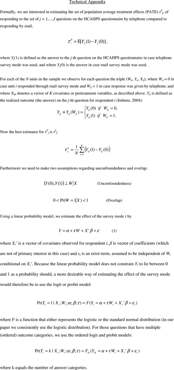
A formal representation is included in the Technical Appendix at the end of this article.
This is also referred to as unconfoundedness, selection on observables or conditional independence.
Imbens (2004) groups these methods into five categories: (a) methods based on estimating the unknown regression functions of the outcome on the covariates; (b) matching on covariates; (c) methods based on the propensity score; (d) combinations of these approaches; and (e) Bayesian methods.
For education, we did not have administrative data, but only data obtained through the survey itself. Education therefore is by definition endogenous (might be subject to a mode effect itself), and for this reason we were hesitant to include it as a covariate. To evaluate the presence of bias resulting from educational differences between mail and phone respondents, we estimate a separate set of models (column b) where education and health status (all obtained from the survey itself) are included as covariates.
We simulated this using the current dataset and found that hospitals could improve one or two places in ranking if they would follow up mail nonrespondents with an additional telephone survey.
REFERENCES
- Acree M, Ekstrand M, Coates TJ, Stall R. Mode Effects in Surveys of Gay Men: A Within-Individual Comparison of Responses by Mail and by Telephone. The Journal of Sex Research. 1999;36(1):67–75. [Google Scholar]
- Brambilla DJ, McKinlay SM. A Comparison of Responses to Mailed Questionnaires and Telephone Interviews in a Mixed Mode Health Survey. American Journal of Epidemiology. 1987;126(5):962–71. doi: 10.1093/oxfordjournals.aje.a114734. [DOI] [PubMed] [Google Scholar]
- Brøgger J, Bakke P, Eide GE, Gulsvik A. Comparison of Telephone and Postal Survey Modes on Respiratory Symptoms and Risk Factors. American Journal of Epidemiology. 2002;155(6):572–6. doi: 10.1093/aje/155.6.572. [DOI] [PubMed] [Google Scholar]
- Burroughs TE, Waterman BM, Cira JC, Desikan R, Claiborne Dunagan W. Patient Satisfaction Measurement Strategies: A Comparison of Phone and Mail Methods. Journal on Quality Improvement. 2001;27(7):349–61. doi: 10.1016/s1070-3241(01)27030-8. [DOI] [PubMed] [Google Scholar]
- Criqui MH, Barrett-Connor E, Austin M. Differences between Respondents and Non-Respondents in a Population-Based Cardiovascular Disease Study. American Journal of Epidemiology. 1978;108(5):367–72. doi: 10.1093/oxfordjournals.aje.a112633. [DOI] [PubMed] [Google Scholar]
- Dillman DA. Mail and Internet Surveys. New York: John Wiley & Sons; 2000. [Google Scholar]
- Elliott MN, Edwards C, Angeles J, Hays Ron D. Patterns of Unit and Item Non-Response in the CAHPS® Hospital Survey. Health Services Research. 2005 doi: 10.1111/j.1475-6773.2005.00476.x. [DOI] [PMC free article] [PubMed] [Google Scholar]
- Fowler FJ, Jr, Gallagher PM, Nederend S. Comparing Telephone and Mail Responses to the CAHPS™ Survey Instrument. Medical Care. 1999;37(3 suppl):MS41–9. doi: 10.1097/00005650-199903001-00005. [DOI] [PubMed] [Google Scholar]
- Fowler FJ, Roman AM, Di ZX. Mode Effects in a Survey of Medicare Prostate Surgery Patients. Public Opinion Quarterly. 1998;62(1):29–46. [Google Scholar]
- Goldstein E, Crofton C, Garfinkel SA, Darby C. Why Another Patient Survey of Hospital Care? Health Services Research. 2005 doi: 10.1111/j.1475-6773.2005.00477.x. http://www.blackwell-synergy.com. [DOI] [PMC free article] [PubMed] [Google Scholar]
- Groves RM, Fowler FJ, Jr, Couper MP, Lepkowski JM, Singer E, Tourangeau R. Survey Methodology. Hoboken, NJ: John Wiley & Sons; 2004. [Google Scholar]
- Hepner KA, Brown JA, Hays RD. Comparison of Mail and Telephone Responses in Assessing Patient Experiences in Receiving Care from Medical Group Practices. Evaluation and the Health Professions. 2005;28(4):1–13. doi: 10.1177/0163278705281074. [DOI] [PubMed] [Google Scholar]
- Hochstim JR. A Critical Comparison of Three Strategies of Collecting Data from Households. Journal of the American Statistical Association. 1967;62(319):976–89. [Google Scholar]
- Imbens GW. Nonparametric Estimation of Average Treatment Effects under Exogeneity: A Review. The Review of Economics and Statistics. 2004;86(1):4–29. [Google Scholar]
- Keller SD, Hepner KA, Hays RD, Zaslavsky AM, O'Malley J, Cleary PD. Psychometric Properties of the HCAHPS Survey. Health Services Research. 2005 doi: 10.1111/j.1475-6773.2005.00471.x. http://www.blackwell-synergy.com. [DOI] [PMC free article] [PubMed] [Google Scholar]
- O'Malley J, Zaslavsky AM, Hays RD, Hepner KA, Keller S, Cleary PD. Exploratory Factor Analyses of the (CAHPS® Hospital) Pilot Survey Responses across and within Medical, Surgical, and Obstetric Service. Health Services Research. 2005 doi: 10.1111/j.1475-6773.2005.00471.x. http://www.blackwell-synergy.com. [DOI] [PMC free article] [PubMed] [Google Scholar]
- Rogers WH. Regression Standard Errors in Clustered Samples. Stata Technical Bulletin. 1993;13:19–23. Reprinted in Stata Technical Bulletin Reprints, vol. 3, 88–94. [Google Scholar]
- Rosenbaum P, Rubin D. The Central Role of the Propensity Score in Observational Studies for Causal Effects. Biometrika. 1983;70(1):41–55. [Google Scholar]
- Rubin DB. Inference and Missing Data. Biometrika. 1976;63:581–92. [Google Scholar]
- Williams RL. A Note on Robust Variance Estimation for Cluster-Correlated Data. Biometrics. 2000;56:645–6. doi: 10.1111/j.0006-341x.2000.00645.x. [DOI] [PubMed] [Google Scholar]
- Wooldridge JM. Econometric Analysis of Cross Section and Panel Data. Cambridge, MA: MIT Press; 2002. [Google Scholar]
Associated Data
This section collects any data citations, data availability statements, or supplementary materials included in this article.
Supplementary Materials