Exploring the Common Dynamics of Homologous Proteins. Application to the Globin Family

Abstract

We present a procedure to explore the global dynamics shared between members of the same protein family. The method allows the comparison of patterns of vibrational motion obtained by Gaussian network model analysis. After the identification of collective coordinates that were conserved during evolution, we quantify the common dynamics within a family. Representative vectors that describe these dynamics are defined using a singular value decomposition approach. As a test case, the globin heme-binding family is considered. The two lowest normal modes are shown to be conserved within this family. Our results encourage the development of models for protein evolution that take into account the conservation of dynamical features.

INTRODUCTION

The connection between molecular structure and biological function is usually restricted to the study of the effects of residues near the active sites in enzymes. However, the overall biological function and its regulation also imply processes like substrate or ligand recognition and diffusion inside the proteins. Fast motions are generally localized, involving only a few atoms that are close to each other, and slow motions typically involve rearrangements of domains and large-scale deformations (1). Correlated motions of residues distant from the active site have been proposed to have an important effect on the rate of catalysis (2). Thus, protein function can involve motions extended over a wide range of timescales from subnanoseconds to several microseconds. Good examples are the phosphoglycerate kinase (3) and hemoglobin (4–6) function's timescales. Furthermore, advances in the development of NMR spectroscopy for studying biomolecular dynamics have provided compelling evidence that, in many cases, conformational dynamics on the microsecond to millisecond timescale governs the rates of biomolecular recognition and catalysis (7–9).

Most amino acids in a protein do not have an obvious direct role in function but create a complex dynamical environment with unusual combination of solid and liquid properties. Indeed, specific paths of energy transfer between distant residues inside a protein are expected to be established in an energy landscape (10,11). The description of collective motions on a global scale (12,13) as well as the identification of dynamical domains inside a protein (14,15) contribute to elucidate the variety of functionalities associated to a given fold.

Protein dynamical properties are of special interest because they establish a link between protein structure and function. Vibrational motions connect different conformations in an energy landscape (16). A protein in a single conformation could not function; motions are an essential link between function and structure.

Nowadays, the great number of available x-ray and NMR protein structures allows a comparative analysis of the dynamic behavior between members of the same fold family. The crystallographic structure is considered as an average structure around which the protein fluctuates and samples different conformations (16,17). The equilibrium dynamics of proteins in the folded state is directly related to their structures. Despite the large number of biological functions that are achieved by a small number of protein structural families, a common dynamics behavior associated with each protein fold might be expected. In that sense, we can attempt to identify the common essential feature of equilibrium dynamics for a given protein fold (18).

We have studied the vibrational dynamics of proteins by normal modes analysis. The low-frequency normal modes describe collective movements that are closely related to the protein's biological function (19). Several studies reveal that simple protein models that use simplified force fields are particularly appropriate to describe the collective motion of proteins (20–23). We used the Gaussian network model (GNM) developed by Bahar et al. (24,25). The model represents a folded protein structure as an elastic network where the α-carbons are chosen as the nodes. Springs connect each node to their neighbors located within a cutoff distance. Previous GNM calculations have shown it as a simple and efficient computational method to study the collective motions of large proteins (25).

The major goal of this work is to develop a general procedure to describe the common dynamics between proteins of the same family. The conservation of protein sequence and structure has been widely studied (26–33). However, conservation of protein dynamics has not been systematically examined yet.

We show how to quantify the similarities between equivalent collective vibrational modes of different proteins using a singular value decomposition (SVD) approach. The SVD method has found wide-ranging applications (34). The related method of principal component analysis, that uses the covariance matrix, was extensively applied to the analysis of extended molecular dynamics simulations (35–38). It has been shown to be useful as a dimensionality reduction technique to transform the original high-dimensional representation of protein motion into a lower-dimensional representation that captures the dominant modes of motion of the protein.

As a test case, we explore the global dynamics of the globin-like family. The globin fold is a good example of divergent evolution (39). It is an all-α fold generally made up of 6–7 helices that provide the scaffold for a well-defined heme-binding pocket (40). Although the three-dimensional (3-D) structure of globins is well preserved, their sequences are very different (41). It is possible to construct templates based on sequence data that can be used to distinguish globins from nonglobins (42). Furthermore, it was possible to identify, from a set of aligned protein structures, a core set of residues that are located at relatively invariant 3-D positions (43). In this work, a new attempt to find a conserved feature for the globins based on their collective dynamics is presented.

METHODS

Normal modes

Calculation with GNM

The vibrational dynamics of a set of homologous proteins are analyzed using the GNM (24,25). The GNM considers the protein as an elastic network. A protein of N residues is represented as a collection of N nodes linked by springs. Every residue undergoes Gaussian fluctuations about its equilibrium position, defined by the coordinates of the α-carbon in the crystallographic structure. This is an isotropic model with N degrees of freedom, each one measuring the amplitude of the fluctuation of one node. No distinction is made between different types of residues, so the springs have a single generic harmonic force constant γ that connects nodes separated by a distance lower than a cutoff value r_c. Thus, the interresidue interaction potential is written as

(1)

where ΔR is the N-dimensional vector whose i^th element is the fluctuation vector ΔR_i of the individual i^th residue, and Γ the N × N Kirchhoff matrix of contacts with elements

(2)

d_ij being the distance between the i^th and j^th residues. The cutoff distance for interactions is taken as 10 Å.

The inverse of the Kirchhoff matrix can be expressed as a product of matrices

(3)

where Q is an orthogonal N × N matrix whose columns u_i are the eigenvectors of Γ, that is, the normal modes, and Λ is the diagonal matrix of eigenvalues λ_i of Γ.

Cross-correlations of fluctuations between the i^th and the j^th residues can be calculated as

(4)

where k_B is the Boltzmann constant, T is the absolute temperature, and the square brackets represent the (ij)^th element of the matrix Γ⁻¹. The temperature factors or B_i-factors, can be expressed in terms of the decomposition of Γ as the sum of contributions from the N-1 internal modes of motion as

(5)

The first eigenvalue of Γ, identically equal to zero, is not included in the summation of Eq. 5. In each case, the value of γ is determined by scaling the theoretical residue fluctuations to best fit the corresponding experimental temperature factors.

Alignment

The normal modes of a protein with N residues are N-dimensional vectors, whose elements are the amplitude of fluctuation of the i^th residue. Thus, normal modes calculated for each of the proteins present different numbers of components. To allow their comparative analysis, they are aligned according to a multiple sequence alignment performed using ClustalX (44). The positions in the alignment that present a gap in any of the considered proteins were neglected. This procedure is consistent with the restriction of “conserved” positions given by Ting et al. (45) to only those positions that are occupied by identical or similar residues in each of the subfamilies. This definition implies that positions occupied by not similar residues even in one subfamily should not be considered as conserved.

Therefore, the dimension of the normal modes is reduced to the number of positions n without gaps in any of the sequences of the alignment. Then, these normal modes with reduced dimension n are normalized.

Reassignment

Normal modes are usually ordered by increasing frequency values. We reassign them according to their dynamical properties, so that each of the m^th modes (m = 1…10) of all the proteins describes similar relative motions. For this purpose, the following procedure is used:

1. A protein-α of reference is considered and the 10 × 10 overlap matrix Q^αβ is calculated with each of the other proteins-β. The elements of Q^αβ are defined as the dot product:

   (6)

   being the i^th element of the r^th normal mode vector of the reference protein-α, and the corresponding element of the s^th normal mode vector of protein-β.

2. Permutations of columns are performed on each of the Q^αβ matrices to maximize the trace.

3. Steps 1 and 2 are repeated considering the different proteins as reference.

The final normal mode assignment is chosen as the one corresponding to the reference protein that had required the least number of permutations in step 2. The normal modes of all the proteins are reassigned according to it.

Representative vectors

Matrices A^m of dimension n × l are built with columns representing the m^th normal mode of each of the l proteins and n being the number of conserved residues in the sequence alignment as described in the Alignment section.

(7)

SVD of each A^m matrix is performed. That is, each A^m is written as the product of an n × l column-orthogonal matrix U^m, an l × l diagonal matrix W^m with positive or zero elements (the singular values), and the transpose of an l × l orthogonal matrix V^m:

(8)

Thus, the elements of matrix A^m can be expressed as the sum of products of columns of U^m and rows of (V^m)^T, with the “weighting factors” being the singular values

(9)

Because of this, in this work, the vector with the highest is considered the representative mode for the m^th normal mode of the matrix A^m.

The family of globins as a test case

We illustrate our approach by comparing the low-frequency collective motions between members of the globin family. The choice of this family as a test case is due to the fact that it is a good example of the way in which natural selection operates on structural changes. Previous work has shown that the relative dispositions of the helices change during the divergent sequence evolution of the family (46). Nevertheless, the consequent large structural changes have had only small effects on the packing of helices involved in positioning the heme group. Thus, globins are a good example of divergent sequence evolution with restricted structure preservation to maintain function.

We used the structural classification of proteins (SCOP) database (47) to select the adequate group of proteins that best represents the fold. We have selected one structure of each of the l = 18 different protein domains belonging to the all-α protein class, globin-like fold, globin-like family (Table 1). For nonmonomeric proteins, only one chain was considered in the alignment. The resulting multiple alignment is represented in Fig. 1.

TABLE 1.

Set of 18 proteins representing the domains of the globin family fold

Protein	Species	PDB code
Hemoglobin I	Clam	1flp
Trematode hemoglobin/myoglobin	Paramphistomum epiclitum	1h97(a)
Glycera globin	Marine bloodworm	2hbg
Myoglobin	Sperm whale	1a6m
Erythrocruorin	Midge, fraction III	1eco
Leghemoglobin	Yellow lupin	2gdm
Nonsymbiotic plant hemoglobin	Rice	1d8u(a)
Hemoglobin	Cartilaginous fish akaei	1cg5(b)
Hemoglobin, β-chain	Mouse	1jeb(b)
Chimeric hemoglobin β-α	Synthetic, based on Homo sapiens sequence	1ch4(a)
Hagfish hemoglobin	Inshore hagfish	1it2(a)
Lamprey globin	Sea lamprey	2lhb
Ascaris hemoglobin, domain 1	Pig roundworm	1ash
Hemoglobin	Innkeeper worm	1ith(a)
Hemoglobin, different isoforms	Sea cucumber	1hlb
Bacterial dimeric hemoglobin	Vitreoscilla stercoraria	1vhb(a)
Flavohemoglobin, N-terminal domain	Alcaligenes eutrophus	1cqx(a)
Dehaloperoxidase	Marine worm	1ewa(a)

For multimeric proteins, only one chain (given in parentheses) was considered in the alignment.

FIGURE 1.

Aligned set of globins. The first column of the blocks displays the PDB code of the proteins and the last column shows the number of residues up to that line. Positions marked with + below the sequences do not present any gap and are retained for our analysis. Protein 1CQX, constituted by 403 residues, is partially shown.

RESULTS AND DISCUSSION

Normal modes and their representative u_r^m vectors

Fig. 2 compares the calculated and experimental temperature factors for hemoglobin I, myoglobin, and lamprey globin. The theoretical values (solid lines) are evaluated from Eq. 5. The experimental data (dashed lines) are the x-ray crystallographic B-factors of the individual α- carbons, reported in the Protein Data Bank (PDB) files of the respective structures (Table 1). The theoretical curves are normalized by suitable choice of the parameter γ. The agreement between theory and experiment is very good. Correlation coefficients of 0.63, 0.60, and 0.70 are obtained for the hemoglobin I (1flp), myoglobin (1a6m), and lamprey globin (2lhb), respectively. Similar results are achieved in calculations performed for the other proteins listed in Table 1. This validates the applicability of the GNM to describe the protein vibrational dynamics of the family.

FIGURE 2.

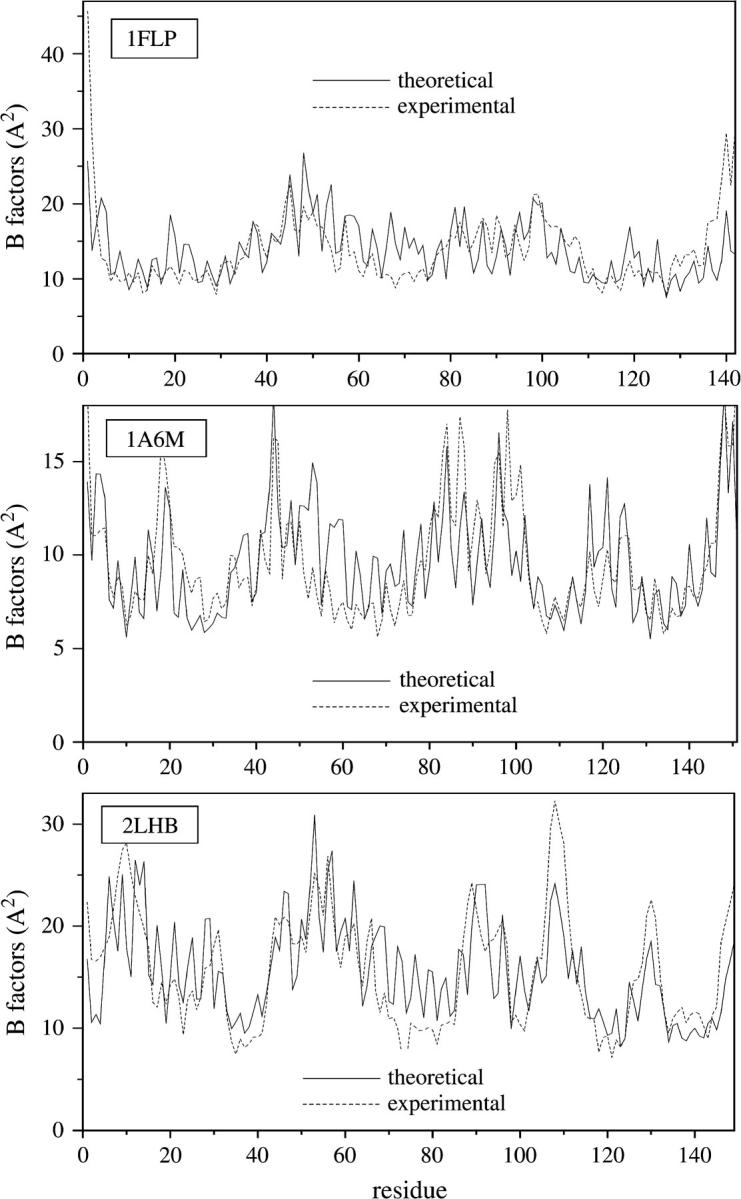
Temperature factors for hemoglobin I (1flp), myoglobin (1a6m), and lamprey globin (2lhb). Solid lines are obtained from Eq. 5, dashed lines from experimental data.

The normal modes were reassigned according to the procedure described in the Reassignment section. The resulting order of modes is shown in Table 2. The reference protein, obtained from the iterative procedure, was the erythrocruorin (1eco). Therefore, the final normal mode assignment was chosen as the one corresponding to this protein. The number of reassignments, with respect to the original order by increasing frequency values, is low for the first two modes. Only the hemoglobin from sea cucumber (1hbl), the α-chain of bacterial dimeric hemoglobin from Vitreoscilla stercoraria (1vhb(a)), and the N-terminal domain of the flavohemoglobin α-chain from Alcaligenes eutrophus (1cqx(a)) have required a reassignment of their two lowest modes. However, the number of reassignments increases significantly for higher frequency normal modes. A greater mode-mixing should be expected when eigenvalues λ_i are close than when they are far apart. This is confirmed in Fig. 3 where the average difference Δl_i between the eigenvalues λ_i and λ_i+1 is displayed as a function of the mode number i before the reassignment. The maximum corresponds to the difference between eigenvalues λ₂ and λ₃. Thus, a relatively large “frequency gap” separates the first two modes from the higher frequency ones. As a result, modes 1 and 2 only rarely are interchanged with higher modes.

TABLE 2.

Reassignment of the modes according to the procedure described in the Reassignment section

Protein PDB code	Normal mode No.
	1	2	3	4	5	6	7	8	9	10
1flp	1	2	3	4	8	6	7	5	10	9
1h97(a)	1	2	3	4	8	10	6	5	9	7
2hbg	1	2	3	4	5	7	6	8	9	10
1a6m	1	2	3	4	6	5	8	7	9	10
1eco	1	2	3	4	5	6	7	8	9	10
2gdm	1	2	4	3	5	10	6	7	8	9
1d8u(a)	1	2	5	4	9	6	7	8	3	10
1cg5(b)	1	2	3	4	8	7	5	6	9	10
1jeb(b)	1	2	6	4	9	7	3	8	5	10
1ch4(a)	1	2	3	4	6	8	7	9	10	5
1it2(a)	1	2	3	4	6	5	8	7	10	9
2lhb	1	2	3	4	5	6	8	7	9	10
1ash	1	2	3	4	5	8	7	6	9	10
1ith(a)	1	2	3	4	5	6	7	8	9	10
1hlb	2	3	5	6	9	7	10	1	4	8
1vhb(a)	2	1	7	4	10	3	6	5	8	9
1cqx(a)	3	2	4	9	10	1	7	8	6	5
1ewa(a)	1	2	3	6	4	5	7	8	9	10

The numbers, located at the reassigned positions, refer to their original order by increasing frequency values.

FIGURE 3.

Average differences between eigenvalues λ_i+1 and λ_i versus mode No. i according to their original order by increasing frequency values before the reassignment.

Fig. 4, a–d, shows the four lowest normal modes for several of the aligned proteins. The solid horizontal lines indicate the zero levels of each curve. Positive values indicate residues moving in the positive direction along the k^th mode (k = 1–4), whereas negative values correspond to residues moving in the opposite direction. The number n of sequentially “conserved” positions, that is, positions without gaps in the alignment, was 99. For these positions we see a common pattern of the collective motion for at least the two lowest normal modes. However, we can see that the conservation between the modes rapidly decays with mode number. The shapes of the representative SVD vectors (m = 1–4) are displayed in Fig. 4, e–h. Only and are good approximations for their corresponding protein normal modes. This is shown in Fig. 4, i–l, where we present the histograms of the relative probability of the dot products (overlaps) Q^α,m

(10)

being the i^th element of the aligned m^th normal mode vector of protein-α, and the corresponding element of the m^th SVD representative vector. The histograms associated with and vectors (Fig. 4, i and j, respectively) show the highest relative probabilities at overlaps >0.9 indicating the important level of conservation of the first and second normal modes within the family. However, the degree of representativity of the vectors decreases for higher values of m.

FIGURE 4.

(a–d) The lowest normal modes (m = 1–4) shapes of 10 aligned proteins from the set of 18; (e–h) the shapes of the corresponding representative SVD vectors (m = 1–4); (i–l) the histograms showing the relative probability of the overlap of aligned normal modes (m = 1–4) with their corresponding representative SVD vector (m = 1–4). Positions with gaps were not included.

The weight of the contribution of each mode to the overall residue fluctuation decreases with its frequency (see Eq. 5). In consequence, the existence of a conserved dynamic behavior at the low-frequency domain is expected to be reflected in a common pattern of the mean-square fluctuations of the α-carbons. This can be seen in Fig. 5 where the temperature factors for several of the aligned proteins are displayed. The average value and standard deviation of the linear correlation coefficients r calculated between all pairs of these patterns is 0.54 ± 0.24. This value was compared with average r values calculated among the squared amplitude shapes of the modes (Table 3). As can be noticed, the B-factors present a degree of correlation similar to those of mode Nos. 1 and 2, despite the relatively low correlation between the higher-frequency modes. Fig. 6 displays the values for the sperm whale myoglobin (1a6m) extending the summation of Eq. 5 to only the first two terms (solid lines) and including all the terms (dotted lines). The global shape of seems to be given by the contribution of the first two terms. Subsequent contributions from higher modes preserve the pattern of the relative amplitudes given by the two lowest-frequency modes. Therefore, a common pattern observed between the two lowest mode shapes of the proteins (Fig. 4) is reflected in a common pattern of the B-factors. On one hand, a common pattern of temperature factors can be related to common patterns of flexibility within the globin fold. On the other hand, a common pattern of the low-frequency normal modes gives us information about a common dynamical correlation between residues, allowing the detection of vibrational energy transfer paths within the family (48).

FIGURE 5.

Superposition of the temperature factors corresponding to eight aligned proteins from the set of 18. Positions with gaps were not included.

TABLE 3.

Averages and standard deviations for the linear correlation coefficients r calculated between the square amplitudes of the modes

Normal mode No.	r
1	0.54 ± 0.26
2	0.59 ± 0.26
3	0.29 ± 0.22
4	0.34 ± 0.24
5	0.27 ± 0.20
6	0.22 ± 0.19
7	0.24 ± 0.17
8	0.18 ± 0.18
9	0.20 ± 0.23
10	0.15 ± 0.14
B-factor	0.54 ± 0.24

FIGURE 6.

Comparison of values for the sperm whale myoglobin (1A6M) extending the summation of Eq. 5 to only the first two terms (solid lines) and all the terms (dotted lines).

A 3-D representation of the first and second normal modes together with their corresponding SVD vectors and is shown for erythrocruorin in Fig. 7. The radius of the bullets are proportional to the amplitudes of motion. Light and dark gray bullets represent 180° out-of-phase movements. That is, the light gray bullets, in accordance to positive values in Fig. 4, a, b, e, and f, indicate the residues moving in the positive direction along the k^th mode, and the dark gray bullets, corresponding to negative values in Fig. 4, a, b, e, and f, refer to the residues moving in the opposite direction. The two lowest modes present low amplitude of motion for helix E residues (positions 35–46 in the alignment; see Fig. 4 e). This helix is in close contact with the heme and makes the dominant contributions to the ligand-binding barrier (49). The coincidence of minima in global mode shapes with ligand-binding roles seems to be a general feature and it was previously pointed out by Keskin et al. (18) in the Rossmann-like fold family. Besides, both and present a large amplitude of motion for helix F (positions 50–61 in the alignment). This result is consistent with NMR spectroscopy experiments that have shown that the F and D helices are the most mobile parts of myoblogin in solution and the last to fold (50,51). Furthermore, helix F is included between the parts with the greatest structural variation (43,52) and consequently less stable parts of the globin fold. Nevertheless, the helix F and loop FG have shown strong dynamic interactions with the heme group (48). Because the pocket between the E and F helices allocates the heme group, Gerstein and co-worker (43) have suggested that the relative motion of the F helix may modulate the environment of the active site allowing the achievement of different oxygen binding affinities among the globins. Thus, a nonconserved structural area like helix F corresponds to a maximum in global mode shapes that can be relevant in the protein functionality.

FIGURE 7.

Three-dimensional representation of the erythrocruorin (1eco). The first and second normal modes and their corresponding SVD vectors and are illustrated. The radius of the bullets are proportional to the amplitudes of motion. Light and dark gray bullets represent 180° out-of-phase movements. The helices and the heme group are also rendered as ribbon.

The patterns of “intrachain” vibrational motions described by and vectors should have also their relevance in the allosteric mechanisms of multimeric proteins. Previous works of Mouawad et al. (53,54) have shown that the T-R transition of the human hemoglobin involves a quaternary rotation of one αβ-dimer with respect to the other followed by an internal tertiary rearrangement within each α- or β-subunit. The latter involves “intrachain” large movements of the C, D, and F helices as well as the so-called “allosteric core” (55,56) (the end of the F helix, the FG corner, and the beginning of the G helix (positions 58–68 in the alignment)). This is in agreement with the regions that display the highest conformational displacements (maxima) in the and modes (Fig. 4, e and f). Therefore, the common collective vibrational motion among the globins, described by the and vectors and responsible for the common patterns of B-factors within the family, fulfill the requirements of relative displacements related either to the mechanism of ligand binding or the tertiary motions that follow the quaternary structure transition in the allosteric mechanism (53,56) proposed for the multimeric members of the family.

Effects of multimerization on the “internal” modes of the individual subunits

The selected group of globins (see Table 1), as representative of the family, includes either monomeric and multimeric members. In the latter cases, a GNM analysis was performed for the overall protein and repeated for individual subunits. Their comparison will allow us to analyze the effect of multimerization on the intrachain motion of the individual subunits.

It is worth noting that the (d-1)^th lowest normal modes of the d-multimers present unique features not observed in the dynamics of the individual subunits. That is, dimers (d = 2) (1h97, 1d8u, 1it2, 1ith, 1vhb, 1cqx, and 1ewa) first lowest normal mode and tetramers (d = 4) (1cg5, 1jeb, and 1ch4) three lowest normal modes involve unique features of relative motions that are not present in the monomer's intrachain dynamics. For instance, the projections of the first five lowest normal modes of the dimeric nonsymbiotic plant hemoglobin (1d8u) in the basis set of the individual subunits normal modes expressed in the whole space of the dimer are 0.30, 0.99, 0.99, 1.00, and 1.00, respectively. Projections of the higher dimers' modes resulted to be ≥0.99 in all cases. In the same way, projections of the tetrameric hemoglobin of mouse (1jeb) in the basis of its corresponding subunit's normal modes are 0.35, 0.44, 0.50, 0.98, and 0.97. As in the other case, projections of the higher tetramers' modes resulted to be ≥0.99 in all cases. Similar results, not shown, were obtained for the others multimers.

The multimer's (d-1)^th lowest modes usually describe relative almost rigid-body movements of the individual subunits about a central hinge region at their interface. In the case of human normal adult hemoglobin, that is composed of four subunits, Xu et al. (57) have shown that the first two lowest modes describe the relative motions of different pairs of the α- and β-subunits. Even more, the authors demonstrate that a GNM analysis can predict the functional conformational transition from the tense (T) form to the relaxed (R) form. This passage was shown to be induced by the slowest global mode of motion of the tetramer. The role that motions at the quaternary structure level have in the allosteric mechanism of this protein was also extensively studied using normal modes analysis (53) and molecular dynamics techniques (54).

This study focuses on the identification and characterization of a unique global dynamics among members of the same family. For this purpose, we have analyzed the conservation of dynamic patterns due to the “intrachain” interactions within monomers or individual subunits of multimers that belong to the globin family. However, it is interesting to consider the extent to which the multimer assembly affects the “internal” modes of the individual subunits.

To address this issue, the squared projections were performed:

(11)

being the i^th element of the r^th normal mode vector of the monomer-α expressed in the whole space of the multimer A, that is, because the dimension n of the subunit's normal mode vectors is smaller than the n × d dimension of the corresponding d-multimer's modes, the former are expanded to n × d dimensions by adding zero coefficients; is the corresponding element of s^th normal mode vector of the corresponding multimer A. For each the highest from each monomer α were summed up:

(12)

being d the number of monomers of the multimer A. The parameter denotes the degree to which the multimer s^th normal mode can be represented by a set of the monomer's normal modes. Leaving out the (d-1)^th lowest multimer's normal modes, that cannot be described by “internal” modes of the individual subunits, the average values of the subsequent 10 lowest modes of each multimer protein are given in Table 4. Thus, the multimer assembly preserves the dynamical properties of the “internal” modes of individual subunits with a high degree of accuracy. Even more, in all dimers, the second lowest mode (s = 2) resulted to be best represented by a linear combination of the first lowest modes (r = 1) of individual subunits. A value of was obtained in all cases. Similarly, the fourth mode of tetramers was best represented by a linear combination of the first subunit's modes.

TABLE 4.

Average values and standard deviations of the 10 lowest normal modes of multimeric proteins

PDB code
1vhb(dimer)	0.87 ± 0.09	0.27	0.99	0.88	0.99	0.83
1cqx(dimer)	0.90 ± 0.09	0.43	0.98	0.83	0.97	0.66
1d8u(dimer)	0.96 ± 0.07	0.21	0.98	0.98	1.00	1.00
1ewa(dimer)	0.97 ± 0.05	0.19	1.00	0.96	1.00	0.99
1h97(dimer)	0.97 ± 0.05	0.11	1.00	0.97	0.99	0.97
1it2(dimer)	0.98 ± 0.03	0.17	1.00	0.97	1.00	0.94
1ith(dimer)	0.94 ± 0.11	0.20	0.99	0.99	0.99	0.94
1jeb(tetramer)	0.84 ± 0.05	0.27	0.31	0.40	0.95	0.83
1cg5(tetramer)	0.90 ± 0.05	0.26	0.31	0.41	0.94	0.87
1ch4(tetramer)	0.83 ± 0.06	0.31	0.36	0.47	0.86	0.69

Quantification of the similarities between equivalent normal modes of the different proteins

Every m^th normal mode (column of matrix A^m) can be spanned by the complete set of l = 18 SVD vectors We reduced the dimensionality of this set to a fraction of the initial dimension, considering subsets of decreasing dimension from the initial 18 SVD vectors. Then, the accuracy of each subset for spanning the m^th normal modes can be calculated as the minimum overlap between every m^th normal mode and its projection on the reduced subset. This can be seen in Fig. 8, where the overlap versus the reduced dimensionality of the subset is displayed for five values of m. Higher order modes do not match as well as the first two modes. For m = 1, <20% of the total dimension of the SVD basis corresponding to A¹ is required to express any of the first normal modes with at least 90% accuracy. The same is observed for the SVD basis associated with A². In contrast, >60% of the SVD basis associated with A¹⁰ is required to express any of the corresponding tenth normal modes at 90% accuracy. Table 5 indicates the number of SVD vectors needed to approximate any of the corresponding normal modes with different degrees of accuracy. The number of required vectors in the subset increases with m. In that way, the reduction of the dimensionality allows us to achieve a quantification of the similarities of collective motions among members of the same family.

FIGURE 8.

The accuracy in the overlap between the m^th normal modes of the globins set and the reduced subset of SVD vectors associated to matrix A^m is plotted for five values of m. For the lowest values of m, a small number of SVD vectors allows the spanning of every normal mode with >90% accuracy.

TABLE 5.

Number of SVD vectors needed to approximate any of the corresponding m^th normal modes of the globins set with at least 90, 70, or 50% accuracy

Normal mode No.	90%	70%	50%
1	3	2	2
2	4	2	1
3	7	4	3
4	7	4	4
5	9	6	4
6	9	6	5
7	8	6	4
8	10	7	5
9	11	8	6
10	11	8	6

CONCLUSION

We have developed a procedure to explore the common dynamics of homologous proteins. The method allows the comparison of patterns of vibrational motions obtained by GNM and involves the alignment, rearrangement, and SVD of the normal modes of homologous proteins. We were able to summarize the common dynamics within a family by the identification of collective coordinates that were conserved during the evolution. This study represents a first step in the proposal of systematic methods and tools to quantify dynamic similarities between homologous proteins and contributes to establish a connection between structure, dynamics, and function.

As a test case, we have considered the globin heme-binding family. We have analyzed the conservation of dynamic patterns due to the “intrachain” interactions within monomers and individual subunits of multimers. The two lowest normal modes have shown to be conserved within the family. A relatively large “frequency gap” separates them from the rest of the modes hindering their mixing. Furthermore, the dynamical properties of these “internal” modes were revealed to be preserved within the assemblies of the oligomeric globins. The differences between the dynamics of the homologous proteins rapidly increase with the average frequency of their corresponding equivalent modes.

The conservation observed in the two lowest modes of the globins was shown to be reflected in the conservation of the B-factors profiles. The conserved patterns are in agreement with the requirements of relative displacement to maintain activity. In this sense, mutations in globins are constrained to produce limited changes (41) at the tertiary level of structure that guarantee a unique pattern of relative flexibilities that provide protein functionalities. New calculations are in progress with different protein fold families.

We show that mutations within a fold family not only conserve a certain degree of protein structure but also features of their dynamics. We have recently developed successful models that take into consideration the effect of structure conservation on sequence divergence (58–60). These results encourage the development of theoretical methods for protein evolution based on the conservation of dynamical features. The representative vectors can be considered as candidates for this purpose.

References

- 1.Hinsen, K. A., and G. R. Kneller. 2000. Projection methods for the analysis of complex motions in macromolecules. Mol. Sim. 23:275–292. [Google Scholar]
- 2.Doruker, P., A. R. Atilgan, and I. Bahar. 2000. Dynamics of proteins predicted by molecular dynamics simulations and analytical approaches: application to α-amylase inhibitor. Proteins. 40:512–524. [PubMed] [Google Scholar]
- 3.Mouawad, L., M. Desmadril, D. Perahia, J. M. Yon, and J. C. Brochon. 1990. The effects of ligands on the conformation of phosphoglycerate kinase: fluorescence anisotropy decay and theoretical interpretation. Biopolymers. 30:1151–1160. [DOI] [PubMed] [Google Scholar]
- 4.Kiger, L., C. Poyart, and M. C. Marden. 1993. Oxygen and CO binding to triply NO and asymmetric NO/CO hemoglobin hybrids. Biophys. J. 65:1050–1058. [DOI] [PMC free article] [PubMed] [Google Scholar]
- 5.Hofrichter, J., E. R. Henry, A. Szabo, L. P. Murray, A. Ansari, C. M. Jones, M. Coletta, G. Falcioni, M. Brunoni, and W. A. Eaton. 1991. Dynamics of the quaternary conformational change in trout hemoglobin. Biochemistry. 30:6583–6598. [DOI] [PubMed] [Google Scholar]
- 6.Jayaraman, V., K. R. Rodgers, I. Mukerji, and T. G. Spiro. 1995. Hemoglobin allostery: resonance Raman spectroscopy of kinetic intermediates. Science. 269:1843–1848. [DOI] [PubMed] [Google Scholar]
- 7.Feher, V. A., and J. Cavanagh. 1999. Millisecond-timescale motions contribute to the function of the bacterial response regulator protein Spo0F. Nature. 400:289–293. [DOI] [PubMed] [Google Scholar]
- 8.Stock, A. 1999. Relating dynamics to function. Nature. 400:221–222. [DOI] [PubMed] [Google Scholar]
- 9.Akke, M. 2002. NMR methods for characterizing microsecond to millisecond dynamics on recognition and catalysis. Curr. Opin. Struct. Biol. 12:642–647. [DOI] [PubMed] [Google Scholar]
- 10.Frauenfelder, H., B. H. McMahon, and P. W. Fenimore. 2003. Myoglobin: the hydrogen atom of biology and a paradigm of complexity. Proc. Natl. Acad. Sci. USA. 100:8615–8617. [DOI] [PMC free article] [PubMed] [Google Scholar]
- 11.Bourgeois, D., B. Vallone, F. Schotte, A. Arcovito, A. E. Miele, G. Sciara, M. Wulff, P. Anfinrud, and M. Brunori. 2003. Complex landscape of protein structural dynamics unveiled by nanosecond Laue crystallography. Proc. Natl. Acad. Sci. USA. 100:8704–8709. [DOI] [PMC free article] [PubMed] [Google Scholar]
- 12.Hayward, S., and N. Go. 1995. Collective variable description of native protein dynamics. Annu. Rev. Phys. Chem. 46:223–250. [DOI] [PubMed] [Google Scholar]
- 13.Kitao, A., and N. Go. 1999. Investigating protein dynamics in collective coordinate space. Curr. Opin. Struct. Biol. 9:164–169. [DOI] [PubMed] [Google Scholar]
- 14.Hinsen, K. A. 1998. Analysis of domain motions by approximate normal mode calculations. Proteins. 33:417–429. [DOI] [PubMed] [Google Scholar]
- 15.Hinsen, K., A. Thomas, and M. J. Field. 1999. Analysis of domain motions in large proteins. Proteins. 34:369–382. [PubMed] [Google Scholar]
- 16.Frauenfelder, H., S. G. Sligar, and P. G. Wolynes. 1991. The energy landscape and motions of proteins. Science. 254:1598–1603. [DOI] [PubMed] [Google Scholar]
- 17.Elber, R., and M. Karplus. 1987. Multiple conformational states of proteins: a molecular dynamics analysis of myoglobin. Science. 235:318–321. [DOI] [PubMed] [Google Scholar]
- 18.Keskin, O., R. L. Jernigan, and I. Bahar. 2000. Proteins with similar architecture exhibit similar large-scale dynamic behavior. Biophys. J. 78:2093–2106. [DOI] [PMC free article] [PubMed] [Google Scholar]
- 19.Berendsen, J. C., and S. Hayward. 2000. Collective protein dynamics in relation to function. Curr. Opin. Struct. Biol. 10:165–169. [DOI] [PubMed] [Google Scholar]
- 20.Tirion, M. M. 1996. Large amplitude elastic motions in proteins from a single-parameter, atomic analysis. Phys. Rev. Lett. 77:1905–1908. [DOI] [PubMed] [Google Scholar]
- 21.Bahar, I., B. Erman, R. L. Jernigan, A. R. Atilgan, and D. G. Covell. 1999. Collective motions in HIV-1 reverse transcriptase: examination of flexibility and enzyme function. J. Mol. Biol. 285:1023–1037. [DOI] [PubMed] [Google Scholar]
- 22.Bahar, I., and R. L. Jernigan. 1999. Cooperative fluctuations and subunit communication in tryptophan synthase. Biochemistry. 38:3478–3490. [DOI] [PubMed] [Google Scholar]
- 23.Hinsen, K., and G. R. Kneller. 1999. A simplified force field for describing vibrational protein dynamics over the whole frequency range. J. Chem. Phys. 24:10766–10769. [Google Scholar]
- 24.Haliloglu, T., I. Bahar, and B. Erman. 1997. Gaussian dynamics of folded proteins. Phys. Rev. Lett. 79:3090–3093. [Google Scholar]
- 25.Bahar, I., A. R. Atilgan, and B. Erman. 1997. Direct evaluation of thermal fluctuations in proteins using a single-parameter harmonic potential. Fold. Des. 2:173–181. [DOI] [PubMed] [Google Scholar]
- 26.Levitt, M., and C. Chothia. 1976. Structural patterns in globular proteins. Nature. 261:552–558. [DOI] [PubMed] [Google Scholar]
- 27.Ptitsyn, O. B., and A. V. Finkelstein. 1981. Similarities in protein topologies: evolutionary divergence, functional convergence or principles of folding. Q. Rev. Biophys. 13:339–386. [DOI] [PubMed] [Google Scholar]
- 28.Chothia, C. 1984. Principles that determine the structure of proteins. Annu. Rev. Biochem. 53:537–572. [DOI] [PubMed] [Google Scholar]
- 29.Chothia, C., and A. M. Lesk. 1986. The relation between the divergence of sequence and structure in proteins. EMBO J. 5:823–826. [DOI] [PMC free article] [PubMed] [Google Scholar]
- 30.Orengo, C. A., T. P. Flores, W. R. Taylor, and J. M. Thornton. 1993. Identifying and classifying protein fold families. Protein Eng. 6:485–500. [DOI] [PubMed] [Google Scholar]
- 31.Orengo, C. A., D. T. Jones, and J. M. Thornton. 1994. Protein superfamilies and domain superfolds. Nature. 372. 6507: 631–634. [DOI] [PubMed] [Google Scholar]
- 32.Wood, T. C., and W. R. Pearson. 1999. Evolution of protein sequences and structures. J. Mol. Biol. 291:977–995. [DOI] [PubMed] [Google Scholar]
- 33.Koehl, P. 2001. Protein structure similarities. Curr. Opin. Struct. Biol. 11:348–353. [DOI] [PubMed] [Google Scholar]
- 34.Wall, M. E., A. Rechtsteinner, and L. M. Rocha. 2003. Singular value decomposition and principal component analysis. In A Practical Approach to Microarray Data Analysis. D. P. Berrar, W. Dubitzky, and M. Granzow, editors. Kluwer, Norwell, MA. 91–109.
- 35.Ichiye, T., and M. Karplus. 1991. Collective motions in proteins: a covariance analysis of atomic fluctuations in molecular dynamics and normal mode simulations. Proteins. 11:205–217. [DOI] [PubMed] [Google Scholar]
- 36.Amadei, A., A. B. M. Linssen, and H. J. C. Berendsen. 1993. Essential dynamics of proteins. Proteins. 17:412–425. [DOI] [PubMed] [Google Scholar]
- 37.Balsera, M. A., W. Wriggers, Y. Oono, and K. Schulten. 1996. Principal component analysis and long time protein dynamics. J. Phys. Chem. 100:2567–2572. [Google Scholar]
- 38.Hayward, S., A. Kitao, and N. Go. 1994. Harmonic and anharmonic aspects in the dynamics of BPTI: a normal mode analysis and principal component analysis. Protein Sci. 3:936–943. [DOI] [PMC free article] [PubMed] [Google Scholar]
- 39.Monees, L., J. Vanfleteren, Y. Van de Peer, K. Peeters, O. H. Kapp, J. Czeluzniak, M. Goodman, M. Blaxter, and S. N. Vinogradov. 1996. Globins in nonvertebrate species: dispersal by horizontal gene transfer and evolution of the structure function relationships. Mol. Biol. Evol. 13:324–333. [DOI] [PubMed] [Google Scholar]
- 40.Aronson, H. E., W. E. Royer, and W. A. Hendrickson. 1994. Quantification of tertiary structural conservation despite primary sequence drift in the globin fold. Protein Sci. 3:1706–1711. [DOI] [PMC free article] [PubMed] [Google Scholar]
- 41.Lesk, A. M., and C. Chothia. 1980. How different amino acid sequences determine similar protein structures: the structure and evolutionary dynamics of the globins. J. Mol. Biol. 136:225–270. [DOI] [PubMed] [Google Scholar]
- 42.Bashford, D., C. Chothia, and A. M. Lesk. 1987. Determinants of a protein fold. Unique features of the globin amino acid sequences. J. Mol. Biol. 196:199–216. [DOI] [PubMed] [Google Scholar]
- 43.Altman, R. B., and M. B. Gerstein. 1994. Finding an average core structure: application to the globins. 1994. Proceedings of the Second International Conference on Intelligent Systems for Molecular Biology. AAAI Press, Menlo Park, CA. 19–27. [PubMed]
- 44.Thompson, J. D., T. J. Gibson, F. Plewniak, F. Jeanmougin, and D. G. Higgins. 1997. The ClustalX windows interface: flexible strategies for multiple sequence alignment aided by quality analysis tools. Nucleic Acids Res. 24:4876–4882. [DOI] [PMC free article] [PubMed] [Google Scholar]
- 45.Ptitsyn, O. B., and K. H. Ting. 1999. Non-functional conserved residues in globins and their possible role as a folding nucleus. J. Mol. Biol. 291:671–682. [DOI] [PubMed] [Google Scholar]
- 46.Chothia, C., and A. M. Lesk. 1987. The evolution of protein structures. Cold Spring Harbor Symp. Quant. Biol. 52:399–405. [DOI] [PubMed] [Google Scholar]
- 47.Murzin, A. G., S. E. Brenner, T. Hubbard, and C. Chothia. 1995. SCOP: a structural classification of proteins database for the investigation of sequences and structures. J. Mol. Biol. 247:536–540. [DOI] [PubMed] [Google Scholar]
- 48.Seno, Y., and N. Go. 1990. Deoxymyoglobin studied by the conformational normal mode analysis. J. Mol. Biol. 216:95–109. [DOI] [PubMed] [Google Scholar]
- 49.Case, D. A., and M. Karplus. 1979. Dynamics of ligand binding to heme proteins. J. Mol. Biol. 132:343–368. [DOI] [PubMed] [Google Scholar]
- 50.Cocco, M. J., and J. T. J. Lecomte. 1990. Characterization of hydrophobic cores in apomyoglobin: a proton NMR spectroscopy study. Biochemistry. 29:11067–11072. [DOI] [PubMed] [Google Scholar]
- 51.Jennings, P. A., and P. E. Wright. 1993. Formation of molten globule intermediate early in the kinetic folding pathway of apomyoglobin. Science. 262:892–896. [DOI] [PubMed] [Google Scholar]
- 52.Baldwin, J., and C. Chothia. 1979. Haemoglobin: the structural changes related to ligand binding and its allosteric mechanism. J. Mol. Biol. 129:175–220. [DOI] [PubMed] [Google Scholar]
- 53.Mouawad, L., and D. Perahia. 1996. Motions in hemoglobin studied by normal mode analysis and energy minimization: evidence for the existence of tertiary T-like, quaternary R-like intermediate structures. J. Mol. Biol. 258:393–410. [DOI] [PubMed] [Google Scholar]
- 54.Mouawad, L., D. Perahia, C. H. Robert, and C. Guilbert. 2002. New insights into the allosteric mechanism of human hemoglobin from molecular dynamics simulations. Biophys. J. 82:3224–3245. [DOI] [PMC free article] [PubMed] [Google Scholar]
- 55.Gelin, B. R., A. W. M. Lee, and M. Karplus. 1983. Hemoglobin tertiary structural change on ligand binding: its role on the co-operative mechanism. J. Mol. Biol. 171:489–559. [DOI] [PubMed] [Google Scholar]
- 56.Borgstahl, G. E. O., P. H. Rogers, and A. Arnone. 1994. The 1.9 Å Structure of deoxyβ4 hemoglobin. Analysis of the partitioning of quaternary-associated and ligand-induced changes in tertiary structure. J. Mol. Biol. 236:831–843. [DOI] [PubMed] [Google Scholar]
- 57.Xu, C., D. Tobi, and I. Bahar. 2003. Allosteric changes in protein structure computed by a simple mechanical model: hemoglobin T ↔ R2 transition. J. Mol. Biol. 333:153–168. [DOI] [PubMed] [Google Scholar]
- 58.Parisi, G., and J. Echave. 2001. Structural constraints and emergence of sequence patterns in protein evolution. Mol. Biol. Evol. 18:750–756. [DOI] [PubMed] [Google Scholar]
- 59.Parisi, G., and J. Echave. 2004. The structurally constrained protein evolution model accounts for sequence patterns of the LβH superfamily. BMC Evol. Biol. 4:41. [DOI] [PMC free article] [PubMed] [Google Scholar]
- 60.Fornasari, M. S., G. Parisi, and J. Echave. 2002. Site-specific amino-acid replacement matrices from structurally constrained protein evolution simulations. Mol. Biol. Evol. 19:352–356. [DOI] [PubMed] [Google Scholar]