Sedimentation Velocity Analysis of Heterogeneous Protein-Protein Interactions: Lamm Equation Modeling and Sedimentation Coefficient Distributions c(s)

Abstract

We describe algorithms for solving the Lamm equations for the reaction-diffusion-sedimentation process in analytical ultracentrifugation, and examine the potential and limitations for fitting experimental data. The theoretical limiting case of a small, uniformly distributed ligand rapidly reacting with a larger protein in a “constant bath” of the ligand is recapitulated, which predicts the reaction boundary to sediment with a single sedimentation and diffusion coefficient. As a consequence, it is possible to express the sedimentation profiles of reacting systems as c(s) distribution of noninteracting Lamm equation solutions, deconvoluting the effects of diffusion. For rapid reactions, the results are quantitatively consistent with the “constant bath” approximation, showing c(s) peaks at concentration-dependent positions. For slower reactions, the deconvolution of diffusion is still partially successful, with c(s) resolving peaks that reflect the populations of sedimenting species. The transition between c(s) peaks describing reaction boundaries of moderately strong interactions (K_D ∼ 10⁻⁶ M) or resolving sedimenting species was found to occur in a narrow range of dissociation rate constant between 10⁻³ and 10⁻⁴ s⁻¹. The integration of the c(s) peaks can lead to isotherms of species populations or s-value of the reaction boundary, respectively, which can be used for the determination of the equilibrium binding constant.

INTRODUCTION

The hydrodynamic separation of protein species after application of a high gravitational force is a powerful tool in the study of macromolecules, which provides unique information for the study of both synthetic and biological macromolecules in solution (1). The dynamics of the sedimentation process allows the detection of the sedimenting species or components and their interactions with high sensitivity, and the characterization by first-principle-based analysis. When studying protein-protein interactions, sedimentation techniques allow distinguishing multiple sedimenting species in free solution while maintaining reversibly formed complexes in a bath of their components at all times. This permits the study of self-association as well as heterogeneous protein interactions. In particular, the hydrodynamic resolution of sedimentation velocity can be advantageous for the characterization of extended mixed self- and heteroassociations of two or more proteins. The introduction of modern computational approaches in the last decades has enabled significant further development of ultracentrifugation analysis. In particular, it had a large impact on sedimentation velocity because it allowed the routine use in the data analysis of the Lamm equation (2), the partial-differential equation describing the time course of sedimentation (for example, see (3–11); for general reviews, see, for example, (12–17); a recent introduction and protocol for the practical application can be found in (18)).

The analysis of protein interactions by sedimentation velocity requires unraveling sedimentation, diffusion, and chemical reaction processes that take place during the experiment. So far, no general method is known that would reveal both the number of sedimenting species and their mutual interactions. Instead, two separate approaches exist for: 1), determining the number of species, based on sedimentation equations for distributions of noninteracting macromolecules, and 2), for the data analysis incorporating chemical reactions assuming specific models. A hybrid approach was recently developed to reveal the number and composition of sedimenting complexes for heterogeneous associations from multisignal analysis (19), assuming reactions to be slow on the timescale of sedimentation.

The first approach consists of a family of methods for calculating sedimentation coefficient distributions, obtained through extrapolation (the van Holde-Weischet method (20,21)), transformation of a data subset (the dc/dt approach to g(s*) (22)), or least-squares boundary modeling procedures (ls-g*(s) (23), c(s) (24), and c_k(s) (19)). They differ in the extent to which diffusion can be deconvoluted from the sedimentation coefficient distributions, ranging from no corrections (in g(s*) and ls-g*(s)), corrections for single species or clearly separating sedimentation boundaries (in the van Holde-Weischet method), to the approximate deconvolution for all species using hydrodynamic scaling laws and a single weight-average frictional ratio (c(s) and c_k(s)). Of particular interest for this article is the c(s) method, as the deconvolution of diffusion and sedimentation is achieved through a detailed analysis of the sedimentation velocity boundary shapes, leading to a very high hydrodynamic resolution.

All sedimentation coefficient distributions have the advantage that no prior knowledge on the number of sedimenting species or their mode of interaction is required. Because they are based on equations for noninteracting species, however, they will exhibit specific characteristic features if chemical reactions on the timescale of sedimentation modulate the evolution of concentration profiles in the experiment. For example, in the presence of fast reactions, all the differential sedimentation coefficient distributions g(s*), ls-g*(s), c(s), and c_k(s) will exhibit peaks at positions that do not necessarily reflect the sedimentation coefficient of the molecular species, but are governed instead by chemical interconversion of the species as described in theory by Gilbert and Jenkins (25,26). This can be diagnosed best in series of experiments at different concentrations of the protein mixture. In this article, we examine these characteristic features of c(s) in the presence of chemical reactions on different timescales.

The second approach for the analysis, explicitly modeling the chemical reactions, can be taken once a model for the species and their interactions has been established or hypothesized. As is well known, the differential sedimentation coefficient distributions can be integrated to give weight-average sedimentation coefficients, and the isotherms resulting from experiments at different loading composition can be fitted with different interaction models (27). Although very powerful, this technique extracts only thermodynamic information from the different populations of species at different loading concentrations. A more comprehensive approach is to model the sedimentation velocity data directly with the partial differential equation for the sedimentation/diffusion/reaction process, which is a system of coupled Lamm equations (28). This approach was developed by Cann and Goad (29), Cox (6), Claverie (30), and others, and related algorithms are currently implemented for the modeling of experimental data in software programs including BPCFIT (5,8), SEDANAL (11), and SEDFIT and SEDPHAT (9,31). This article describes new algorithms for solving the Lamm equation for reacting systems, and provides examples for the direct global modeling of sedimentation velocity data obtained at different loading composition and detection signals. An important question to be explored is the limit of information that can be extracted from experimental sedimentation velocity data.

The hypothetical ideal case of the sedimentation of a large component in a constant bath of a fast reacting small ligand was introduced previously by Krauss et al. (32) and Urbanke and colleagues et al. (33,34). The sedimentation/diffusion/reaction equations of this theoretical limiting case can be analytically solved and one arrives at characteristic sedimentation and diffusion coefficients of the sedimenting system. This can be exploited for the thermodynamic analysis of the binding isotherm (32), which is alternate to and may in some cases be more advantageous than the study of weight-average s-values. The limits of validity of this ideal model for interactions of dissimilar-sized proteins are analyzed with the help of numerical Lamm equation solutions. This special case can also provide a useful background for understanding the characteristic features of c(s) for fast reactive systems, which will be further explored in the accompanying article (35) on the comparison of c(s) distributions with the asymptotic boundary shapes predicted by Gilbert-Jenkins theory (26).

THEORY

The Lamm equation for a system of reacting components can be written as

(1)

where c_k(r,t) denotes the concentration of solute k at radius r and time t, J_k,tr denotes the transport flux of solute k, ω denotes the angular velocity of the rotor, s_k and D_k denote the sedimentation and diffusion coefficients of the solute, and q_k denote the local chemical reaction rates, respectively (36).

Sedimentation in a constant bath of ligand

The following recapitulates the theory described earlier by Krauss et al. (32) and Urbanke and colleagues (33,34). We consider a system of two components A and B that react and come to an instantaneous equilibrium with a complex, denoted C. The evolution of the system is given by

(2)

where a, b, and c denote the local species concentrations and q the reaction fluxes, respectively, which obey mass conservation and mass action law

(3)

Guided by the assumption that A is very small such that it sediments much slower and high diffusion would rapidly diminish any concentration gradients, we examine the case in which B and C are in a region of negligible concentration gradient of free A for all times. Although strictly this situation would be difficult to realize for infinitely fast interactions, it is a highly interesting limiting case. (The relationships of this model with Gilbert-Jenkins theory will be discussed below.) With , from mass action law Eq. 3 follows that the spatial derivatives of B and C are proportional, . In the hypothetical region of constant A, the migrating species are B and C, and their evolution is

(4)

If we sum over the concentration of the migrating species B and C, denoted as , we find and, because the reaction fluxes cancel, we obtain the conventional Lamm equation of a single noninteracting species

(5)

with weight-average diffusion and sedimentation coefficients

(6)

Therefore, we conclude that where the concentration gradient of the smaller species A is negligible, the species B and the complex C sediment jointly like a single ideal species. In this limiting case, the system has two characteristic sedimentation and diffusion coefficients, which should be visible in a slower boundary migrating with s and D of component A, and a faster boundary migrating in the plateau region of free A with s and D following the weight average of B and C. It can be shown that this holds true also more generally for interactions with multiple binding sites of A on B (33,34). Using finite element solutions of the system of Lamm equations we will study under which conditions this is a realistic limiting case (see below). In particular, we deviate from the original assumption of a small ligand, to test the predictions of this limiting case for interactions between moderately large proteins.

Finite element solution

The discretization of Eq. 1 can be based on the elements

(7)

with an underlying grid of radial points r₁…r_N that may be equidistant and constant in time (30), or logarithmically spaced grid with a time dependence like sedimenting point particles (9). The grid starts at the meniscus (r₁ = m) and ends at the bottom (r_N = b) of the solution column. For simplicity, a static grid will be assumed in the following. The first step to obtain a matrix equation for the propagation is the multiplication of Eq. 1 with all elements P_i and integration in radial coordinates

(8)

Integration by parts of the right-hand side leads to

(9)

where it was used that the sedimentation fluxes J disappear at the beginning and end of the solution column (30) (see below). With the approximations and analogous , we arrive at a matrix equation

(10)

with the standard tridiagonal matrices A⁽¹⁾, A⁽²⁾, and B from pairwise integrals of the elements P_i (6,9,30). Modifications can be applied for semiinfinite solution columns (see below). With the vector notation and for the concentration and reaction flux coefficients of species k, this can be simplified to

(11)

The evolution in time is calculated by separately evaluating both terms of Eq. 11, corresponding to sequential spatial migration and chemical reaction fluxes. This separation was introduced previously in the numerical simulation of transport processes of reacting systems (as reviewed by Cox and Dale (6)).

Because very large concentration gradients may be generated during the simulation, it is important to carefully consider the time steps and the propagation scheme to ensure precision and avoid numerical instabilities. For nonreacting systems, we have introduced previously an adaptive time increment and applied the second-order Crank-Nicholson scheme (37), in which the propagation is not based on the coefficients in the beginning of the time step, but on the average during the step (38). This is applied to calculate an estimated spatial propagation (denoted ) from time t₁ to time t₂, according to

(12)

(with ), which can be used to generate an initial estimate of the concentration change caused by the chemical conversion during this time step (see below), leading to a new predicted concentration

(13)

At this point, a correction can be applied that takes into account that the reaction takes place during the time step and already contributes to sedimentation,

(14)

which can be used, in turn, for a better prediction of the reaction rates .

For the numerical evaluation of the chemical reaction, different approaches were taken dependent on the model of an instantaneous equilibrium (for reactions much faster than the timescale of sedimentation), or that of intermediate, finite reaction kinetics. For instantaneous equilibria, at each radius the concentration was completely relaxed to the equilibrium concentrations for given local composition

(15)

where was calculated based on the laws of mass action and mass conservation. (The resulting nonlinear equation system can be solved very efficiently using the Van Wijngaarden-Dekker-Brent root-finding algorithm (38), taking advantage of the continuity of the component concentrations for neighboring radial points, and in combination with analytical expressions for limiting cases of the interaction isotherm.) For finite reaction kinetics, the concentration change was calculated directly from a linear approximation of the rate equations. The linear approximation of the rate equations seems satisfactory, as any requirement for higher precision would indicate an incompatibility with the precision of the predicted spatial migration, in particular in the absence of a corrector step Eq. 14. However, to ensure that this does not introduce significant errors, the time step Δt was limited so that at each radius the fractional change in concentration from both sedimentation and reaction does not exceed

(16)

at all radii for which is above a threshold value. As a result, for fast reactions the reaction itself is limiting the numerical step size, and for slow reactions the sedimentation is limiting. This algorithm was implemented for a static grid, for conventional finite and semiinfinite solution columns (see below), and with and without the correction steps of Eqs. 13 and 14 .

A numerical integration of the Lamm equation with chemical reactions using the Euler method of discretization has been developed by one of us (C.U.) before (5) and is available in the program BPCFIT (8). We simulated the case of an A + B = C system with K_D = 10⁻⁷M, k_off =5 10⁻⁴ s⁻¹, 0.2 μM B and 0.5 μM A as loading concentrations and sedimentation constants S_A = 6 S, S_B = 9 S, and S_C = 12 S. Both BPCFIT and SEDPHAT based on the algorithm described above yielded virtually indistinguishable time-dependent concentration profiles, thus proving the correct implementation of the algorithms.

Solving the Lamm equation for a semiinfinite cell

In the finite element solution above, it was used that the transport fluxes disappear at the beginning and end of the solution column. In more detail, integration by parts of Eq. 8 leads to

(17)

where conventionally the boundary conditions are used that the ends of the solution column are impermeable to the solute, i.e., at all times (30). A numerically more favorable Lamm equation solution is possible for a permeable wall at the bottom of the solution column (). This is equivalent to the limiting case of a solution column that does not possess a bottom and extends to infinity (but it starts and behaves as usual at the meniscus). Physically, this provides a correct description of the macromolecular behavior for those regions of the solution column that are not affected by back-diffusion from the bottom. This region can be easily discerned from visual inspection of the experimental sedimentation data, and for species of high molar mass at high angular velocity—a situation typical for sedimentation velocity experiments of proteins >10 kDa—the region unaffected by back-diffusion comprises most of the data. In fact, the region of back-diffusion is routinely excluded from the data analysis because of the difficulty of reliable data acquisition and modeling in the steep concentration gradients close to the bottom, and because of possible pelleting of the material. As a consequence, it can be very useful to avoid the most time-consuming and potentially instable numerical computation of the accumulation at the bottom by using the boundary condition of a permeable bottom.

For a permeable bottom, Eq. 17 shows that extra terms only occur for row N, because from Eq. 7 it can be seen that for and . After discretization of c(r,t) as linear combination of the elements P_k, and evaluation of the extra flux term by Eq. 1, we find

(18)

It follows that the permeable bottom can be implemented by simple modification of three elements of the sedimentation and diffusion matrices

(19)

By eliminating the steep concentration gradients at the bottom of the cell, the numerical solution of the Lamm equation with chemical reaction is considerably more stable and efficient.

The sedimentation coefficient distribution c(s) of noninteracting diffusing species

In this section, we briefly recapitulate the model of a differential distribution of noninteracting diffusing species (24). The signal a(r,t) from the sedimentation process of an unknown mixture is approximated as a superposition

(20)

where c(s) denotes the differential sedimentation coefficient distribution in units of the observed signal. χ₁(s,F,r,t) denotes the solution of the Lamm Eq. 1 in the absence of a reaction, at unit concentration and with sedimentation coefficient s and a hydrodynamic frictional ratio F = (f/f₀) that scales the diffusion coefficients to the sedimentation coefficients according to

(21)

(with η and ρ the solvent viscosity and density, respectively, and the partial-specific volume of the macromolecules). Exploiting that the frictional ratio is not a strongly shape-dependent quantity, F is approximated by a constant weight average value F_w for the complete distribution, where the value of F_w is adjusted during least-squares fit of Eq. 20 (39). In most cases, the c(s) distribution is calculated using maximum entropy regularization (40), which results in the most parsimonious distribution c(s) that fits that data with a quality statistically indistinguishable from the overall best fit, and using algebraic elimination of the typical time-invariant and radial-invariant noise components (41,42).

Recently, an extension to multicomponent sedimentation coefficient distributions c_k(s) was introduced, which can be calculated from globally modeling multiple signals λ acquired during the sedimentation process

(22)

provided that each component k contributes in a characteristic way to the signal λ according to a predetermined extinction coefficient (or molar signal increment) matrix ɛ_kλ (19). It is assumed that the signal increments are constant, implying the absence of hyper and hypochromicity, which can be independently verified in a spectrophotometer. The number of signals Λ in current commercial instrumentation is up to four, which in theory could be used to distinguish the same number of spectrally different protein components K; c_k(s) reflects the sedimentation coefficient distribution of each component in molar units, and as shown by Balbo et al. (19), this can permit the determination of the stoichiometry of protein complexes.

RESULTS

Modeling sedimentation profiles of reacting systems with Lamm equations

The finite element algorithms were implemented for instantaneous and finite kinetics for heterogeneous association models with a single site and two sites, and for several single-step and two-step self-association models. Because there are no general analytical solutions to the sedimenting reaction/diffusion system, it is important to study the accuracy of the simulation for known special cases. We tested the precision by several known criteria: i), mass conservation was obeyed at all times separately for both components; ii), the limiting case of noninteracting species was correctly approached for c_A ≪ K_D, c_A ≫ K_D, and k_off < 10⁻⁶/s; iii), with sedimentation parameters of A and B identical, the rapid equilibrium model was equivalent to an instantaneous single-component self-association model computed with concentration-dependent sedimentation and diffusion coefficients (43) (after consideration of statistical factors); iv), with sedimentation parameters of A and B identical, the kinetic heteroassociation models gave results consistent with the kinetic self-association models; v), models with fast reaction kinetics calculated via rate equations approached the same distributions as those from models calculated with instantaneous local chemical equilibrium using mass action law (for example, for species with s-values of 7 and 10 S sedimenting at 50,000 rpm, this limit was attained for k_off > 0.03/s); vi), sedimentation equilibrium distributions consistent with thermodynamic analytical solution were obtained; vii), the isotherm of weight-average sedimentation coefficients (from the analysis of sedimentation data by integration of the c(s) distribution (31)) was consistent with binding constants and s-values; and viii), the two-site models in case of strong negative cooperativity approached the single-site models (considering statistical factors). Using realistic parameters for average-sized proteins, the root-mean-square (rms) errors in these cases were found to be in the order of 10⁻³ or better, which is below the experimental error of data acquisition. ix), For the special case of instantaneous reactions of species in the limit of very small diffusion coefficients, the boundary profiles were consistent with those predicted by Gilbert-Jenkins theory (35,26 ). x), Finally, for conditions of partially reaction-controlled sedimentation of dissimilar-sized proteins, for which no special case or approximate solution exists, the predicted profiles from SEDPHAT were compared to those obtained with the independently implemented software BPCFIT (8). Excellent agreement was observed, supporting the correctness of the Lamm equation solution. We observed limitations in the numerical stability of the approach described here for cases where the component concentrations were significantly higher than the equilibrium dissociation constant, a case that can be adequately modeled with populations of noninteracting species. Further, numerical oscillations and error amplification were encountered for cases where very steep concentration gradients were generated. This was not always improved using the predictor-corrector scheme of Eqs. 14 and 15. However, this problem was absent when using the model for the spatial propagation in a semiinfinite solution column. This solution seems useful because experimentally the data acquisition in the region of steep back-diffusion is very problematic and the data are usually excluded (except for studies including only small species).

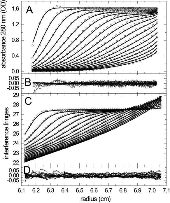
To test if the finite element model is suitable to describe experimental data, we globally fitted the sedimentation profiles obtained from a natural killer cell receptor Ly49C (31 kDa) interacting with MHC molecules H-2Kb (45 kDa) sedimenting at 50,000 rpm. As reported earlier, both the crystal structure and the solution interaction isotherm from the weight-average sedimentation coefficient distributions showed a 2:1 stoichiometry (44). Consistent with this, the shapes of the sedimentation profiles could be fitted very well globally over a large range of loading concentrations with a two-site binding model with equivalent and noninteracting sites and rapid reaction kinetics (Fig. 1). The best fit was found with a macroscopic K_D for site 1 of 1.7 μM, k_off = 0.1 s⁻¹, s_AB = 4.96 S, and s_ABB = 6.11 S, with a root-mean-square deviation (RMSD) of 0.0117 fringes. Convergence of the fit with the algorithm described above was practical with both Simplex and Levenberg-Marquardt methods, taking a few seconds on a 3-GHz PC per global simulation for the 10 data sets in the absence of back-diffusion.

FIGURE 1.

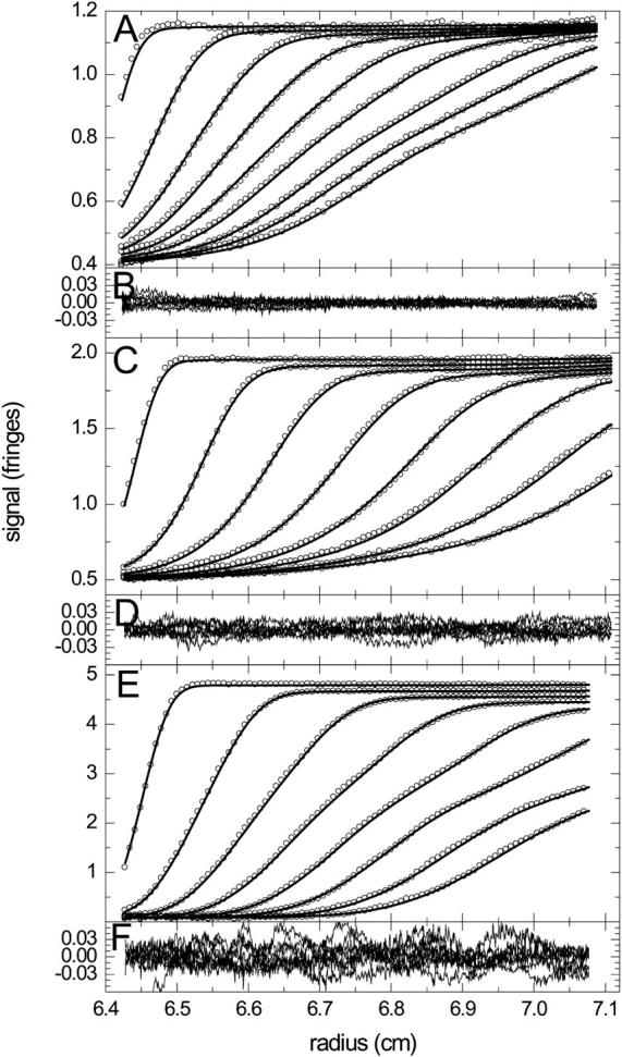
Experimental sedimentation profiles of the NK receptor Ly49C interacting with MHC class I molecules H-2Kb with a 1:2 stoichiometry (44). The data are from the global analysis of 10 separate experiments with a constant Ly49C concentration (4.97 μM) and variable MHC concentrations ranging from 1.2 to 28.7 μM. For clarity, only the experiments at 1.2 μM (A,B), 6.0 μM (C,D), and 28.7 μM (E,F) are shown (circles), and of those every 10th data point of every 7th (A,B) or 6th (B,C and E,F) scan, corresponding to time intervals of 1020 and 1130 s, respectively. For experimental details, see Dam et al. (44). The data were fitted with a two-step association model for noncooperative equivalent sites superimposed to a model for the redistribution of buffer salts and systematic baseline offsets. Best-fit distributions are shown as solid lines, with the macroscopic K_D for site 1 of 1.7 μM, and the off-rate constant of k_off = 0.1 s⁻¹. Overall rms deviation was 0.012 fringes, with the distribution of residuals indicated in panels B, D, and E.

Next, we examined how much detailed information on the interaction is contained in the sedimentation velocity profiles. With an incorrect model for a single site interaction, a 2.0-fold higher RMSD was obtained, in conjunction with an unreasonably high value for the s-value of the 1:1 complex (s_AB = 5.87 S). The ability to identify the correct sedimentation model should be expected because the isotherm of weight-average s-values as a function of loading composition already contains this information. However, a subtle but potentially important difference is that in this analysis the precise loading concentrations are floating parameters to be determined in the fit from the boundary shape, only constraining that the receptor concentration is the same by design of the experiment. In contrast, the k_off value was not found very well determined by the data; a fit with k_off = 0.0023/s produced an RMSD of 0.0118 fringes, only slightly higher than the best fit. However, when k_off was constrained to 10⁻⁵/s, the best-fit RMSD increased significantly to 0.0183 fringes, suggesting that for the given interaction set the approximate order of magnitude of the reaction kinetics may be discerned, but not the detailed rate constant.

The source of this limitation resides in the correlation of the sedimentation parameters and is due the small differences in the Lamm equation solutions for different k_off values in this range. This can be demonstrated by comparing simulated Lamm equation solutions in the absence of noise and radial-dependent and time-dependent baseline offsets. Noise-free data were simulated with the best-fit parameters of Fig. 1 for the complete set of 10 experiments at different loading concentrations, assuming a k_off value of 0.1/s. When k_off was fixed to the incorrect value of 0.001/s, a global fit with experimentally insignificant adjustments of the meniscus position and an only 5% change in K_D was found with a global RMSD of only 0.0044, which is smaller than the usual experimental noise.

A second experimental example is shown in Fig. 2, the sedimentation profiles of two peptides derived from the proline-rich domain of the adaptor protein SLP-76 and the SH3 domain of the enzyme phospholipase Cγ1 (PLC-γ), which play an essential role in signal transduction after T-cell activation (45). In contrast to the previous example, the two peptides have significantly different extinction coefficients (the only aromatic amino acid of the SLP-76 peptide is a single tyrosine), such that the dual signal data acquisition of absorbance at 280 nm and refractive index can report on each protein's sedimentation behavior in the mixture. This was exploited previously in a multiwavelength c(s) analysis, which showed the formation of a 1:1 complex (19). The evolution of the absorbance and interference signal profiles for a mixture is shown in Fig. 2, A and C, fitted with a kinetic Lamm equation model for 1:1 complex formation. It is apparent that the refractive index (RI) signal is superimposed by signal gradients from a low molecular weight component, likely buffer salts that sediment well below the range of s-values of interest, and are included in the model as an extra discrete species. Interestingly, in this multiwavelength analysis of a single experiment with each protein's buoyant molar mass, extinction coefficients and sedimentation coefficients determined separately, the binding constants appear already well determined. In a series of fits constraining the k_off value, K_D was found consistently ∼10 μM. The reaction kinetics was not very well determined, with RMSD of 0.0155 signal units (O.D. or fringes) for an instantaneous reaction, 0.0150 for k_off = 10⁻⁴/s, and 0.0137 for k_off < 10⁻⁵/s, and the best-fit value of 0.0136 for k_off = 1.6 × 10⁻⁶/s, although a slow reaction would be consistent with an expected large conformational change required for binding (46).

FIGURE 2.

Analysis of the interaction of peptides derived from the adaptor protein SLP-76 (11.7 kDa, 0.60 S) and PLC-γ (7.4 kDa, 0.75 S) which form complexes with 1:1 stoichiometry. SLP-76 contains only one tyrosine and no tryptophan residues, allowing its spectral discrimination from PLC-γ. Panels A and C show absorbance and interference profiles of a mixture (65 μM PLC-γ with 25 μM SLP-76) time intervals of 2500 s, at a rotor speed of 59,000 rpm and a temperature of 4°C (for clarity, only every 10th (A) or 20th (C) data point is shown). The interference optical data are superimposed by the sedimentation of a small buffer component (likely predominantly optically unmatched NaCl) which can be modeled well as discrete species at 0.055 S, as well as systematic baseline offsets accounted for by algebraic noise decomposition (41). Molar mass values were kept fixed at the values predicted from amino acid sequence, and extinction and sedimentation coefficients of free peptides were determined in prior experiments, but loading concentrations were fitting parameters. The residuals in panels B and D are from the fit with s_AB = 1.05 S, K_D = 10 μM and k_off = 10⁻⁵/s, with an RMSD of 0.0137.

After verifying that the sedimentation profiles of interacting systems predicted by the algorithm above is consistent with theory and experiment, we examine next the characteristic shapes displayed by the sedimentation boundaries of rapidly reversible systems.

Constant bath approximation as two noninteracting species

A well-known feature frequently found in the sedimentation of interacting two-component systems with dissimilar size and rapid kinetics is a characteristic bimodal boundary (see Figs. 1, 3, and 4), consistent with the predictions by Gilbert and Jenkins for the diffusion-free sedimentation of instantaneously reacting proteins (26). In the following we consider first mixtures with excess of the smaller component (A, 100 kDa) over a larger component (B, 200 kDa) or equimolar A and B. In this case, some of the free population of A sediments slower and forms the slow boundary, but a fraction of free A cosediments in the fast boundary. The free population of B, the complex population (AB), and a fraction of free A essentially cosediment in the fast boundary. This pattern was found independent of concentrations, except for c_A < c_B with c_B ≫ K_D. It is illustrated in Fig. 3 for equimolar A and B at different loading concentrations. In particular at low concentrations (Fig. 3 A) it is noticeable that the fast-sedimenting fraction of free A is very small, such that the fast boundary constantly migrates through regions where the concentration gradient of free A is relatively small. A quantitative example is highlighted in Fig. 3 B for equimolar loading concentrations at K_D; at the time point indicated by the bold lines, the boundary of free B increases from 10 to 90% of the plateau level within the dashed vertical lines. In the same region, the free A concentration changes only from 76 to 97% of its plateau level. Although this is a substantial increase, on the other hand, it should also be noted that the fast boundary is surrounded by at least 3/4 of the maximal free A throughout. Due to the mass action law, the gradient of free A causes changes in the fractional occupation of B amounting only to a range from 30 to 35%.

FIGURE 3.

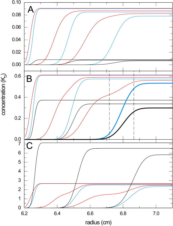
Theoretical distributions of free and complex species during the sedimentation of an interacting system A + B ↔ AB in the limit of instantaneous reaction. Total concentrations of components A and B were equimolar at 0.1-fold K_D (A), K_D (B), and 10-fold K_D (C). The profiles were calculated for a component A with 100 kDa and 7 S (red), component B with 200 kDa and 10 S (blue), forming a complex with 13 S (black). Sedimentation was simulated at a rotor speed of 50,000 rpm, and the profiles from time points 300, 1500, and 3000 s are superimposed. The vertical dashed lines in panel B indicate the radial range that covers 10–90% of the boundary of free B, and at the same time 76–97% of free A at 3000 s (indicated by bold lines).

FIGURE 4.

Total absorbance profiles for the simulated sedimentation of the system A + B ↔ AB in the limit of instantaneous reaction, as indicated in panel B of Fig. 3, at equimolar concentrations c_A = c_B = K_D (black solid lines), assuming extinction coefficients of 100,000 for components A and B. Shown are the theoretically predicted distributions without noise. The profiles are fitted to a model with two noninteracting species, as suggested by Eq. 5 for an ideal sedimentation/reaction process in a constant bath of A (red dashed lines). The best fit was found with parameters M*₁ = 88 kDa, s*₁ = 7.02 S for the slow boundary, and M*₂ = 198 kDa, and s*₂ = 11.15 S for the fast boundary, respectively, with an rms deviation of 0.0043 O.D.

This suggests that it is not unreasonable even for the interaction of two large proteins to examine how the sedimentation process relates to the ideal limiting case of sedimentation through a constant bath of the smaller component. The theoretical prediction is that, besides the boundary of the small component, the sedimentation exhibits a reaction boundary with a single sedimentation and diffusion coefficient that is characteristic for the reacting system. In Fig. 4, this prediction is tested by attempting a fit to the model of two noninteracting species, one corresponding to free A and one for the reacting system. As is visible in the small residuals in Fig. 4, this model can give an excellent description of the data. Similar fit qualities were found at other combinations of loading concentrations (data not shown). As predicted, the slower boundary sediments with a sedimentation coefficient very close to that of free A (7.02 S compared with 7.00 S underlying this simulation), and with a diffusion coefficient slightly higher than that of free A (∼12% higher, corresponding to an apparent molar mass of 88 kDa instead of 100 kDa). Similarly, the faster boundary migrates with an s-value of 11.15 S, which is very close to the weight-average s-value of 11.14 S predicted theoretically for this mixture (inserting the equilibrated loading concentrations into Eq. 6), but exhibits a 17% higher diffusion coefficient.

We examined the agreement of the sedimentation coefficients obtained from noninteracting species fits with those predicted by the constant bath theory over a range of concentrations (Fig. 5). The small s-value remains nearly constant at the value of free A, and the high s-value coincides very well with the isotherm predicted by Eq. 6. Further, we observed that the isotherm for the weight-average s-value of the reaction boundary predicted from Gilbert-Jenkins theory (35) is virtually superimposing that of Eq. 6. Therefore, we conclude that the constant bath approximation does indeed describe the essential features of the sedimentation process, and that the deviations mainly translate into excess boundary spreading. Although Fig. 5 is a direct comparison (without fitting) of the theoretically predicted isotherm Eq. 6 and the values obtained from a noninteracting species fit, it is obvious that modeling the latter with Eq. 6 should provide an excellent estimate of the association constant, for example, when using a dilution series with equimolar mixtures.

FIGURE 5.

Isotherm of the best-fit sedimentation coefficients for the slow and fast boundary components. The sedimentation process was simulated for the system A + B ↔ AB in the limit of instantaneous reaction (as described in Fig. 3), using equimolar concentrations of the components A and B. The calculated concentration profiles were fitted with a model for two noninteracting species, as shown in Fig. 4. The resulting sedimentation coefficients of the slow (□) and fast (•) boundary are plotted versus loading concentration (in units of K_D). For comparison, the solid line shows the isotherm Eq. 6 theoretically expected in the ideal limit of sedimentation a constant bath of the slow component. The dashed blue line shows the isotherm calculated by Gilbert-Jenkins theory as described in Dam and Schuck (35).

A concentration regime where these considerations do not hold true is that of molar excess of the larger component at concentrations far above K_D. In this limit, the two characteristic sedimentation and diffusion coefficients will reflect those of B and the complex AB, and the concentration gradients of A comigrating with the boundary AB will be large. For example, with A at threefold and B fivefold K_D, respectively, the change of relative concentration of A in the fast boundary are >50%. In summary, as is illustrated in Figs. 3–5, the constant bath approximation is applicable for the equimolar case, and for molar excess of A over B, but not for molar excess of B over A.

Sedimentation coefficient distributions c(s) of reactive systems

Next, we examined the application of the sedimentation coefficient distribution c(s) to the sedimentation of reacting systems (Fig. 6). From the considerations above it is not surprising that for fast reactions, it shows two peaks, and that the quality of fit is very good. In contrast to the conventional interpretation of c(s) peaks to reflect the sedimentation of different species, for fast-reacting systems they reflect the characteristic sedimentation coefficients of the sedimenting system. For example, for equimolar mixtures in Fig. 6 A, the peak at the smaller s-value remains constant at the sedimentation coefficient of the smaller component, whereas the second peak shows a concentration dependence. The integration of the faster peak gives the s-value of the reaction boundary, and nonlinear regression with the isotherm predicted by Eq. 6 leads to the correct K_D value with a precision better than 2%. Similar results are obtained for a titration series of a constant amount of B with varying A (Fig. 6 B), and even for a titration series of constant A with varying B (Fig. 6 C). Although we found the constant bath approximation to poorly describe the sedimentation for c_B ≫ K_D at molar excess of B, which produces bimodal c(s) (dotted and dashed-dotted lines in Fig. 6 C), the isotherm analysis is surprisingly robust and still gives reasonable estimates of K_D if the s-value of the complex is constrained.

FIGURE 6.

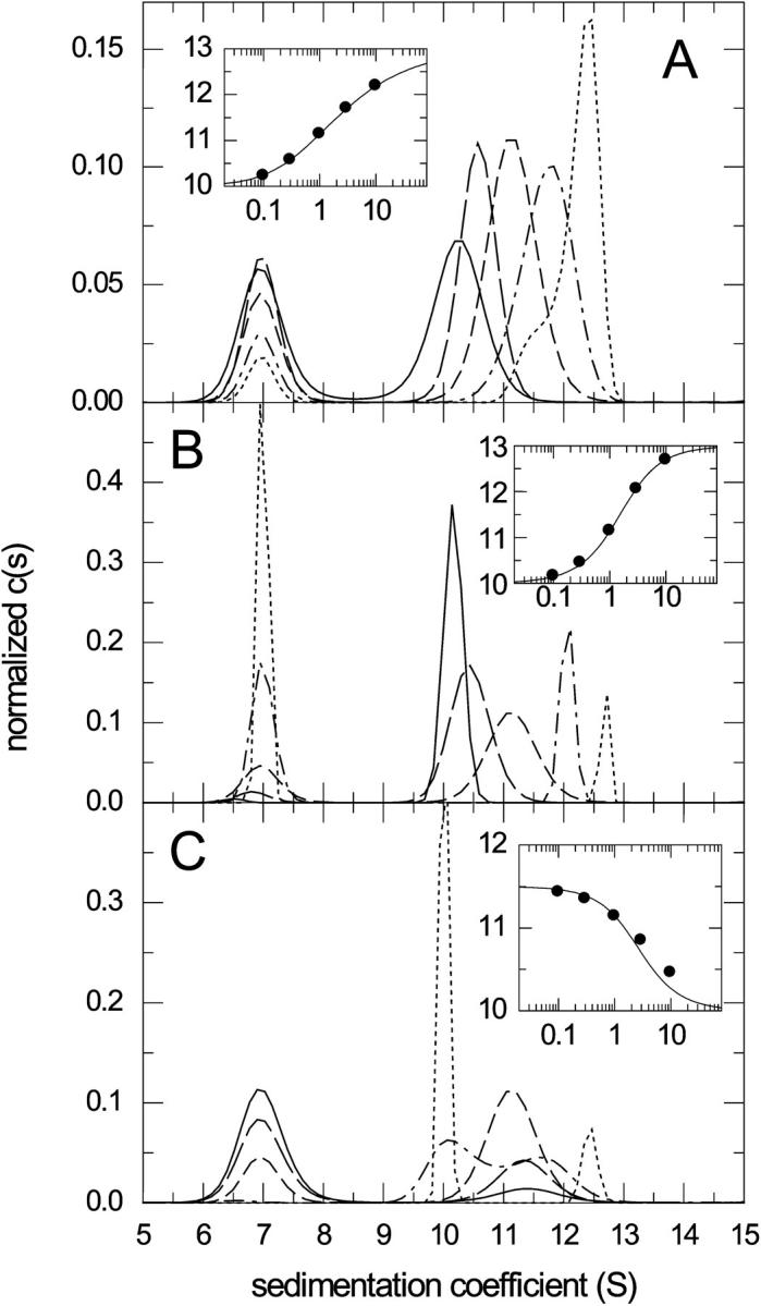
Sedimentation coefficient distributions c(s) of noninteracting species calculated from the sedimentation profiles of the reacting system A + B ↔ AB in the limit of instantaneous reaction (Fig. 3). The c(s) distributions are normalized to unit area, and calculated for concentration series of 0.1-fold (solid line), 0.3-fold (long dashed line), onefold (short dashed line), threefold (dashed-dotted line), and 10-fold (dotted line) K_D, respectively. Panel A shows the distributions for equimolar concentrations, panel B with a constant larger component at K_D titrated by the smaller component, and panel C vice versa with a constant smaller component at K_D titrated by the larger component. The insets show the best-fit isotherms of Eq. 6 (lines) to the weight-average s-value of the fast boundary component determined by integrating the c(s) distribution between 9 and 13 S (symbols), resulting in binding constants within 3% of the correct K_D underlying the simulation.

We compared the error estimates of the analysis with the isotherm Eq. 6 and the conventional analysis of the weight-average s-value. In the titration of constant B with varying A (Fig. 6 B), if the s-value of the complex s_AB is treated as an unknown in the analysis of the isotherm, the error estimates for s_AB were found fourfold smaller as compared to the conventional isotherm analysis of the overall weight-average s-value (data not shown), and error estimates for K_D were threefold better. A global analysis led only slight further improvement.

The boundary shapes are interpreted in the c(s) method as if originating from noninteracting species, with a relationship D(s) scaled via a single average frictional ratio. As described above, the sedimentation boundary in most configurations does fit the predicted two noninteracting species sedimentation very well. As a consequence, the deconvolution of diffusion in the c(s) should work properly if applied to these reaction boundaries. The deviations from the “constant bath” sedimentation causes that the boundary components have larger apparent diffusion coefficients. In the c(s) method, we found that this can translate into smaller f/f_o values than would be expected from the known hydrodynamic shapes of the components. Therefore, besides the obvious concentration dependence of c(s) at different loading concentrations, too low f/f_o values can therefore be taken as an indication of the presence of a reaction on the timescale of sedimentation. A second, more subtle effect of deviations from the “constant bath reaction” is that the peaks appear slightly broader and/or asymmetric. For example, the fast peak indicated by the dotted line in Fig. 6 A would suggest a bimodal peak and the presence of a second, slightly smaller component. Similarly, we found that intermediate peaks in trace concentrations can occur. For reaction boundaries, therefore, whereas the c(s) method correctly describes the characteristic s-values of the system and can be combined with a quantitative analysis of the isotherms of the fast component s-value, the shape of c(s) cannot be interpreted to the same level of detail as is possible with noninteracting mixtures.

Next, we studied slower reactions. The parameter governing the sedimentation pattern is the chemical off-rate constant k_off. For k_off > 0.01/s, at rotor speeds that can be experimentally achieved, we observed sedimentation boundaries nearly identical to those of instantaneous reactions. For slow reactions with k_off < 10⁻⁵ s, the limit of stable reactions on the timescale of sedimentation was approached (rms deviation < 0.1%). In between, the sedimentation profiles gradually transform from a bimodal boundary with the characteristic s-values described above for fast reactions, to a trimodal boundary reflecting the s-values of the populated species for slow reactions. Insofar as the boundary shape is reflected in the apparent sedimentation coefficient distributions ls-g*(s), the transition is shown in the dotted lines in Fig. 7 (for equimolar concentration equal to K_D). At high reaction rates, the fast boundary component exhibits the single peak expected for fast reactions (black dotted line is based on instantaneous reaction), which splits up into two fast peaks (10 and 13 S) for slow reactions (magenta dotted line for k_off = 10⁻⁵/s). The results of the sedimentation coefficient distribution c(s) are shown in Fig. 7 as solid lines. The peaks are sharper because of the deconvolution of diffusion. With decreasing reaction rate constant they also display the transition where the reaction boundary (black bold line) splits up into two sharp peaks (magenta bold line) reflecting the separate populations of B and AB. The intermediate kinetics with rate constants of 10⁻³–10⁻⁴/s is of particular interest because it is far from the special cases mimicking noninteracting species. In this regime, the boundary shapes deviate most from those of noninteracting species (due to the similarity of the fast reaction boundary with a discrete species; see above), and, as a consequence, the deconvolution of the boundary shapes in terms of diffusion as implemented in the c(s) approach appears most problematic. We found for k_off ∼ 10⁻³/s the c(s) distributions are close to those of the fast reactions, at k_off ∼ 3–6 × 10⁻⁴/s a bimodal pattern sets in (long dashed green and cyan lines), and at k_off ∼ 10⁻⁴/s the species peaks are already baseline separated, although the correct s-values are not yet established. This shows that despite the influence of the reaction kinetics on the boundary shape, the diffusional deconvolution is still partially effective.

FIGURE 7.

Sedimentation coefficient distributions from the simulated sedimentation of the interacting system A + B ↔ AB with different reaction rate constants, at equimolar concentrations equal to K_D. Shown are c(s) distributions of diffusing species with maximum entropy regularization (solid and dashed lines, left ordinate) and for comparison, the apparent sedimentation coefficient distributions ls-g*(s) (dotted lines). Reaction rate constants are: log₁₀(k_off) = −5 (magenta), −4 (light green), −3 (red), −3.5 (dashed cyan), −3.2 (dashed green), −2 (blue), and instantaneous (black). Sedimentation parameters are as those in Fig. 3.

This transition and the resulting c(s) distributions were studied in more detail. Fig. 8 shows the sedimentation coefficient distributions for k_off = 1 × 10⁻³/s, 4 × 10⁻⁴/s, and 1 × 10⁻⁴/s the effect of different loading concentrations (equimolar). At k_off = 10⁻³/s (panel A) the boundaries are still similar to the fast reaction limit shown in Fig. 6 A in that they show a single reaction boundary at low concentration, which tends to split up only at higher concentrations. The isotherm of the weight-average s-value of the fast boundary component can still be modeled well with the “constant bath” approximation (inset in Fig. 8 A), leading to an underestimate of K_D by 21%. At k_off = 4 × 10⁻⁴/s, the reaction is already slow enough for species populations to be discerned by c(s). Correspondingly, the reaction boundary cannot be modeled very well with a single s- and D-value (data not shown). Integration of both peaks with s > 8.5 S and data analysis with Eq. 6 results in an underestimate of K_D by 32%. The relative peak areas of the free A, free B, and complex peaks can be modeled well with the isotherm of partial concentrations determined by mass action law and mass balance, which describes the species populations in the limit of an initially equilibrated mixture that does not react during the sedimentation. This resulted in an underestimate of K_D by 15%. Finally, at k_off = 10⁻⁴/s the species boundaries appear already fully separated in c(s); c(s) peaks for each species appear approximately at constant position. Again, this separation is not observed for the ls − g*(s) distribution, which means the resolution of species can be attributed entirely to the diffusional deconvolution. The partial populations from integration of c(s) peaks also can be well described with the species population isotherms, leading to an overestimate of K_D by 13%. These results confirm that the diffusional deconvolution applied in the c(s) analysis is partially effective even for reaction-controlled boundaries. They appear to be quantitatively reasonably precise in the average s-value of the fast boundary component when no peaks can be discerned, and even in the partial species concentrations when peaks can be distinguished. However, the exact peak positions should not be interpreted as they do not reflect either the true s-values of the sedimenting species, or a characteristic s-value of the reacting system.

FIGURE 8.

Sedimentation coefficient distributions c(s) at different concentrations for the transition from a single fast reaction boundary component to a split, species dominated boundary shape. Sedimentation conditions are as described in Fig. 3, and concentrations are as indicated in Fig. 6 ranging from 0.1-fold (solid line) to 10-fold K_D (dotted line). Reaction rate constants are log₁₀(k_off) = −3 (A), −3.4 (B), and −4 (C). The insets are analysis of the isotherms of the reaction boundary with a constant bath model (A and B; symbols are values from integration of c(s) from 8.5 to 14 S, solid line is best-fit isotherm with Eq. 6), and the isotherms of the partial populations of the individual species (determined by integration of c(s) from 5.5 to 8.5 (▪), 8.5–11.6 (▵), and 11.6–14 S (○), respectively) (B and C). Modeling the isotherms led to estimates for the equilibrium dissociation constants of 0.79 K_D (A), 0.85 K_D (B; population isotherm), and 1.13 K_D (C).

The deconvolution of diffusion from reaction boundaries is further studied in the application to the interaction of small proteins. Fig. 9 shows the c(s) profiles for a fast reaction (k_off = 0.01/s; panel A) and a slow reaction (k_off = 3 × 10⁻⁵/s; panel B) of a 25-kDa, 2.5-S protein binding to a 40-kDa, 3.5-S protein forming a 5-S complex. As indicated by the ls-g*(s) curves shown with offset, for both situations the shape of the sedimentation boundary is governed by diffusion and does not allow species or reaction boundaries to be discerned. For the fast reaction, the c(s) analysis results in curves showing an undisturbed peak at 2.5 S and a concentration-dependent reaction boundary, which can be modeled well with the isotherm Eq. 6 (with a best-fit K_D 1.01-fold of that underlying the simulations). An exception is the curve at the lowest concentration, for which the signal/noise ratio is too low and the regularization causes a single peak (which was omitted in the isotherm analysis). This situation is very similar to that obtained for larger species (Fig. 6 A). For the slow reaction, again, at the lowest concentrations c(s) does not result in resolved peaks for each species, but at the higher concentrations the species peaks with concentration-dependent heights are obtained, analogous to Fig. 8 C. For both the slow and fast reaction, in addition to the requirement of higher signal/noise ratio, resolving the boundaries was found only possible if sedimentation data were included from long observation times spanning the complete migration of the slowest boundary through the experimentally accessible radial observation range.

FIGURE 9.

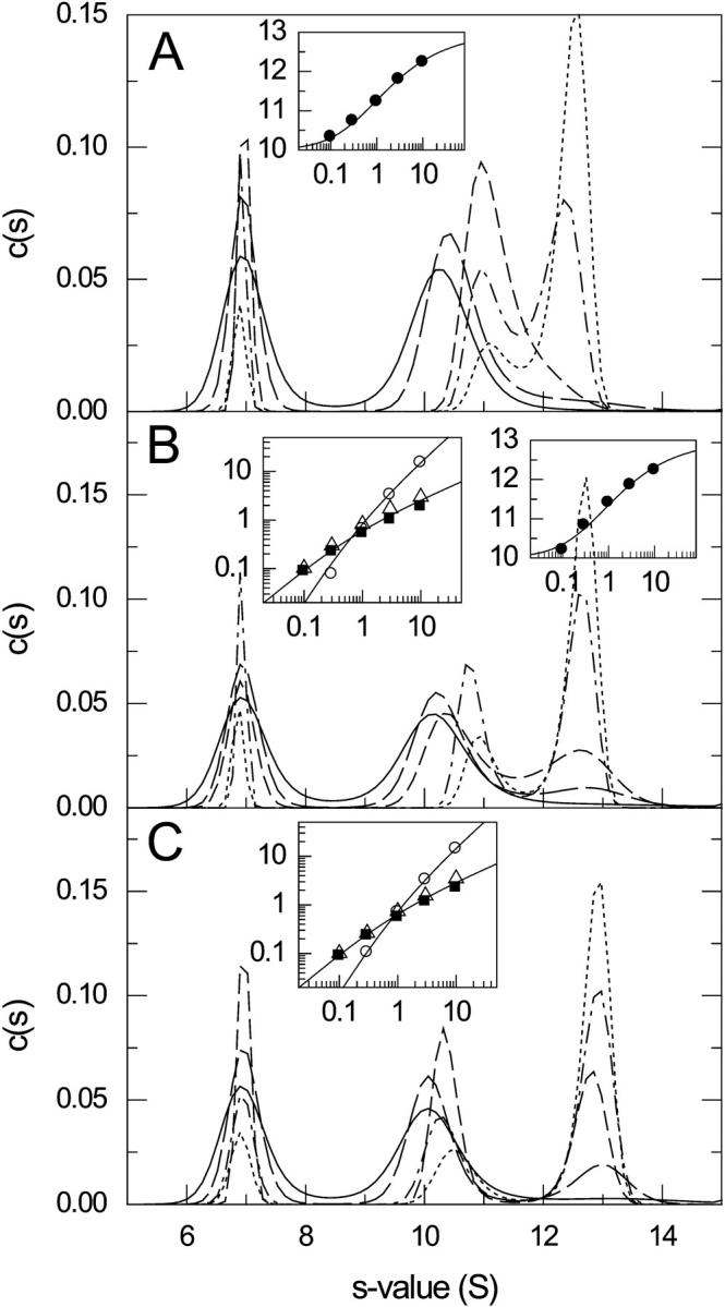
Shown are c(s) distributions from a system of two reversibly associating small proteins. Sedimentation was simulated for a protein of 25 kDa, 2.5 S binding to a 40 kDa, 3.5-S species forming a 5-S complex with K_D = 3 μM. Data were simulated for an interference optical experiment at 50,000 rpm with typical signal/noise ratio, with 60 scans over a time interval of 5 h. Concentrations were 0.3 (solid line), 1 (long dashed line), 3 (short dashed line), 10 (dashed-dotted line), and 30 μM (dotted line) equimolar. Distributions were calculated with maximum entropy regularization with P = 0.7. (A) Fast reaction with k_off = 0.01/s. The inset shows as circles the weight-average s-value of the fast boundary component from integration of c(s) (except for the lowest concentration, where a second boundary component could not be discerned). The solid line in the inset is the best-fit constant bath isotherm Eq. 6, resulting in a K_D estimate of 3.4 μM and complex s-value of 5.06 S. (B) Slow reaction with k_off = 3 × 10⁻⁵/s. For comparison, results from the ls − g*(s) are shown as thin lines, offset by 1.5 fringes/s. All distributions are normalized to have equal area.

DISCUSSION

Goal of this work was to develop new theoretical tools for the study of protein interactions by sedimentation velocity. We have first derived improved algorithms to compute Lamm equation solutions of interacting systems, which can be fitted to experimental sedimentation data. Subsequently, this was used to examine the “constant bath” approximation of sedimentation of a rapidly interacting system with a vanishing concentration gradient of one component. A result of this limiting case is that the reaction boundary exhibits a single diffusion coefficient. This provided the background for the study of c(s) distributions, in particular, to understand why the property of c(s) of deconvoluting diffusion remains successful in the presence of fast reactions. Finally, we have examined the result of c(s) analyses applied to sedimentation boundaries of systems with finite reaction rates, and characterized the transition of c(s) peaks from reporting reaction boundaries to species populations. For both cases, robust isotherm models were derived. The case of rapidly reacting systems will be further explored in the accompanying article (35), which compares c(s) with the asymptotic boundary profiles from Gilbert-Jenkins theory (26) and derives more detailed isotherms for height and s-values of both the undisturbed and the reaction boundary computed by c(s).

Solving the Lamm equation for reactive system has a long tradition, both for simulation of boundary shapes and for modeling of data (4–6,8,11,30,31,43,47–50). We have developed an algorithm with adaptive time-step control, and a predictor-corrector scheme in which the reaction and migration fluxes are coupled. Because the sharp concentration gradients close to the bottom of the cell can create numerical instabilities (exacerbating those observed for single component Lamm equation solutions (51)), we have derived finite element Lamm equation solutions for a semiinfinite cell. Usually, the back-diffusion is excluded from the fitted sedimentation data because of potential aggregation or phase transitions at the high local concentration at the surface of the centerpiece, which would affect the concentration distribution in the back-diffusion range. As a consequence, likewise, the effect of this solution boundary does not need to be included in the Lamm equation solution. Back-diffusion may not be excluded when studying small proteins where this is a significant feature of the sedimentation profiles. However, in this case the concentration gradients at the bottom of the cell are much smaller. For this reason, in the implementation in SEDPHAT back-diffusion can be optionally excluded (dependent on the experimental data), which can lead to significantly increased stability and efficiency of the Lamm equation solution for large proteins.

The calculated sedimentation profiles (assuming typical experimental conditions) show a dependence on the reaction rate constant in the range from k_off = 10⁻²/s to ∼10⁻⁵/s, with k_off = 10⁻²/s close to the ideal case of an instantaneous reaction, and k_off = 10⁻⁵/s close to a stable reaction. This is consistent with previous findings (52,53). The shape of the sedimentation profiles will depend on both the on-rate constant k_on and the dissociation rate constant k_off, as the reaction will be governed by the relaxation constant k_rel = k_off + k_on(c_a + c_b). This dependence is expressed in this work as a dependence on protein concentrations relative to the equilibrium constant K_D = k_off/k_on, i.e., the fractional equilibrium population of the different species, which permits the concentration-dependent sedimentation behavior in this work to be categorized according to the dissociation rate constant k_off. Nevertheless, it should be noted that reassociation can readily occur during the sedimentation velocity experiment, because the faster sedimenting complexes are maintained throughout in a bath of the slower sedimenting free components.

Although the Lamm equation solutions can be used to globally model experimental data and to estimate kinetic rate constants, as illustrated in Fig. 1, we found that the rate constant is not always very well determined by the data. For small proteins that exhibit high diffusional spread, the difference between sedimentation profiles calculated for fast or slow reactions in the global model can be on the order of the noise of the data acquisition. This can be more problematic if the reaction scheme is not conclusively established and alternate sedimentation models are considered (such as monomer-dimer-tetramer versus monomer-tetramer associations, data not shown). In this case, independent information from other methods on either the reaction scheme or the kinetic timescale may be required. In this regard, it might be considered that many or even most physiologically relevant protein interactions with affinities in the micromolar range have a fast kinetics (high k_off) on the timescale of sedimentation. However, there are also many examples of complexes with low k_off and relatively low k_on: Complex formation in vivo may be driven by local concentrations of reactants, dissociation may be dependent on cofactors, or the interactions may be accompanied by conformational changes and require activation energy. In practice, a useful qualitative indicator for the presence a slow reaction can be the ability to separate the complexes by size-exclusion chromatography.

Fig. 2 is an example of exploiting multisignal detection, taking advantage of differences in the extinction coefficients of the binding partners by simultaneous acquisition of interference optical refractive index data and absorbance data at 280 or 250 nm. For many proteins, this approach may not require extrinsic labeling (19). It was shown recently how multisignal detection can facilitate the determination of complex stoichiometries in the multisignal c_k(s) analysis (19). Multisignal detection provides an additional data dimension that can be highly advantageous to determine binding constants, and to discriminate between different reaction models of heterogeneous interactions.

Although it appears that the modeling of experimental data with Lamm equation solutions for reactive systems may be the most comprehensive and rigorous approach to study protein interactions by sedimentation velocity without theoretical approximations, the potentially small differences in the boundary shapes from different reaction rate constants suggest that it may also be most susceptible to experimental imperfections. An example of the susceptibility of the extraction of information from boundary shapes by Lamm equation modeling to imperfect data can be found in (42), where the sedimentation profiles from a preparation of protein potentially exhibiting microheterogeneity from glycosylation and including small percentages of both smaller (5%) and larger (8%) molecular weight impurities are used as an illustration: When the boundary shapes are modeled with a single species Lamm equation solution, a qualitatively wrong molar mass value is obtained (63 kDa), even though the residuals of the fit are below 0.01 fringes. In contrast, partially sacrificing the precise information on the diffusional boundary spread in the c(s) method (by extracting only a weight-average frictional ratio and assuming a hydrodynamic scaling law), a sedimentation coefficient distribution can be obtained that displays the heterogeneity of the sample, gives a better fit, and leads to a molar mass estimate of 93 kDa. Although the latter estimate is inherently less rigorous and less precise due the scaling law assumptions used in its derivation, this value still allows correctly to deduce the oligomeric state of the protein, whereas the estimate from single-species Lamm equation modeling could not. Although this example is taken from the analysis of a noninteracting protein, it illustrates the well-known susceptibility of the boundary shape to heterogeneity (even at trace levels), which, if unaccounted for, can lead to substantial errors in the parameters describing the boundary spread. Similarly, Cann has discussed previously the profound effects of microheterogeneity in the binding constants on the shape of the sedimentation boundaries (55). Further, Werner and Schachman have described the influence of conformational heterogeneity on the shape of the sedimentation boundary (56). As a consequence, if factors are not recognized, a Lamm equation model that interprets the boundary shape only in terms of diffusion and reaction kinetics may arrive at incorrect parameter estimates.

Further, modeling of experimental data with Lamm equation solutions for reactive systems is computationally complex and time-consuming, and requires a model for the interaction and good starting guesses for the parameters to be established. Therefore, it is important to study robust alternative approaches, which can extract qualitative kinetic information, allow quantitative thermodynamic analysis of binding constants, and characterize the hydrodynamic parameters of the sedimenting species.

Finite element solutions of the Lamm equation were used to examine the “constant bath” theory, which was originally devised for protein-small molecule interactions, and studied here with the goal to test its predictions for medium-sized proteins. Although the assumption of a negligible gradient of the smaller component seems difficult to achieve in theory, interactions at finite rate constants can be expected to exhibit smaller gradients than those of instantaneous reactions considered here (e.g., Fig. 3), and experimental systems where such gradients were absent have been described (54). The result of the “constant bath” approximation that the reaction boundary sediments with a single sedimentation and a single diffusion coefficient seems to contradict the well-known predictions by Gilbert-Jenkins theory on the asymptotic boundary shapes (26). However, it should be noted that both theories neglect different essential features of the sedimentation process to arrive at analytically tractable and insightful limiting cases. The “constant bath” theory neglects concentration gradients of one species, free A, which if considered would lead to some heterogeneity in the ratio of complex AB/B, and as a result lead to some dispersion in the s-value of the reaction boundary. On the other hand, the most important simplification of Gilbert-Jenkins theory is the absence of diffusion, which if considered would diminish the concentration gradients across the reaction boundary. Despite the differences in approach, the concentration dependence of the s-value of the reaction boundary shown in Fig. 5 is virtually identical. Furthermore , that the “constant bath” theory can be a realistic approximation for the reaction between dissimilar-sized proteins (with molar masses differing by twofold or more, and where component A is far from saturation), is supported by the agreement between the isotherms of the s-value of the fast boundary components with Eq. 6.

From the background of the “constant bath” approximation, it is not surprising that diffusion can be deconvoluted from the reaction boundaries of rapidly interacting systems using the c(s) method. It also follows that the c(s) traces have to be regarded in the context of a family of c(s) curves obtained at different loading concentrations. Only this can permit to differentiate between noninteracting and rapidly interacting species (as demonstrated by Fig. 4). That there remains a finite gradient of free A across the reaction boundary translates in diffusion coefficients slightly higher than predicted by the “constant bath” approximation, and slightly broader c(s) profiles than would be expected for noninteracting species. A comparison of these c(s) profiles with the asymptotic velocity gradients predicted by Gilbert-Jenkins theory will be made in the accompanying article. The performance of c(s) extracting peaks corresponding to reaction boundaries is highlighted in Fig. 9 A, which allows the diagnostics of the kinetic regime of the reaction, in contrast to the apparently feature-less diffusion broadened sedimentation profiles of small species and their corresponding g*(s) curves. It should be noted that for small species, at low concentrations the resolution of c(s) can be limited by a low signal/noise ratio of the data, and the regularization merging neighboring peaks.

The “constant bath” theory opens the possibility for using the isotherm of the s-value of the reaction boundary Eq. 6 as an analytical tool. In comparison to the weight-average s-value, the reaction boundary is closer to the s-value of the complex, and therefore permits a better estimate of the s-value of the complex, which is frequently a difficult task. This confirms the utility of using the concentration dependence of the fast reaction boundary as a quantitative analysis tool, as reported earlier (32), and demonstrates that it can be applied also in combination with the high resolution of the diffusion-deconvoluted sedimentation coefficient distributions of c(s).

However, it cannot be applied to titrations including excess of the larger component over the smaller. A global analysis of the weight-average and the reaction-boundary s-value has been implemented in SEDPHAT. (In this context, it is also interesting to note that the s-value of the reaction boundary according to Eq. 6 is not dependent on extinction coefficients or signal increments, whereas the weight (or signal-average, respectively) is. This topic will be further explored in comparison with the asymptotic Gilbert-Jenkins boundaries, from which a more general model for the s-value of the reaction boundary and additional isotherms for the height of the undisturbed and the reaction boundary will be derived (35).

In the limit of slow reactions, the c(s) distribution results in peaks at positions largely independent of concentration, but with relative areas reflecting the populations of the individual sedimenting species. This is equivalent to the absence of chemical reaction during the sedimentation velocity experiment (except for initial equilibration of species), and diffusion is deconvoluted as in the conventional case of noninteracting mixtures (Fig. 9 B). We have implemented in SEDPHAT isotherm analysis models for species populations, to conveniently use this information to determine binding constants. This could be advantageous in comparison with the analysis of weight-average s-values.

For practical experimental conditions, the transition from sedimentation governed by the reacting system to sedimentation of individual species was found to occur over a relatively narrow range of kinetic rate constants, with k_off ∼ 0.0001–0.001/s (Fig. 8). No simplifying theoretical limiting case exists for sedimentation in this kinetic regime. Using c(s) for deconvolution of diffusion, we observed the transition from fast to slow reactions as a reaction boundary that acquires at lower rate constant a bimodal shape (first at the higher concentrations), which at still lower rate constants form the species peaks at concentration-independent positions. It should be noted that at k_off ∼ 0.0001/s, even though the c(s) peaks corresponding to the complex the s-values of the peak can be clearly discerned at a virtually concentration-independent position, they are not sufficiently precise to permit hydrodynamic modeling of the complex shape. This would require either lower rate constants or higher fractional saturation of the complex. Interestingly, however, modeling the boundaries in this transition regime with the isotherms derived for the reaction boundary of rapidly reacting systems, or, where species peaks can be discerned, with the isotherm for the populations of stable species, does not lead to large errors. The robustness of these models supports that the underlying concepts for interpreting the boundary shapes, the deconvolution of diffusion, and the interpretation of the resulting peaks in c(s) still can be applied in this kinetic regime.

We have examined two methods to analyze sedimentation velocity experiments from interacting systems, the direct modeling of Lamm equation solutions of reactive systems, and the c(s) approach to determine the underlying sedimentation coefficient distributions. For physical reasons of the ultracentrifugation experiment, both are most sensitive to reaction kinetics in the range of k_off ∼ 0.0001–0.001/s. The Lamm equation modeling does not require theoretical approximations but makes assumptions about the reaction scheme, and requires the absence of unaccounted species contributing to the broadening of the sedimentation boundary. Using detailed information on species diffusion coefficients, the boundary shapes are modeled to obtain parameter estimates for the kinetic rate constants. In contrast, the c(s) approach uses the boundary shape information only to approximately deconvolute the effect of diffusion from the reaction boundaries, and to extract the underlying sedimentation coefficient distributions. Only order-of-magnitude estimates of the kinetic rate constants are possible insofar as they significantly influence the sedimentation coefficient distribution, but no assumption is necessary regarding the number of species in solution (and regarding the absence of microheterogeneity), and the presence of species outside the range of the interacting proteins will be revealed as part of the result. The methods are complementary, and whether a given set of experiments can be interpreted with explicit Lamm equation solutions of a reactive system, or some details of boundary shape information should be sacrificed to account for sample heterogeneity will depend on the particular system under investigation. It should be noted that these methods are not exclusive, and a c(s) approach, because it is easier to apply, can be utilized also as a preliminary step for the Lamm equation modeling, to demonstrate the suitability of the material for the more rigorous analysis, develop a model for the interaction scheme, and to derive starting estimates of the parameters.

References

- 1.Svedberg, T., and K. O. Pedersen. 1940. The Ultracentrifuge. Oxford University Press, London, UK.
- 2.Lamm, O. 1929. Die Differentialgleichung der Ultrazentrifugierung. Ark. Mat. Astr. Fys. 21B:1–4. [in German]. [Google Scholar]
- 3.Holladay, L. A. 1979. An approximate solution to the Lamm equation. Biophys. Chem. 10:187–190. [DOI] [PubMed] [Google Scholar]
- 4.Gilbert, G. A., and L. M. Gilbert. 1980. Ultracentrifuge studies of interactions and equilibria: impact of interactive computer modelling. Biochem. Soc. Trans. 8:520–522. [DOI] [PubMed] [Google Scholar]
- 5.Urbanke, C., B. Ziegler, and K. Stieglitz. 1980. Complete evaluation of sedimentation velocity experiments in the analytical ultracentrifuge. Fresenius Z. Anal. Chem. 301:139–140. [Google Scholar]
- 6.Cox, D. J., and R. S. Dale. 1981. Simulation of transport experiments for interacting systems. In Protein-Protein Interactions. C. Frieden and L. W. Nichol, editors. Wiley, New York, NY.
- 7.Philo, J. S. 1997. An improved function for fitting sedimentation velocity data for low molecular weight solutes. Biophys. J. 72:435–444. [DOI] [PMC free article] [PubMed] [Google Scholar]
- 8.Kindler, B. 1997. Akkuprog: Auswertung von Messungen chemischer Reaktionsgeschwindigkeit und Analyse von Biopolymeren in der Ultrazentrifuge. University of Hannover, Hannover, Germany. [in German].
- 9.Schuck, P. 1998. Sedimentation analysis of noninteracting and self-associating solutes using numerical solutions to the Lamm equation. Biophys. J. 75:1503–1512. [DOI] [PMC free article] [PubMed] [Google Scholar]
- 10.Demeler, B., J. Behlke, and O. Ristau. 2000. Determination of molecular parameters from sedimentation velocity experiments: whole boundary fitting using approximate and numerical solutions of the Lamm equation. Methods Enzymol. 321:36–66. [DOI] [PubMed] [Google Scholar]
- 11.Stafford, W. F., and P. J. Sherwood. 2004. Analysis of heterologous interacting systems by 36 sedimentation velocity: curve fitting algorithms for estimation of sedimentation coefficients, equilibrium and kinetic constants. Biophys. Chem. 108:231–243. [DOI] [PubMed] [Google Scholar]
- 12.Cole, J. L., and J. C. Hansen. 1999. Analytical ultracentrifugation as a contemporary biomolecular research tool. J. Biomol. Tech. 10:163–176. [PMC free article] [PubMed] [Google Scholar]
- 13.Arisaka, F. 1999. Applications and future perspectives of analytical ultracentrifugation. Tanpakushitsu Kakusan Koso. 44:82–91. [PubMed] [Google Scholar]
- 14.Laue, T. M., and W. F. I. Stafford. 1999. Modern applications of analytical ultracentrifugation. Annu. Rev. Biophys. Biomol. Struct. 28:75–100. [DOI] [PubMed] [Google Scholar]
- 15.Rivas, G., W. Stafford, and A. P. Minton. 1999. Characterization of heterologous protein-protein interactions via analytical ultracentrifugation. Methods. 19:194–212. [DOI] [PubMed] [Google Scholar]
- 16.Lebowitz, J., M. S. Lewis, and P. Schuck. 2002. Modern analytical ultracentrifugation in protein science: a tutorial review. Protein Sci. 11:2067–2079. [DOI] [PMC free article] [PubMed] [Google Scholar]
- 17.Scott, D. J., and P. Schuck. 2005. A brief introduction to the analytical ultracentrifugation of proteins for beginners. In Modern Analytical Ultracentrifugation: Techniques and Methods. D. J. Scott, S. E. Harding, and A. J. Rowe, editors. The Royal Society of Chemistry, Cambridge, UK. In press.
- 18.Balbo, A., and P. Schuck. 2005. Analytical ultracentrifugation in the study of protein self-association and heterogeneous protein-protein interactions. In Protein-Protein Interactions. E. Golemis and P. D. Adams, editors. Cold Spring Harbor Laboratory Press, Cold Spring Harbor, New York, NY. In press.
- 19.Balbo, A., K. H. Minor, C. A. Velikovsky, R. Mariuzza, C. B. Peterson, and P. Schuck. 2005. Studying multi-protein complexes by multi-signal sedimentation velocity analytical ultracentrifugation. Proc. Natl. Acad. Sci. USA. 102:81–86. [DOI] [PMC free article] [PubMed] [Google Scholar]
- 20.van Holde, K. E., and W. O. Weischet. 1978. Boundary analysis of sedimentation velocity experiments with monodisperse and paucidisperse solutes. Biopolymers. 17:1387–1403. [Google Scholar]
- 21.Demeler, B., H. Saber, and J. C. Hansen. 1997. Identification and interpretation of complexity in sedimentation velocity boundaries. Biophys. J. 72:397–407. [DOI] [PMC free article] [PubMed] [Google Scholar]
- 22.Stafford, W. F. 1992. Boundary analysis in sedimentation transport experiments: a procedure for obtaining sedimentation coefficient distributions using the time derivative of the concentration profile. Anal. Biochem. 203:295–301. [DOI] [PubMed] [Google Scholar]
- 23.Schuck, P., and P. Rossmanith. 2000. Determination of the sedimentation coefficient distribution by least-squares boundary modeling. Biopolymers. 54:328–341. [DOI] [PubMed] [Google Scholar]
- 24.Schuck, P. 2000. Size distribution analysis of macromolecules by sedimentation velocity ultracentrifugation and Lamm equation modeling. Biophys. J. 78:1606–1619. [DOI] [PMC free article] [PubMed] [Google Scholar]
- 25.Gilbert, G. A. 1955. Faraday Discuss. 20:68–71. [Google Scholar]
- 26.Gilbert, G. A., and R. C. Jenkins. 1956. Boundary problems in the sedimentation and electrophoresis of complex systems in rapid reversible equilibrium. Nature. 177:853–854. [DOI] [PubMed] [Google Scholar]
- 27.Steiner, R. F. 1954. Reversible association processes of globular proteins. V. The study of associating systems by the methods of macromolecular physics. Arch. Biochem. Biophys. 49:400–416. [DOI] [PubMed] [Google Scholar]
- 28.Fujita, H. 1975. Foundations of Ultracentrifugal Analysis. John Wiley & Sons, New York, NY.
- 29.Goad, W. B., and J. R. Cann. 1969. Theory of sedimentation of interacting systems. Ann. N. Y. Acad. Sci. 164:172–182. [DOI] [PubMed] [Google Scholar]
- 30.Claverie, J.-M., H. Dreux, and R. Cohen. 1975. Sedimentation of generalized systems of interacting particles. I. Solution of systems of complete Lamm equations. Biopolymers. 14:1685–1700. [DOI] [PubMed] [Google Scholar]
- 31.Schuck, P. 2003. On the analysis of protein self-association by sedimentation velocity analytical ultracentrifugation. Anal. Biochem. 320:104–124. [DOI] [PubMed] [Google Scholar]
- 32.Krauss, G., A. Pingoud, D. Boehme, D. Riesner, F. Peters, and G. Maass. 1975. Equivalent and nonequivalent binding sites for tRNA on aminoacyl-tRNA synthetases. Eur. J. Biochem. 55:517–529. [DOI] [PubMed] [Google Scholar]
- 33.Urbanke, C., G. Witte, and U. Curth. 2005. A sedimentation velocity method in the analytical ultracentrifuge for the study of protein-protein interactions. In Protein-Ligand Interactions: Methods and Applications. G. U. Nienhaus, editor. Humana Press, Totowa, NJ. 101–113. [DOI] [PubMed]
- 34.Machner, M. P., C. Urbanke, M. Barzik, S. Otten, A. S. Sechi, J. Wehland, and D. W. Heinz. 2001. ActA from Listeria monocytogenes can interact with up to four Ena/VASP homology 1 domains simultaneously. J. Biol. Chem. 276:40096–40103. [DOI] [PubMed] [Google Scholar]
- 35.J. Dam, and P. Schuck. 2005. Sedimentation velocity analysis of protein-protein interactions: sedimentation coefficient distributions c(s) and asymptotic boundary profiles from Gilbert-Jenkins theory. Biophys. J. 89:651–666. [DOI] [PMC free article] [PubMed] [Google Scholar]
- 36.Fujita, H. 1962. Mathematical Theory of Sedimentation Analysis. Academic Press, New York, NY.
- 37.Crank, J., and P. Nicholson. 1947. A practical method for numerical evaluation of solutions of partial differential equations of the heat-conduction type. Proc. Cambridge Philos. Soc. 43:50–67. [Google Scholar]
- 38.W. H. Press, S. A. Teukolsky, W. T. Vetterling, and B. P. Flannery. 1992. Numerical Recipes in C. Cambridge University Press, Cambridge, UK.
- 39.Schuck, P., M. A. Perugini, N. R. Gonzales, G. J. Howlett, and D. Schubert. 2002. Size-distribution analysis of proteins by analytical ultracentrifugation: strategies and application to model systems. Biophys. J. 82:1096–1111. [DOI] [PMC free article] [PubMed] [Google Scholar]
- 40.Amato, U., and W. Hughes. 1991. Maximum entropy regularization of Fredholm integral equations of the first kind. Inverse problems 7:793–808. [Google Scholar]
- 41.Schuck, P., and B. Demeler. 1999. Direct sedimentation analysis of interference optical data in analytical ultracentrifugation. Biophys. J. 76:2288–2296. [DOI] [PMC free article] [PubMed] [Google Scholar]
- 42.Dam, J., and P. Schuck. 2004. Calculating sedimentation coefficient distributions by direct modeling of sedimentation velocity profiles. Methods Enzymol. 384:185–212. [DOI] [PubMed] [Google Scholar]
- 43.Cox, D. J. 1969. Computer simulation of sedimentation in the ultracentrifuge. IV. Velocity sedimentation of self-associating solutes. Arch. Biochem. Biophys. 129:106–123. [DOI] [PubMed] [Google Scholar]
- 44.Dam, J., R. Guan, K. Natarajan, N. Dimasi, L. K. Chlewicki, D. M. Kranz, P. Schuck, D. H. Margulies, and R. A. Mariuzza. 2003. Variable MHC class I engagement by Ly49 NK cell receptors revealed by the crystal structure of Ly49C bound to H-2Kb. Nat. Immunol. 4:1213–1222. [DOI] [PubMed] [Google Scholar]
- 45.Samelson, L. E. 2002. Signal transduction mediated by the T cell antigen receptor: the role of adapter proteins. Annu. Rev. Immunol. 20:371–394. [DOI] [PubMed] [Google Scholar]
- 46.Houtman, J. C., Y. Higashimoto, N. Dimasi, S. Cho, H. Yamaguchi, B. Bowden, C. Regan, E. L. Malchiodi, R. Mariuzza, P. Schuck, E. Appella, and L. E. Samelson. 2004. Binding specificity of multiprotein signaling complexes is determined by both cooperative interactions and affinity preferences. Biochemistry. 43:4170–4178. [DOI] [PubMed] [Google Scholar]
- 47.Bethune, J. L., and G. Kegeles. 1961. Countercurrent distribution of chemically reacting systems. III. Analogs of moving boundary electrophoresis and sedimentation. J. Phys. Chem. 65:1761–1764. [Google Scholar]
- 48.Dishon, M., G. H. Weiss, and D. A. Yphantis. 1967. Numerical simulations of the Lamm equation. III. Velocity centrifugation. Biopolymers. 5:697–713. [Google Scholar]
- 49.Cann, J. R., and D. C. Oates. 1973. Theory of electrophoresis and sedimentation for some kinetically controlled interactions. Biochemistry. 12:1112–1119. [DOI] [PubMed] [Google Scholar]
- 50.Cann, J. R. 1985. Effects of diffusion on the electrophoretic behavior of associating systems: the Gilbert-Jenkins theory revisited. Arch. Biochem. Biophys. 240:489–499. [DOI] [PubMed] [Google Scholar]
- 51.Demeler, B., and H. Saber. 1998. Determination of molecular parameters by fitting sedimentation data to finite element solutions of the Lamm equation. Biophys. J. 74:444–454. [DOI] [PMC free article] [PubMed] [Google Scholar]
- 52.Cann, J. R., and G. Kegeles. 1974. Theory of sedimentation for kinetically controlled dimerization reactions. Biochemistry. 13:1868–1874. [DOI] [PubMed] [Google Scholar]
- 53.Cann, J. R. 1982. Theory of sedimentation for antigen-antibody reactions: effect of antibody heterogeneity on the shape of the pattern. Mol. Immunol. 19:505–514. [DOI] [PubMed] [Google Scholar]
- 54.Revzin, A., and P. H. von Hippel. 1977. Direct measurement of association constants for the binding of Escherichia coli lac repressor to non-operator DNA. Biochemistry. 16:4769–4776. [DOI] [PubMed] [Google Scholar]
- 55.Cann, J. R. 1986. Effects of microheterogeneity on sedimentation patterns of interacting proteins and the sedimentation behavior of systems involving two ligands. Methods Enzymol. 130:19–35. [DOI] [PubMed] [Google Scholar]
- 56.Werner, W. E., and H. K. Schachman. 1989. Analysis of the ligand-promoted global conformational change in aspartate transcarbamoylase. Evidence for a two-state transition from boundary spreading in sedimentation velocity experiments. J. Mol. Biol. 206:221–230. [DOI] [PubMed] [Google Scholar]