Accuracy and Dynamic Range of Spatial Image Correlation and Cross-Correlation Spectroscopy

Abstract

We present a comprehensive study of the accuracy and dynamic range of spatial image correlation spectroscopy (ICS) and image cross-correlation spectroscopy (ICCS). We use simulations to model laser scanning microscopy imaging of static subdiffraction limit fluorescent proteins or protein clusters in a cell membrane. The simulation programs allow us to control the spatial imaging sampling variables and the particle population densities and interactions and introduce and vary background and counting noise typical of what is encountered in digital optical microscopy. We systematically calculate how the accuracy of both image correlation methods depends on practical experimental collection parameters and characteristics of the sample. The results of this study provide a guide to appropriately plan spatial image correlation measurements on proteins in biological membranes in real cells. The data presented map regimes where the spatial ICS and ICCS provide accurate results as well as clearly showing the conditions where they systematically deviate from acceptable accuracy. Finally, we compare the simulated data with standard confocal microscopy using live CHO cells expressing the epidermal growth factor receptor fused with green fluorescent protein (GFP/EGFR) to obtain typical values for the experimental variables that were investigated in our study. We used our simulation results to estimate a relative precision of 20% for the ICS measured receptor density of 64 μm⁻² within a 121 × 98 pixel subregion of a single cell.

INTRODUCTION

Image correlation spectroscopy (ICS) and image cross-correlation spectroscopy (ICCS) have proven to be powerful tools to analyze laser scanning microscopy (LSM) images and image time series. Using these techniques, it is possible to obtain information regarding number densities, clustering, and dynamics of the fluorescent molecules in biological membranes via correlation analysis of LSM images. It has already been applied in several biological experiments; however, despite the significant development in this area, a detailed and systematic analysis of the accuracy and the dynamic range of ICS is still lacking. The main purpose of this work is to study the accuracy and precision of spatial ICS and ICCS methods and to determine the measurement limits so as to provide a useful tool to design image correlation experiments.

Fluorescence correlation spectroscopy (FCS) was originally developed ∼3 decades ago and is a versatile fluctuation technique that can provide the mean concentration of fluorescent particles and their transport and reaction dynamics within microscopic samples both in vivo and in vitro (1–4). It was originally implemented to measure the dynamics of a fluorescent dye binding to DNA by extending the concepts of fluctuation spectroscopy to the kinetics of chemical reactions. FCS is based on the measurement of spontaneous fluorescent particle number fluctuations within an open subsystem defined by the focus of a stationary excitation laser beam. The emitted photons are collected and recorded as a function of time, and this intensity fluctuation time series is analyzed by temporal autocorrelation analysis. The profile and rate of decay of the time autocorrelation function reflects the kinetics or dynamics of the physical processes at the molecular level (5,6). The zero time lag value of the normalized intensity fluctuation autocorrelation function reflects the relative magnitude of fluctuations on average and is the inverse of the mean number of independent fluorescent entities in the beam focus (3). Simple models of the dynamics of the system and excitation and collection profiles allow for analytical solution of the autocorrelation function, and useful data can be extracted by fitting the experimental decay with the appropriate model function.

Introduced as an extension of FCS, ICS uses fluorescence microscopy imaging with an LSM to sample spatial intensity fluctuations as well as time fluctuations. It can be applied to either fixed or living cells to calculate membrane receptor number densities or cluster aggregation states (7,8). In the case of dynamic samples with slow transport, ICS provides better averaging than FCS by means of improving the statistics due to parallel sampling inherent in the imaging process (9).

ICCS, a recent extension of ICS, correlates the fluorescence intensity fluctuations between two detection channels recorded simultaneously (9,10). Even for confocal images of fixed tissue, ICCS provides accurate number densities of interacting populations with a dynamic range much larger than standard colocalization algorithms (J. W. D. Comeau, S. Costantino, and P. W. Wiseman, unpublished).

An important difference between ICS and FCS is that ICS does not need any extra hardware component apart from the imaging system. The images and the characteristics of the point spread function are the only data required to perform the analysis. Furthermore, the images can be obtained with confocal, two-photon, or total internal reflection microscopes, and the fluorescence intensity can be recorded using photomultiplier tubes, avalanche photodiodes, charge-coupled device cameras, or any other light detection device suitable for imaging.

The first application of ICS involved the measurement of growth factor receptor clustering in fixed cell samples (7,8). Similar image correlation analysis has also proven useful in a total internal reflection fluorescence microscopy setup where binding rates of IgE to lipid bilayers were analyzed (11). Furthermore, ICCS has been applied successfully to measure receptor coated-pit interactions (12) and adhesion receptor dynamics in living cells (13).

The statistical accuracy of FCS has been the focus of several important studies (14–17) that have built upon the pioneering work of D. E. Koppel (18). In contrast, only the precision of cell population ICS measurements have been treated in any detail (8). No statistical road map exists for ICS or ICCS for single cell measurements, i.e., for a single image measurement. The aim of this work is to map out collection and sampling rules for spatial ICS and ICCS experiments to establish valid experimental regimes for imaging to ensure statistically relevant results.

Using simple numerical algorithms to model the images that are obtained with confocal or two-photon fluorescence microscopy, we have simulated different situations to test the accuracy of ICS and ICCS. Systematic variation of the parameters that characterize simulated images can provide very useful information regarding the dynamic range of the methods. Furthermore, generating multiple images allows us to calculate estimates of the standard deviation (SD) of the results obtained under different conditions.

Finally, to connect the results obtained from simulations with standard confocal imaging, we performed confocal laser scanning microscopy (CLSM) imaging and ICS analysis using transfected CHO cells expressing a green fluorescent protein (GFP) fusion of the epidermal growth factor receptor (EGFR). The data from the recorded images provided a typical example of a cell measurement and the characteristic values regarding signal/noise ratio and receptor number densities for a GFP transfected cell line.

The result of our work is a comprehensive exploration of the variable space that plays a role in the imaging process and the expected accuracy of the methods that can be used as a guide by researchers with no expertise in the area. The precision of spatial ICS is analyzed as a function of the size of the point spread function, particle density in the sample, number of independent fluctuations (NIF) sampled, and noise in the image acquisition process. We also present a similar study for spatial ICCS, which includes the influence of the total number of particles in the image as well as their relative densities and their interaction fraction.

THEORY

A complete derivation of the formal theory of spatial ICS can be found in the original articles (7,9) and in a review (19). For this work we will only recapitulate the fundamental definitions and formulae that are necessary for what follows.

The basis of the method consists of measuring the fluorescence intensity excited in a diffraction-limited volume defined by a focused laser beam in a confocal or two-photon microscope. The focal spot is rapidly scanned across the sample while the fluorescence intensity is collected at each position within the sample and recorded as a pixel value to build a two-dimensional array which is the image. The fluorescence intensity fluctuation at each pixel can be expressed as

(1)

where is the fluorescence intensity measured at the pixel located at x, y and is the mean intensity of the image. For a system of noninteracting particles with no noise, the ratio of the mean square intensity fluctuation to the square of the mean intensity is inversely proportional to the mean number of fluorescent particles per beam area (BA) (7):

(2)

The square relative fluctuation in Eq. 2 is obtained from the zero time lag amplitude of the temporal autocorrelation function for FCS (1,3) or equivalently from the zero spatial lags amplitude of the spatial autocorrelation for ICS.

Nevertheless, in the case of real systems, different noise sources render meaningless a direct measurement of the mean particle density from a straight calculation of the square relative fluctuation. For a complete ICS analysis, it is necessary to calculate the normalized fluorescence intensity fluctuation spatial autocorrelation function:

(3)

where the angle brackets indicate spatial ensemble averaging and the subscript 1 indicates detection channel 1. This discrete function, often called the raw autocorrelation function, depends on two spatial lag variables, and its zero lags value is the square relative intensity fluctuation

(4)

The zero lags value is obtained from the fit of the raw autocorrelation function (3) to a two-dimensional Gaussian function (see Eq. 9) without weighting the zero lags datum due to the presence of uncorrelated noise in this channel. However, noise will still contribute to the mean intensity term in the denominator. Any background sources of light will also introduce systematic deviations from the true value for as is studied in this work.

MATERIALS AND METHODS

Image generation

All the computational work, both simulation and correlation function calculations, was performed using custom written MATLAB 7.0 (The MathWorks, Natick, MA) routines and two toolboxes (Image Processing Toolbox and Optimization Toolbox) running on a personal computer equipped with a 2.0 GHz processor and 512 Mbytes of RAM.

To create images that simulate the ones obtained with confocal or two-photon fluorescence microscopy of membrane macromolecules, i.e., two-dimensional systems, we used the following procedure. For an image of N_x × N_x pixels with a fixed number of particles N₀, two sets of N₀ randomly generated integer numbers between 1 and N_x were created. These two sets of random integers were used as the coordinates (in pixel units) in the horizontal and vertical directions for the particles. As a result, a first image matrix was obtained with a value of 1 at the locations of the N₀ particles and zeros for all other pixels. For the case of two or more particles located in the same pixel, a value of 1 was added for each coincident particle. We refer to this matrix as the particle matrix.

To simulate the effect of excitation with a diffraction-limited focused TEM₀₀ laser beam, the particle matrix was convolved with a two-dimensional Gaussian function with variable e⁻² radius (in pixel units) in the x, y plane. For this convolution procedure, a minimum arbitrary ratio of six was established between the full length in pixel units of the square matrix used to create the Gaussian function and its e⁻² radius. Using this criterion, the Gaussian function has decayed by more than four orders of magnitude from its central maximum at the edge of the convolving matrix.

We refer to the resulting image matrix after the convolution process as A. It is then normalized, and its elements are rounded to the closest integer so that the maximum value corresponds to 2^d, where d is chosen to equal the number of bits typical for the analog-to-digital conversion of the signal from the light detector of the microscope imaging system we wish to simulate. All the simulations in this work were performed setting d = 12.

To simulate background noise, a square matrix of the same dimensions as the image with normally distributed random numbers was generated. The mean of the distribution was zero, and its SD was 1. The absolute values of the numbers were taken, and this noise matrix U was added to the image matrix A. A variable scaling coefficient, σ, was used as an adjustable SD parameter allowing us to control the magnitude of the signal/background ratio (S/B). The elements of the final image matrix C are given by

(5)

Using this definition the S/B is defined as

(6)

To simulate shot or counting noise inherent in photon detection, a different procedure was used. We also generated random numbers with a Gaussian distribution around zero and SD of 1 distributed in the matrix U, but this noise matrix was scaled with a coefficient WF (the width factor) and multiplied by the square root of the intensity of each pixel. The final value for each pixel in the matrix is

(7)

This WF represents the ratio of the real SD of the intensity signal at a given photomultiplier tube (PMT) voltage to the one expected from a pure Poisson distribution (i.e., the square root of the mean value for the Poisson).

To simulate two-color images with fixed numbers of colocalized particles, three matrices were created following the previously outlined procedures. One represented the colocalized particles (matrix A) and two more represented the noninteracting molecules, one matrix for each detection channel B1 and B2. Two final images C1 and C2 were generated by summing the colocalized particle matrix A with those representing the noninteracting particles. The ratio between the number of particles in the colocalized image and the total number of particles in the respective detection channels N(A)/[N(B1) + N(A)] and N(A)/[N(B2) + N(A)] defines the percentage of interaction or interacting fraction (IF). Throughout this study we will call N₁ and N₂ the total number of particles in the image for detection channel 1 and channel 2, respectively.

A two-dimensional fast Fourier transform algorithm was applied to compute the normalized intensity fluctuation spatial autocorrelation function, using the expression

(8)

where F represents the Fourier transform, F⁻¹ the inverse Fourier transform, its complex conjugate, and ɛ and η are spatial lag variables.

The resulting function was fit to a two-dimensional Gaussian function using a three-parameter nonlinear least-squares procedure:

(9)

where the best fit amplitude, provides the measurement of the inverse mean number of particles per BA, ω is the e⁻² beam focus radius, and g_∞ is an offset to account for the possibility of long range spatial correlations. The initialization parameters for the fitting procedure were calculated as follows: the minimum of r₁₁(ɛ,η) for g_∞, the difference between the maximum and the minimum for g₁₁(0,0), and the distance in pixel units from r₁₁(0,0) to r₁₁(ɛ′,η′) = e⁻² r₁₁(0,0) for ω_initial.

For the dual-color ICCS analysis, we used a similar approach, taking into account contributions from both simulated detection channels. The normalized intensity fluctuation spatial cross-correlation function between detection channels 1 and 2 is calculated as follows where the symbols are as described for Eq. 8:

(10)

This function was also fit to a Gaussian, but in this case the mean number of colocalized particles per BA, is

(11)

where g₁₂(0,0) is the amplitude of the cross-correlation fit Gaussian and g₁₁(0,0) and g₂₂(0,0) are the single channel autocorrelation amplitudes from the best fits.

Cell culture

CHO K1 cells expressing GFP/EGFR constructs (20) were generously provided by Dr. T. M. Jovin and Dr. Donna Arndt-Jovin (Max Planck Institute for Biophysical Chemistry, Göttingen, Germany). Cells were cultured in Dulbecco's modified Eagle's medium, supplemented with 10% fetal bovine serum, 4 mM L-glutamine, 100 units/ml penicillin, 0.1 mg/ml streptomycin, 0.1 mM nonessential amino acids, and 0.5 mg/ml G418 to maintain transfection (Gibco, Carlsbad, CA). Cells were maintained in a humidified, 5.0% CO₂ atmosphere at 37°C.

Microscopy

The basal membrane of living CHO K1 cells expressing GFP/EGFR fusion proteins was imaged using an Olympus FV300 (Olympus America, Melville, NY) confocal laser scanning microscope. The cells were plated in petri dishes with a coverslip insert in the bottom (No. 1.5; MatTek, Ashland, MA). Excitation was provided by the 488 nm line of an Ar ion laser, and emission was collected with an Olympus 60× PlanApo oil immersion objective (numerical aperture 1.4) and filtered with a BA510IF long pass filter (Chroma, Rockingham, VT). The PMT voltage was adjusted such that no pixels were saturated and no threshold was applied. A digital zoom was used to achieve a pixel resolution of 0.057 μm.

Rhodamine 6G chloride solutions were imaged using the same excitation laser line, objective, and collection filter as described above for live cell imaging.

RESULTS AND DISCUSSION

The work we present in this study is restricted to simulations of two-dimensional systems. From a biological point of view, this restricts the applicability of the results to planar membrane systems. Nevertheless, biological membranes are the location for many important biochemical processes including the initial events in cell signaling and cell adhesion, which involve multicomponent macromolecular complex formation at the membrane via clustering of cell surface receptors and intracellular components. Also, ICS and ICCS allow correlation measurement of particle densities in such systems under static conditions (e.g., after chemical fixation of membrane proteins), which is not possible by FCS. An extension of our simulation to three dimensions can easily be performed, but computation times would be considerably increased and would not yield better insight into the problems that are typically addressed by image correlation studies.

In an ideal situation, without any noise sources and even with poor digitization, the dynamic range of ICS is very large. Noise-free simulations with a density >10³ ideal (noninteracting) fluorescent particles per BA have been performed, and accurate results were obtained for the recovered number densities after the ICS analysis (data not shown). A fundamental parameter that defines the precision of the method is the magnitude of the relative intensity fluctuations. This is the ratio of the SD in the number of particles in the area excited by the laser and the mean number of particles within the focal spot. For a very dense sample or for a very large point spread function, the relative fluctuations become smaller as does the precision of the method, hence the SD of the measurement becomes larger.

These simulations demonstrate that ICS can accurately recover number densities when >1 particle is in the beam focal spot. However, there is a limit where such simulations become unphysical. We would expect nonideal interactions and excluded volume effects to lead to systematic deviations at higher particle densities for real systems as has been shown for FCS (21). Membrane biological applications of ICS have typically involved protein densities of <100 proteins per focal spot and often <10 (8,13). Distortions to the analysis that may arise because cell membranes are not perfectly planar have been studied for the case of FCS and can be used as a guide for ICS analyses (22).

Simulation results for single component ICS

To study the relationship between the relative fluorescence intensity fluctuations and the precision of the ICS analysis, we vary both the number of particles in the image and the radius of the Gaussian correlating function. An example of simulated images created following the procedure described in Materials and Methods is shown in Fig. 1S in the Supplementary Material Appendix in which different numbers of particles were randomly distributed across areas of 256 × 256 pixels and convolved with a Gaussian function with an e⁻² radius of 5 pixels. In Fig. 1 we show the relative SD in the recovered number of particles as a function of the input particle number and Gaussian radius. This relative SD of each point was obtained after performing independent ICS analysis on 200 images created using the same simulation conditions and calculating the mean and the SD of the 200 results for the total number of particles recovered and forming the ratio of this SD to the mean. The relative SD of the measurement increases with increasing radius for two reasons: first, due to the decrease in the magnitude of the relative intensity fluctuations because the number of particles in the focal spot area increases; and second, due to the reduction in the NIF sampled in the image because the area of the focal spot becomes larger, whereas the total image area stays constant. On the other hand, for a given radius the relative SD remains constant as the surface density of the sample increases because the distribution of the number of particles in the focal area follows Poisson statistics (our simulation only models ideal noninteracting particles as previously discussed).

FIGURE 1.

Three-dimensional plot of the relative SD for ICS analysis as a function of the number of particles in the images and the radius of the Gaussian convolution function. The relative SD was calculated as the ratio of the SD to the mean for the ICS recovered particle number for the 200 randomly generated images with the same input parameters for each point (i.e., simulation) in the plot.

We also analyzed the dependence of the precision of ICS analysis as a function of the ratio of the total image area to the area of the Gaussian convolution function (which simulated the beam focal spot and represented one fluctuation area sampled). An increase in this ratio, which we call the NIF, yields better statistics, as has been shown for temporal sampling in FCS (18). However, the diffraction limit of the optics as well as the maximum image size that an LSM system can acquire, the size of the field of view, and the morphology of the sample establish a practical limit to this ratio in real experiments. In Fig. 2 we show the dependence of the relative error that ICS analysis yields and the SD in the relative error as a function of the NIF sampled per image. Note that images larger that 256 × 256 pixels could provide very high precision in this background noise-free limit where we are considering only sampling effects.

FIGURE 2.

Plot of the absolute value of the relative error obtained with ICS analysis as a function of the total NIF. The simulated sample had a density of eight particles per BA, and the Gaussian convolution function e⁻² radius was kept fixed at five pixels. The error bars correspond to the propagation of the SD of the number of particles recovered from the fit (N_fit) for each image generated using the same set of conditions for 50 images. When the error is larger than the mean, the lower part of the error bar is not plotted within the logarithmic scales.

Based on these results, we can state that an important sampling parameter is the NIF, which depends on the beam focal spot and the total area imaged. Consequently, if there exists a subregion of interest in a larger image, one can proceed directly with ICS analysis on the subregion. However, reimaging the area of interest with higher pixel resolution does not change the NIF (and hence the measurement precision) and would generally result in higher photobleaching, as the beam dwell time per sample area would increase for most commercial CLSMs. Nevertheless, in many situations for ICS measurements on cells, it is necessary to increase the imaging zoom factor, thus reducing the NIF as a consequence. Zooming to avoid edge effects or selecting smaller areas of interest to image on the sample would give rise to a reduction in the NIF, and it is important to understand that this modifies the performance of the ICS analysis.

The noise that is present in real experimental images and that is inherent in the image acquisition process will naturally affect the accuracy and precision of the results that can be obtained with ICS. We choose to separate the noise into two distinct types to systematically study their relative contributions. We do not attempt to model the actual physical processes that give rise to the appearance of such noise, but instead to capture the salient statistical features inevitably introduced by noise and background signals. Facing the problem from an empirical and practical point of view, we first consider a background noise that is important when the fluorescence signal is low and that we will assume is constant across the image and independent of the true fluorescence signal at each position. Possible sources for this kind of noise are dark current, background autofluorescence, and detected scattered light that did not originate in the sample. We should remark that when imaging fixed tissue, some image processing is usually performed to obtain an accurate g(0,0) value when background is present. If there is no a priori knowledge of the minimum signal expected, then the average background intensity is subtracted from all pixels in the image. The mean background intensity is calculated from an area of the image that does not contain true signal (i.e., areas off of cells). After this correction via the mean, the remaining background counts can be approximated by a normal distribution centered at zero with a width that will depend on the specific noise source and the experimental conditions. This noise is simulated as the absolute value of random, normally distributed numbers with a variable SD added to the noise-free image. The S/B is computed as the ratio of the maximum intensity value of the image before adding noise to the SD of the distribution used to generate the noise random numbers. Note that this definition uses the SD of a noise distribution that has a mean very close to zero.

Second, we consider a counting noise that models the stochastic behavior of photon emission and the amplification process of the light detection. Even though shot noise results from statistical variation in the number of detected photons and obeys a Poisson distribution, this is not the only source of counting noise in the image acquisition process. The light detectors can also contribute to the noise in the number of generated photoelectrons, the amplification of the current signal, and the digitization process. Furthermore, fluctuations in the laser intensity can also be added as a source of noise in this category, provided that the temporal behavior of these fluctuations does not follow a periodic pattern that requires special treatment such as frequency filters. With all of these noise sources, the underlying Poisson distribution will be broadened, and so we can expect that its SD will increase. For the analysis, we tested the accuracy of ICS as a function of the width of this counting noise distribution (as described in Materials and Methods). It is important to state that, even though we are separating the noise into these two possible forms for simulation studies, in practice both will be simultaneously present in a real image. The main purpose of this partition is to be able to adequately quantify the precision of an ICS analysis before attempting an experiment. If the noise levels are measured, we can then determine the accuracy and precision we should expect to obtain in a real experiment. Furthermore, it is important to emphasize that separated in this way, the counting noise does not change the intensity value of the pixels with no intensity (zero value pixels).

Special care has to be taken to monitor the fit of the Gaussian radius ω in Eq. 9 when the noise is too high, since deviation from the known point spread function radius is an excellent criterion to determine when the fitting model is no longer applicable. In some cases, a high peak in the correlation function or correlated noise in the fast scan direction of LSM systems may require the use of weighted fits to reduce the effect of these distortions in the result.

A plot showing how background noise perturbs the results obtained with ICS can be seen in Fig. 3 A. The persistence of background counts that remain in nonzero pixels after the background mean correction, due to the width of the noise distribution, reduces the magnitude of the relative fluctuations by increasing the mean intensity value of the whole image. Thus, the value of obtained after fitting Eq. 9 systematically overestimates the density of the sample. Furthermore, the influence of the background noise is different for different densities. When the image has just a few particles, even a low noise level produces a significant change in the average intensity and the S/B has to be very large to achieve an accurate ICS result. Moreover, for very poor S/B the correlation function still fits a Gaussian function with the proper radius, and it is not possible to distinguish a priori that the result can be orders of magnitude off. When the particle density is very high, background counts do not significantly affect the result, and the radius of the fitted Gaussian can be used as a criterion for an accurate convergence of the ICS analysis.

FIGURE 3.

(A) Plot of the relative error in the number of particles recovered by the ICS fit (N_fit) as a function of the S/B of the image, considering only background noise. The existence of background intensity causes an increase in the average image intensity, reducing the mean relative fluctuations, and results in a systematic overestimation of the number of particles in the sample. The error bars correspond to the propagation of the SD of the number of particles recovered from the fit for each image. (B) Plot of the maximum WF as a function of the density of the sample. When the measured WF is lower than the plotted maximum value, the accuracy of ICS is better than 20% for all densities. The images analyzed had a variable number of particles in a 256 × 256 pixel array with a point spread function of 5 pixels for the Gaussian convolution function e⁻² radius, and 300 images were simulated for each point using the same conditions.

The counting noise does not affect the average fluorescence intensity as dramatically as the background noise does because in our model there is no counting noise when the pixel intensity is zero. The intensity profile of an image of a single subdiffraction limit size fluorescent source would basically show a modulation on the intensity profile that is ideally a perfect Gaussian, and the magnitude of this modulation due to counting noise will be larger at the peak than on the tails of the bell-shaped curve. In Fig. 3 B, we present a plot of the threshold value for the maximum WF for the counting noise distribution that allows us to obtain accurate ICS results with 20% statistics for different particle densities. The WF is the ratio between the width of the experimentally measured intensity distribution and that of the underlying Poisson photon count distribution. Depending on the total number of particles in the image, there is an upper bound above which the analysis does not converge. For very high counting noise, it becomes possible to confidently discard an ICS result because the correlation function will not fit a Gaussian with a radius comparable to that of the Gaussian convolution function.

Fig. 3 B shows that for low density samples, counting noise is not a limitation for obtaining accurate results, since the maximum WF is not at all restrictive at these densities. Furthermore, this density dependent limit of detection can easily be predicted by just looking at the images. When the density is low, it is possible to identify the individual particles in the image even for a very high WF, given that the zero intensity pixels are not altered by counting noise. However, when the density is high, this is not possible and the analysis fails. We defined the maximum acceptable WF as the one for which more than half of the images in a series of 100 did not fit the correct beam radius, even though the rest of the images yielded the correct result. Below this value of the WF, spatial ICS provides estimates within 20% of the true particle density.

Simulation results for ICCS

Some example images created to simulate a sample consisting of two different fluorescent species are shown in Fig. 4. Fig. 4, A–C, has 50% of both particle populations interacting and a total surface particle number of 2 × 10³, 2 × 10⁴, and 2 × 10⁵ particles in 256 × 256 pixel arrays, respectively. The red and green colors represent the two detection channels, and the yellow pixels show the colocalization within the simulated diffraction-limited focal spot.

FIGURE 4.

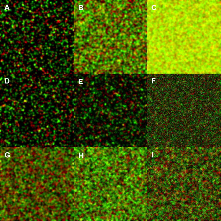
Simulated dual-color images of two interacting species for ICCS analysis, corresponding to a 50% IF. The two-channel images consist of N₀ total particles, N₀/4 are noncolocalized for each color (red and green), and N₀/4 are colocalized particles with each color emitting equal intensity signals for both wavelengths (N₁ = N₂ = N₀/2). The particles are randomly distributed in the image matrix of 256 × 256 pixel image size, and the Gaussian convolution function e⁻² radius was 5 pixels. The first row shows different particle densities with 50% interaction. (A) N₀ = 2 × 10³ (1.2 particles/BA), (B) N₀ = 2 × 10⁴, (C) N₀ = 2 × 10⁵. In the second row, background noise was added to images with N₀ = 2 × 10³ as described in Materials and Methods. (D) S/B = 190, (E) S/B = 14, (F) S/B = 1.7. In the third row, the WF of the counting noise was varied in images with N₀ = 2 × 10⁴. (G) WF = 1, (H) WF = 5, (I) WF = 15.

The first test that was performed to determine the dynamic range of ICCS was to fix the total number of particles in both channels, vary the percentage of interaction, and then repeat for different densities. The minimum interaction percentage required for ICCS to yield a result with a relative error smaller than 10% was calculated as a function of the total particle density of the sample. As the particle density of the sample increases, the minimum measurable IF decreases, improving the dynamic range. When there are just a few particles visible in the image, at least ∼40% of them have to be interacting to obtain an accurate result, but when the density becomes higher than 1 particles/BA, this threshold decreases to ∼¼ of the particles with no upper limit on the particle density. Again, a comparison of the known convolution radius and the radius of the fit Gaussian spatial correlation function is used as the criterion for judging when the analysis had failed. Thus, it is possible to differentiate a priori the correct result by using the convergence of the fitting algorithm instead of having to compare the result obtained with the one set in the simulation, which is of course not feasible in a real experimental situation.

Above this interaction limit of detection, the method yields an accurate result for all IFs and can operate at very high particle densities, with the same proviso regarding the onset of nonideal deviations as was discussed previously for ICS. Even when the density becomes very high, it is still possible to obtain the correct result with accuracy better than 10% (data not shown).

We next set the IF to a value that was shown to be appropriate for the ICCS analysis and then varied the total number of particles in both image channels independently. The result is shown in a contour plot in Fig. 5. It is possible to see that the correct result is only achieved under restricted conditions. The density of particles in each channel cannot be very different; when the ratio between the total numbers of particles of each type is >10, the accuracy decreases dramatically. When this happens, it is not possible to fit the spatial cross-correlation Gaussian function with the proper radius, and it becomes easy to reject the result with confidence. When this ratio becomes larger than one order of magnitude, the relative random overlap between the particles in each channel turns out to be too large to differentiate the central peak from the noise in the correlation function. Nevertheless, it is remarkable that at densities on the order of 1000 particles per BA, ICCS still provides an accurate value for the interaction fraction. The number of particles in the top right corner of Fig. 5 is one order of magnitude larger than the number in the simulated image shown in Fig. 4 C.

FIGURE 5.

Contour plot of the ICCS measured interaction fraction as a function of the densities of particles in both simulated image detection channels. The IF was set to 50% of channel 1 for all the simulations, and the total number of particles was varied independently for both types of particles. The bottom-right black area of the plot corresponds to regimes where the fit of a Gaussian to the spatial cross-correlation function failed and the upper-left black area to densities that cannot exist, given the restriction that 50% of the particles of channel 1 are interacting. The mean result for 50 trials for each set of conditions is plotted. The images consisted of 256 × 256 pixels, and the e⁻² radius of the Gaussian convolving function was set to 5 pixels.

For the simulation of noise, two separate noise matrices were generated for each channel for the two separate cases of background and counting noise, as has been outlined in the Materials and Methods section. Fig. 6 A shows that to obtain an accuracy of at least 10%, the S/B has to be larger than 20 for densities of ∼12 particles per BA per channel and that the S/B has to be greater to obtain accurate results for more dense samples, as was already shown for the single channel images.

FIGURE 6.

(A) Plot of relative error of the IF obtained using ICCS (IF_fit) compared to the IF set in the simulation (IF₀) as a function of the S/B. The mean result of 300 trials for each set of conditions is plotted. The images were 256 × 256 pixels in size, and the e⁻² radius of the Gaussian convolving function was set to 5 pixels. The error bars correspond to the propagation of the SD of the IF recovered by ICCS for each image. (B) Plot of relative error of the IF of particles obtained using ICCS (IF_fit) compared to the IF set in the simulation (IF₀) as a function of the counting noise WF. The mean result for 300 trials for each set of conditions is plotted. The images were 256 × 256 pixels in size, and the e⁻² radius of the Gaussian convolving function was set to 5 pixels. The error bars correspond to the propagation of the SD of the IF recovered by ICCS for each image.

In the case of counting noise, we observe a similar behavior as that for background noise (see Fig. 6 B). For high densities, the counting noise has to be low to achieve acceptable accuracy, but as the density decreases the WF of the signal can increase and still yield similar relative errors. The relative error in the interaction fraction is conceptually different than the number of interacting particles since both the number of interacting particles and the total number of particles is obtained independently from the ICCS analysis.

Spatial ICS on CLSM images of GFP transfected CHO cells

To compare real ICS experiments on cells with the simulations that estimate the accuracy and precision of ICS outlined above, we performed standard CLSM on GFP/EGFR transfected CHO cells. These imaging measurements provide some characteristic numbers related to fluctuation sampling and typical noise levels for the commercial confocal system used.

In Fig. 7, we show a typical CLSM image of a CHO K1 cell expressing GFP/EGFR from which an area 121 × 98 pixels was analyzed using spatial ICS. The experimental e⁻² radius of the PSF is 5.7 pixels, corresponding to a NIF of 116 that yields a relative error of ∼2%. The raw correlation function and its Gaussian fit (Fig. 7 B) are also presented. From the fit amplitude and beam radius, one can calculate a receptor density of 64 μm⁻² (21 particles/BA) after the subtraction of the mean intensity of the background noise distribution.

FIGURE 7.

CLSM image of a CHO K1 cell expressing EGFP/EGFR that was analyzed using spatial ICS. (A) The confocal image of the cell, after mean background subtraction, with the subregion used for spatial ICS analysis outlined in white. (B) Spatial autocorrelation and best fit function calculated for the image region outlined in Fig. 7. The black mesh is the Gaussian function of best fit; the surface is the raw autocorrelation function.

As the boundaries of the cell are clear, it is simple to calculate the mean intensity of the off cell background signal and subtract this value from the whole image before performing the ICS analysis. The SD of the background was calculated as described in Materials and Methods, and together with the average of some of the brightest intensity spots in the image leads to an S/B = 25. Based on the results shown in Fig. 3 A, this value would establish an accuracy of 20% considering only this effect.

It should be noted that we are employing a very conservative approach for background correction in this work. Subtraction of the mean of the background distribution entails a residual contribution of positive background fluctuations (those greater than the mean) to the correlation function, which leads to the systematic error trend depicted in Fig. 5. This approach to background correction would be used in cases where there is no a priori knowledge about the minimum signal level expected. However, in many cases it is possible to apply a higher threshold for background correction and remove more of the background noise distribution. This results in a significant reduction or even elimination of this systematic error in the number density measurement by ICS (depending on S/B ratio). This type of correction is possible in situations where the fluorescent particles of interest are clearly visible above background, such as in the case of resolvable dendritic spines in neurons (23). It is also possible if the minimum fluorescence signal level can be established by imaging a monomeric form of the fluorophore of interest under the same collection conditions as a control (13). Following this approach, a subtraction of the mean plus the SD of the background noise distribution leads to an S/B = 46 and a density of 47 μm⁻² (16 particles/BA) with 10% accuracy.

It is not possible to obtain the WF from just one standard image. To be able to estimate this counting noise factor, 512 × 512 pixel images of 25 mg/ml rhodamine 6G chloride solutions were collected at different laser powers and voltages of the PMT detector. From the intensity histograms of these images, it was possible to compute the WF for our system at the laser intensity used in the cell imaging experiments and this data is shown in Fig. 2S in the Supplementary Material Appendix. The results show that at ∼560V, the WF is so high that the maximum density of the sample at which ICS would yield an accurate and precise result is 100 particles/BA and that the WF would increase for higher PMT voltages. This value is still above the receptor density for many of the cell membrane proteins of interest in normal (nonoverexpressing) cell types. This suggests that in most cases, the noise due to photon detection and collection can be safely neglected for spatial ICS studies. Other experiments with dye solutions at higher PMT voltages yielded WF factors as large as 25 (data not shown).

CONCLUSIONS

We have used simulations to determine the accuracy and precision of spatial ICS and ICCS, given a specified image size, radius of the Gaussian convolution function, and noise levels. Using this information as a guide, it is possible to estimate in advance the accuracy and precision that spatial ICS analysis will yield for a measured number density given specific collection parameters. Furthermore, the simulations for spatial ICCS showed that the interaction fraction in a two-channel dual label study can also be obtained with impressive accuracy for densities typically encountered for membrane receptors.

In the case of ICCS analysis, we have established density and interaction fraction bounds that yield acceptable accuracy and precision. We demonstrated that the NIF is the most important parameter to take into account in terms of statistical sampling, and we have given guidelines to observe when changing the effective sampling through image magnification or image subregion analysis. We have provided estimates of the expected error of the ICS and ICCS methods as a function of the sample particle density and the characteristics of the background and counting noise sources.

We also imaged GFP transfected CHO cells to obtain typical values for the parameters that influence the accuracy and precision of the spatial ICS analysis. Using the CLSM image of a cell and information from control experiments on dye solutions, we could characterize the noise sources and then use the simulation results to estimate the precision of the ICS method. This work presents general results that can be used as a guide for spatial ICS and ICCS experiment design for any arbitrary LSM system.

SUPPLEMENTARY MATERIAL

An online supplement to this article can be found by visiting BJ Online at http://www.biophysj.org.

References

- 1.Magde, D., E. L. Elson, and W. W. Webb. 1972. Thermodynamic fluctuations in a reacting system: measurement by fluorescence correlation spectroscopy. Phys. Rev. Lett. 29:705–708. [Google Scholar]
- 2.Magde, D., E. L. Elson, and W. W. Webb. 1974. Fluorescence correlation spectroscopy. II. An experimental realization. Biopolymers. 13:29–61. [DOI] [PubMed] [Google Scholar]
- 3.Elson, E. L., and D. Magde. 1974. Fluorescence correlation spectroscopy. I. Conceptual basis and theory. Biopolymers. 13:1–27. [DOI] [PubMed] [Google Scholar]
- 4.Magde, D., W. W. Webb, and E. L. Elson. 1978. Fluorescence correlation spectroscopy. III. Uniform translation and laminar flow. Biopolymers. 17:361–376. [Google Scholar]
- 5.Thompson, N. L. 1991. Fluorescence correlation spectroscopy. In Topics in Fluorescence Spectroscopy, Vol. 1: Techniques. J. R. Lakowicz, editor. Plenum Press, New York. 337–378.
- 6.Elson, E. L. 2001. Fluorescence correlation spectroscopy measures molecular transport in cells. Traffic. 2:789–796. [DOI] [PubMed] [Google Scholar]
- 7.Petersen, N. O., P. L. Hoddelius, P. W. Wiseman, O. Seger, and K. E. Magnusson. 1993. Quantitation of membrane receptor distributions by image correlation spectroscopy: concept and application. Biophys. J. 65:1135–1146. [DOI] [PMC free article] [PubMed] [Google Scholar]
- 8.Wiseman, P. W., and N. O. Petersen. 1999. Image correlation spectroscopy. II. Optimization for ultrasensitive detection of preexisting platelet-derived growth factor-beta receptor oligomers on intact cells. Biophys. J. 76:963–977. [DOI] [PMC free article] [PubMed] [Google Scholar]
- 9.Wiseman, P. W., J. A. Squier, M. H. Ellisman, and K. R. Wilson. 2000. Two-photon image correlation spectroscopy and image cross-correlation spectroscopy. J. Microsc. 200:14–25. [DOI] [PubMed] [Google Scholar]
- 10.Brown, C. M., and N. O. Petersen. 1998. An image correlation analysis of the distribution of clathrin associated adaptor protein (AP-2) at the plasma membrane. J. Cell Sci. 111:271–281. [DOI] [PubMed] [Google Scholar]
- 11.Huang, Z., and N. L. Thompson. 1996. Imaging fluorescence correlation spectroscopy: nonuniform IgE distributions on planar membranes. Biophys. J. 70:2001–2007. [DOI] [PMC free article] [PubMed] [Google Scholar]
- 12.Brown, C. M., M. G. Roth, Y. I. Henis, and N. O. Petersen. 1999. An internalization-competent influenza hemagglutinin mutant causes the redistribution of AP-2 to existing coated pits and is colocalized with AP-2 in clathrin free clusters. Biochemistry. 38:15166–15173. [DOI] [PubMed] [Google Scholar]
- 13.Wiseman, P. W., C. M. Brown, D. J. Webb, B. Hebert, N. L. Johnson, J. A. Squier, M. H. Ellisman, and A. R. Horwitz. 2004. Spatial mapping of integrin interactions and dynamics during cell migration by image correlation microscopy. J. Cell Sci. 117:5521–5534. [DOI] [PubMed] [Google Scholar]
- 14.Qian, H. 1990. On the statistics of fluorescence correlation spectroscopy. Biophys. Chem. 38:49–57. [DOI] [PubMed] [Google Scholar]
- 15.Kask, P., R. Günther, and P. Axhausen. 1997. Statistical accuracy in fluorescence fluctuation experiments. Eur. Biophys. J. 25:163–169. [Google Scholar]
- 16.Meseth, U., T. Wohland, R. Rigler, and H. Vogel. 1999. Resolution of fluorescence correlation measurements. Biophys. J. 76:1619–1631. [DOI] [PMC free article] [PubMed] [Google Scholar]
- 17.Wohland, T., R. Rigler, and H. Vogel. 2001. The SD in fluorescence correlation spectroscopy. Biophys. J. 80:2987–2999. [DOI] [PMC free article] [PubMed] [Google Scholar]
- 18.Koppel, D. E. 1974. Statistical accuracy in fluorescence correlation spectroscopy. Phys. Rev. A. 10:1938–1945. [Google Scholar]
- 19.Petersen, N. O. 2001. Spatial correlation spectroscopy. In Fluorescence correlation spectroscopy. R. Rigler and E. S. Elson, editors. Springer Verlag, Berlin Heidelberg. 162–184.
- 20.Brock, R., I. H. L. Hamelers, and T. M. Jovin. 1999. Comparison of fixation protocols for adherent cultured cells applied to a GFP fusion protein of the epidermal growth factor receptor. Cytometry. 35:353–362. [DOI] [PubMed] [Google Scholar]
- 21.Abney, J. R., B. A. Scalettar, and C. R. Hackenbrock. 1990. On the measurement of particle number and mobility in nonideal solutions by fluorescence correlation spectroscopy. Biophys. J. 58:261–265. [DOI] [PMC free article] [PubMed] [Google Scholar]
- 22.Milon, S., R. Hovius, H. Vogel, and T. Wohland. 2003. Factors influencing fluorescence correlation spectroscopy measurements on membranes: simulations and experiments. Chem. Phys. 288:171–186. [Google Scholar]
- 23.Wiseman, P. W., F. Capani, J. A. Squier, and M. E. Martone. 2002. Counting dendritic spines in brain tissue slices by image correlation spectroscopy analysis. J. Microsc. 205:177–186. [DOI] [PubMed] [Google Scholar]
Associated Data
This section collects any data citations, data availability statements, or supplementary materials included in this article.