Modeling Analytical Ultracentrifugation Experiments with an Adaptive Space-Time Finite Element Solution of the Lamm Equation

Abstract

Analytical ultracentrifugation experiments can be accurately modeled with the Lamm equation to obtain sedimentation and diffusion coefficients of the solute. Existing finite element methods for such models can cause artifactual oscillations in the solution close to the endpoints of the concentration gradient, or fail altogether, especially for cases where sω²/D is large. Such failures can currently only be overcome by an increase in the density of the grid points throughout the solution at the expense of increased computational costs. In this article, we present a robust, highly accurate and computationally efficient solution of the Lamm equation based on an adaptive space-time finite element method (ASTFEM). Compared to the widely used finite element method by Claverie and the moving hat method by Schuck, our ASTFEM method is not only more accurate but also free from the oscillation around the cell bottom for any sω²/D without any increase in computational effort. This method is especially superior for cases where large molecules are sedimented at faster rotor speeds, during which sedimentation resolution is highest. We describe the derivation and grid generation for the ASTFEM method, and present a quantitative comparison between this method and the existing solutions.

INTRODUCTION

In recent years, analytical ultracentrifugation has seen a resurgence as a method of choice for characterizing solution behavior of biological macromolecules and macromolecular assemblies. Sophisticated numerical analysis coupled with modern digital data acquisition technology offers a wealth of macromolecular information from this technique. The sedimentation process of a solute in an analytical ultracentrifugation cell is described by the Lamm equation (1),

(1)

where C(r, t) is the concentration, s and D are the sedimentation and diffusion coefficients, and ω is the angular velocity. The terms m and b are the radii of the meniscus and bottom of the cell.

Using a nonlinear least-squares fitting algorithm, data from sedimentation velocity and approach-to-equilibrium experiments can be fitted to finite element solutions of the Lamm equation, and sedimentation and diffusion coefficients, partial concentrations, and to some degree, even equilibrium constants, can be obtained at high resolution. A number of approaches for solving the inverse problem of fitting moving boundary data to finite element solutions of the Lamm equation have been developed and implemented in software packages. Direct fitting of boundary data to fixed-mesh finite element solutions was originally proposed by Claverie et al. (2) and Todd and Haschemeyer (3). In the fixed-mesh approach, radial mesh points are uniformly distributed between the meniscus and the bottom of the cell. Software based on this solution was later developed by Demeler and Saber (4) and Schuck et al. (5). The approach of Stafford and Sherwood (6) fits time-difference data from experimental scans to time-difference data simulated with a fixed-mesh finite element solution. However, the fixed-mesh finite element method suffers from an artifactual broadening of the sedimenting boundary (so-called numerical diffusion). When such solutions are used to fit experimental data, the fitted diffusion coefficients tend to be smaller than the actual diffusion coefficients, especially when the concentration gradient is steep. Later, Schuck introduced an improved finite element solution, the so-called moving hat method (7). This method uses a moving frame of reference and discretizes the Lamm equation under the moving frame by using the standard finite element method. A similar idea relying on distorted grids in finite difference solutions of the Lamm equation has been applied in the earlier developments of sedimentation simulation techniques; see Cox and Dale (8) and references therein. The moving grid employed in the moving hat method is spaced exponentially in the radial direction and shifted at the speed of sedimentation. The moving hat method improves the accuracy of the numerical solution substantially compared to the fixed-mesh approach by Claverie. However, there are two issues not well addressed by the moving hat method. First, even though the gridpoints at the meniscus and at the bottom of the cell have to stay fixed, the moving reference frame used in the moving hat method would require these points to move like all other points in the grid. Therefore, the finite element discretization cannot be applied at the meniscus and at the bottom in the moving hat method. Schuck addressed this singularity by manually adjusting the values of the solution at the bottom and at the point next to the meniscus. Such post-processing is not based on the differential equation itself and may result in loss of accuracy. The second problem with the moving hat method is related to the fact that the grid spacing increases exponentially from the meniscus to the bottom, resulting in low radial mesh point density at the bottom of the cell where concentration changes can be very large, thus lacking the required resolution. It has been pointed out (4,7) that a lack of sufficient radial resolution at the bottom of the solution column results in oscillations in the finite element solution, especially for experimental conditions where sω²/D is large. Such conditions are encountered when large molecules such as DNA molecules >1 kb, multi-enzyme complexes, and large assemblies like chromatin or virus particles are sedimented at moderately high rotor speed. Indeed, if the number of radial mesh points is not large enough, both the Claverie approach and the moving hat method will fail altogether.

Here we present an entirely new finite element method, termed the adaptive space-time finite element method (ASTFEM), for the numerical solution of the Lamm equation that incorporates the advantages introduced by the moving reference frame, and properly addresses the remaining issues in the moving hat method. In this method the Lamm equation is simultaneously discretized in the radial and the time domain (hence the name of space-time finite element method). This space-time discretization avoids the difficulty caused by the singularity of the moving grid at the meniscus and at the bottom in the moving hat method. To eliminate the oscillations around the cell bottom, we implement an adaptive grid locally in a very narrow region next to the cell bottom. The length of this narrow region is proportional to D/(sω²). The number of the grid points placed in the narrow region is ln(sω²/D), which increases very slowly with respect to sω²/D. This fine grid distribution around the cell bottom effectively eliminates the oscillation of the numerical solution. To minimize the numerical diffusion, we use the same moving mesh idea as in Schuck's moving hat method in the region away from the bottom. The length of this region typically ranges between 90 and 99% of the cell length (see below). As a result, the ASTFEM enjoys the same accuracy with respect to numerical diffusion as the moving hat method, but avoids the inaccuracies due to the singularities at the meniscus and bottom of the cell, and completely eliminates oscillations at the bottom of the cell. At the same time the computational costs for all three methods are essentially the same: At each time-step one needs to solve a triangular linear algebraic system of equations with a fixed coefficient matrix. Another important feature of the ASTFEM approach is that the mass conservation of the Lamm equation is guaranteed automatically without the need for any post-processing. Overall, we conclude that the ASTFEM method proposed in this article is an accurate, efficient and robust method for the Lamm equation for sedimentation experiments. Furthermore, the concept of the space-time finite element discretization on adaptive moving grids can be extended to multiple interacting and self-association systems or models with concentration dependent sedimentation and diffusion coefficients.

THE ADAPTIVE SPACE-TIME FINITE ELEMENT SOLUTION OF THE LAMM EQUATION

Let δt represent the size of the time-step, and let t_n = nδt be the n^th time-step. We multiply both sides of the Lamm equation by an arbitrary function v(r, t) and integrate the result over the space-time slab: [m, b] × [t_n, t_n+1]. It follows from integration by parts

(2)

This is called the weak form of the Lamm equation. Any solution to the Lamm equation must satisfy Eq. 2, and any smooth function C(r, t) satisfying Eq. 2 must also be a solution of the Lamm equation. We will derive the finite element solution based on this weak formulation.

To define an approximate solution to Eq. 2, we first divide the space-time slab [m, b] × [t_n, t_n+1] into a number of space-time elements. Each element is either a triangle or a quadrilateral. Let N be the total number of points used in the r-direction, and suppose the grid points r_j, 1 ≤ j ≤ N are already given (see next section for the distribution of the grid points). We connect (r_j, t_n) to (r_j+1, t_n+1) for all j = 1,… ,N – 1. Then the slab [m, b] × [t_n, t_n+1] is divided into N – 1 quadrilaterals and two triangles (one at each end). For each j, let and be the approximate values of C(r, t) at the grid points (r_j, t_n) and (r_j, t_n+1), respectively. We define a continuous function c(r, t) to approximate the exact solution C(r, t) as follows.

Consider a quadrilateral element with vertices (r_j, t_n), (r_j+1, t_n), (r_j+2, t_n+1), (r_j+1, t_n+1). Let be the standard element in an auxiliary ξη-coordinate system. Define the mapping as

(3)

(see Fig. 1). This mapping will be used to introduce the finite element solutions for all r and t on Now, given four values and we define a bilinear function on the standard element as

(4)

FIGURE 1.

Mapping Eq. 3 transforms the standard quadrilateral element into a quadrilateral element The finite element solution on is defined by transforming a bilinear function on with mapping

It follows that takes the values at the four vertices of , respectively. The approximate function c(r, t) on element is defined as the “pull-back” of under the inverse mapping of More precisely, let

be the inverse mapping of Then we define for (r, t) in

and c(r, t) takes the values at the vertices (r_j, t_n), (r_j+1, t_n), (r_j+2, t_n+1), and (r_j+1, t_n+1), respectively.

To define c(r, t) on the triangular element with vertices (r₁, t_n), (r₂, t_n+1), and (r₁, t_n+1), we use the standard triangular element (see Fig. 2). The mapping from to is

(5)

Define a linear function on as

and define the approximate function c(r, t) on as the “pull-back” of the above under the inverse mapping of

FIGURE 2.

Mapping Eq. 5 transforms the standard triangular element into the triangular element The finite element solution on is defined by transforming a linear function on with mapping

Similarly, on the triangular element at the right end of the space-time slab, we can introduce the mapping from to and define the approximate function c(r, t) by the values and

Note that the above piecewise-defined function c(r, t) is continuous on the space-time slab [m, b] × [t_n, t_n+1]. It takes the values and at the vertices (r_j, t_n) and (r_j, t_n+1), respectively, for all j = 1, 2,…,N. Once these values are given, the approximate function c(r, t) is uniquely defined.

Next we introduce a series of test functions v_j(r, t) used in Eq. 2. For each j with 2 ≤ j ≤ N – 1, we define the values of v_j on the grid points as

Then v_j(r, t) is defined piecewise with the above values in the same way as above for c(r, t).

For j = 1 and j = N, we require

and

It is noted that v₁ is non-zero only in For j = 2, 3, …, N, each v_j is only non-zero in the two elements and

Integrals

Given the values of an initial concentration distribution for the approximate solution c(r, t) at time t_n, we now derive a system of linear algebraic equations for the unknown values at the next time-step t_n+1. We ask for the weak form (Eq. 2) to hold for all test functions v_j defined in the last subsection, namely, that the approximate function c(r, t) satisfies

(6)

Since for each j the test function v_j is non-zero only in and (v₁ is non-zero only in ), the above equation can be reduced to

(7)

To evaluate the integrals over we change the variables from (r, t) to (ξ, η) by the mapping from Eq. 3 so that the integrals will be over the standard element The Jacobian J of the coordinate transform is

(8)

where by Eq. 3,

(9)

By the fact that the Jacobian for the inverse transform is equal to the inverse matrix of J, we have

Now it follows from the chain rule of derivatives that

(10)

and by Eq. 4 that

(11)

In addition, note that on that v_j = 1 – ξ. Therefore by putting Eq. 12 into the first term of Eq. 7 we can reduce the integral in

where

For the second integral in Eq. 7, we note the fact that on

Then the second integral in Eq. 7 can be reduced to

where

The third integral in Eq. 7 can be changed into

where

The above formulas cover all the integrals in Eq. 7 over We can deal with the other integrals in Eq. 7 over element similarly. For the two triangular elements at the end of the space-time slab, we need to use the mapping defined in Eq. 5 to change the integrals into those over the standard triangle We skip the details of the formulas, since they can be worked out in the same way as for the quadrilateral elements.

By putting all these integrals into Eq. 6, we obtain a system of linear algebraic equations

(12)

where is the vector of the known approximate values of C at time t_n, and is the vector of the unknown approximate values of C at time t_n+1. M₁ and M₀ are the coefficient matrices assembled from the above integral formulas. Note that both of these two matrices are independent of the time-level n. Therefore, they need to be calculated only once for the entire simulation process. Also, since both M₁ and M₀ are tridiagonal, the system of equations in Eq. 14 can be easily solved. If we use the Gaussian elimination method to solve Eq. 14, then the total number of arithmetic operations needed is only 13N for each time-step. If we perform the LU-decomposition on M₁ (which costs only 5N operations) and store it in memory, then we only need 11N operations at each time-step.

Another important feature of the above ASTFEM scheme is that the mass conservation for the Lamm equation is guaranteed automatically without any post-processing. If we sum up the expressions in Eq. 6 for all j = 1, 2, …, N, and notice that

we have

which implies the conservation of mass

ADAPTIVE GRIDS

In this section we discuss the selection of an ideal distribution of grid points used for the ASTFEM approach described in the last section. First, we recall the behavior of the concentration function C(r, t) in a typical velocity experiment. A notable feature is the rapid buildup of the concentration at the bottom of the cell. This sharp increase can cause numerical oscillations if insufficient radial grid points are used to describe the transition. It is well known that all existing numerical solutions for the Lamm equation, including Claverie's classical finite element method and Schuck's moving hat method, exhibit oscillations at the bottom of the cell if the step size is not small enough. This oscillation happens especially when the sedimentation speed s or angular velocity ω is large or the diffusion coefficient D is small. The oscillations can propagate back toward the meniscus and even cause a complete failure of the computation. Although an increase of the number of grid points will correct this problem, this will also increase the computational cost. Furthermore, a rule to determine an appropriate grid spacing for the fixed-mesh or moving hat method does not exist, and the user is forced to experiment to avoid such oscillations.

Our first aim in the application of adaptive grids is to increase the resolution locally around the cell bottom. The second goal for adaptive grids is to minimize the numerical diffusion typically accompanied with a discretization of sedimentation-diffusion equations. This is essential since numerical diffusion may smooth out the steep boundary of C and predict a larger diffusion coefficient or smaller molecular weight. It is well known in the numerical analysis community (and as observed by Schuck; see (7)) that the numerical diffusion introduced can be greatly reduced by aligning the space-time element with the sedimentation speed (9). Under the moving frame, the Lamm equation is essentially free of numerical diffusion.

Based on this observation, we will define a grid that aligns with the sedimentation speed in most regions of the cell similar to the implementation in the moving hat method. At the same time, we will maintain a very small step size in the narrow region around the bottom. To this end, we divide the interval [m, b] into three different regions: a regular region, a steep region, and a transition region between the steep and regular regions. The grid in the regular region is generated comparable to the grid in the moving hat method. The steep region at the bottom of the cell consists of closely spaced grid elements (the exact spacing is explained below), and the transition region between the two consists of elements whose grid spacing changes gradually from one end to the other to produce a smooth transition of the overall grid spacing.

First we determine the width of the steep region by using the equilibrium condition of the Lamm equation, which is given by

where

We set a threshold C_* of C to indicate the beginning of the steep region. That means we consider [r_*, b] as the steep region with r_* satisfying C(r_*) = C_*. It can be seen that

The reason we choose the equilibrium condition to determine the width of the steep region is that the concentration C(r, t) builds up gradually at the bottom, with the steep region expanding over time. Thus using the equilibrium condition (which corresponds to infinite long time) will include all regions exhibiting a steep concentration change during the entire simulation process.

In our numerical tests we chose C_* = 1/N to slightly increase the steep region for larger N. However, this is not a critical choice. Since C(r, t) is an exponential function of r around the bottom, different C_* values have only a minor effect on the position of r_*, and any other fixed value of C_* will also work well.

Next, we consider the requirement to eliminate the oscillations in the steep region. To avoid oscillations, the grid size δx must be sufficiently small compared to the value of D/(sω²). It is well known that for the discretization of sedimentation-diffusion problems the step size δx should be chosen such that the local Paclet number—which is proportional to the sedimentation speed and the grid size, and inversely proportional to the diffusion coefficient—is smaller than 1 (see Morton (10)). In our case, this condition implies that

(13)

We may simply choose a uniformly distributed grid satisfying Eq. 15 for the steep region. However, noticing that the solution C is exponential as r approaches the bottom b, it is preferable to select a grid that becomes finer and finer as r → b. To this end, we use a simple sine function to determine the grid position in the steep region. We let

be the total number of grid points in the steep region, where ⌊·⌋ represents the integer part of the number in between. We define the grid points in region [r_*, b] as

It follows that the grid size is given by

Therefore, the step size decreases gradually as j increases. The leftmost interval is approximately of size h_*, whereas the rightmost interval is approximately of size which is one order of N_s smaller than h_*.

Next we determine the grid in the regular region. We consider (m, r_°) as the regular region with

The reason to choose r_° as the right end of the regular region is to make the grid size around the right end of the regular region match the grid size around the left-hand side of the transition region. When ν is large, r_° is close to b and most of the cell is regular (see Table 1). The grid points in the regular region are determined analogous to the moving hat method, namely,

where

TABLE 1.

The number of grid points used for the ASTFEM for the simulation of a typical cell with m = 5.8, b = 7.2, and different s, w, and D

		Ns	Nt	Nr	Total	r°	r*
S = 1.562e − 12	N = 101	11	5	99	115	7.169337	7.194758
ω = 50,000 rpm	N = 201	11	4	199	214	7.181502	7.194472
D = 1.279e − 7	N = 1001	13	2	995	1010	7.191381	7.193806
s = 1.0e − 11	N = 101	16	15	99	130	7.176244	7.199993
ω = 60,000 rpm	N = 201	17	14	200	231	7.188469	7.199993
D = 1.0e − 9	N = 1001	18	12	999	1029	7.197067	7.199992

Finally, we determine the grid points in the transition region between r_° and r_*. Let

There are N_t grid points in the transition region,

Note that the step size in the transition region halves from left to right. The length of the rightmost interval in the transition region is h_*, and the length of the leftmost interval in this region is which is approximately the length of the rightmost interval in the regular region.

Since the grid point at the right boundary of the regular region may not match the point at the left boundary in the transition region due to integer rounding in calculating N_t, we need to adjust such that it is positioned halfway in between its two neighboring grid points.

The grid over the entire cell is composed of all the points y_j, t_j, and x_j determined in the above manner. The total number of points actually used is N_s + N_t + N_r. This number is typically a small fraction of N; see Table 1 for the values of N_s, N_t, and N_r for two examples—one with a moderate and one with a very large sω²/D value.

A typical grid defined by the above method is shown in Fig. 3. The nice feature of this mesh is that for most of the region the grid distribution follows the moving frame of reference, which is desirable for maintaining the right sedimentation speed and minimizing the numerical diffusion introduced by discretization. The grids near the cell bottom have a very small step size, which is important to suppress the oscillation and to describe the detailed structure near the bottom of the cell.

FIGURE 3.

ASTFEM grid point distribution for four successive time-steps. A shows the distribution for the entire cell, and in B a zoom of the region near the bottom is shown, clearly identifying the increased density of gridpoints at the bottom of the cell where the change of concentration is the largest and the highest resolution is needed.

Remark

By Taylor's expansion of C(r, t) it is apparent that the discretization error is bigger in regions where the concentration gradient is steep, and the error is small where the solution is relatively flat. To obtain a small overall approximation error, the grid size should be small in regions with large solution curvature, but can be large elsewhere. For a typical concentration function C(r, t) large curvatures do not only exist near the bottom of the cell, but can also exist around the moving boundary. Therefore, an ideal grid distribution should also have higher grid density around the boundary. However, since the solution boundary is moving, this requires adjustment of the grid distribution throughout the simulation, and the coefficient matrices in the linear algebraic system in Eq. 12 need to be recalculated. This will offset the computational savings offered by the adaptive methods. Therefore, we do not consider this option here. However, if the Lamm equation under consideration contains variable sedimentation or diffusion coefficients, then the coefficient matrices require updating at every time-step regardless. In this case, adding the mesh adaptivity throughout the cell does not introduce additional computational work (compared to fixed-mesh methods), and the solution accuracy can be greatly improved.

NUMERICAL RESULTS AND COMPARISON

We compared the accuracy and efficiency of three different finite element approaches for solving the Lamm equation. The first method is the traditional finite element method based on the uniform fixed mesh described by Claverie (2). The second method is the moving hat finite element method developed by Schuck (7). The third approach is the ASTFEM proposed in this work. All three methods essentially utilize the Crank-Nicholson time discretization approach (11). We also examined the effect of the discretization step sizes for space and time and provide some guidelines for choosing the number of grid points for a simulation.

Claverie's finite element method

We first evaluated the finite element method based on a uniform fixed mesh as described by Claverie (2). The time-step sizes are chosen according to the formula given by Schuck (7),

(14)

Our simulation example used the following parameters:

Example 1

(15)

This model approximates a 0.4-kilobase DNA molecule sedimenting through a 7-mm solution column in 1 h. All our simulations were initialized with unity concentration across the entire solution column. We tested four grid densities, N = 101 (δt = 25.90s), 201 (δt = 12.95s), 401 (δt = 6.48s), and 1001 (δt = 2.59s). In Figs. 4–6 we show the numerical solution c(r, t) in different regions and with various N and δt. From these graphs it can be seen that:

1. In the region near the bottom of the cell the oscillation of the numerical solution c(x, t) depends mainly on δx = (b – m)/(N – 1), and not on δt (see Fig. 4).

2. In the region near the meniscus, the oscillation occurs only at the beginning of the simulation. The magnitude of the oscillation depends mainly on the time-step size δt (see Fig. 5). Also, if rotor acceleration is taken into account, the oscillation near the meniscus can be markedly reduced.

3. In the center of the cell, the accuracy of the solution is determined by both N and δt (see Fig. 6).

These observations clearly indicate that, to obtain a highly accurate numerical solution, δx must be very small near the bottom of the cell, and N and δt must be adjusted simultaneously. This is our motivation for the design of the adaptive grids.

FIGURE 4.

Concentrations c(r, t) around the cell bottom obtained by Claverie's finite element method using (A) different numbers of grid points but the same time-step size, and (B) different time-step sizes but the same number of grid points. The parameters for this experiment are from Example 1, and t = 4922 s. From this figure it can be seen that the occurrence of oscillations at the bottom of the cell is strongly dependent on radial grid spacing, whereas a change of the time spacing has little influence.

FIGURE 5.

Concentrations c(r, t) around the meniscus obtained by Claverie's finite element method using (A) different numbers of grid points but the same time-step size, and (B) different time-step sizes but the same number of grid points. The parameters for this experiment are from Example 1, and t = 25.9, 77.7, and 129.5 s. Here, the result is opposite to the effect shown in Fig. 4, and the oscillations near the meniscus are mostly influenced by the time discretization and only exist for the first several time-steps. Further reduction in the oscillation can be achieved by taking into account the rotor acceleration period at the beginning of the run.

FIGURE 6.

Concentrations c(r, t) boundaries around the middle of the cell obtained by Claverie's finite element method using (A) different numbers of grid points but the same time-step size, and (B) different time-step sizes but the same number of grid points. The parameters for this experiment are from Example 1, and t = 518.0 s. In the middle of the cell the solution accuracy is affected by both the time and radial step size.

Schuck's moving hat method

Next, we evaluate the performance of Schuck's moving hat method. The grid for time level t_n used in the moving hat method is given by

(16)

The same grid is used for the next time-step t_n+1, but the entire grid is shifted right by one point, with the last point deleted. See Fig. 7 for a typical grid used in the moving hat method. The basic idea in the moving hat method is first to introduce a time-dependent coordinate transform r′ = r′(r, t) and change the Lamm equation into a differential equation in (r′, t)-variables, and then to discretize this equation with the standard finite element method. The exponential grid distribution from Eq. 16 sets the grid-speed equal to that of the sedimentation speed. In this case, the Lamm equation is free of sedimentation under the moving coordinate system. There are two issues not well addressed by the moving hat method:

1. The step size δx determined by Eq. 16 is too large around the cell bottom (even larger than in the rest of the cell), although a smaller step size is actually necessary for this region to accurately resolve the exponential buildup of the concentration. Therefore, the numerical solution by the moving hat method exhibits oscillations around the cell bottom if N is not sufficiently large (see Figs. 8 and 9, A, C, and E).

2. The coordinate transform used in the moving hat method is singular at the meniscus and at the bottom. This is because at these points the grid is required to move according to the sedimentation velocity, even though these positions are fixed and have to remain at the meniscus and at the bottom. Therefore, the finite element discretization cannot be applied to the two points at the meniscus and the bottom.

FIGURE 7.

A typical grid used in the moving hat method for four successive time-steps. The radial distribution of the grid points is determined according to Eq. 16. The grid point density decreases toward the bottom of the cell, with the largest spacing at the bottom of the cell, where the highest resolution is actually needed.

FIGURE 8.

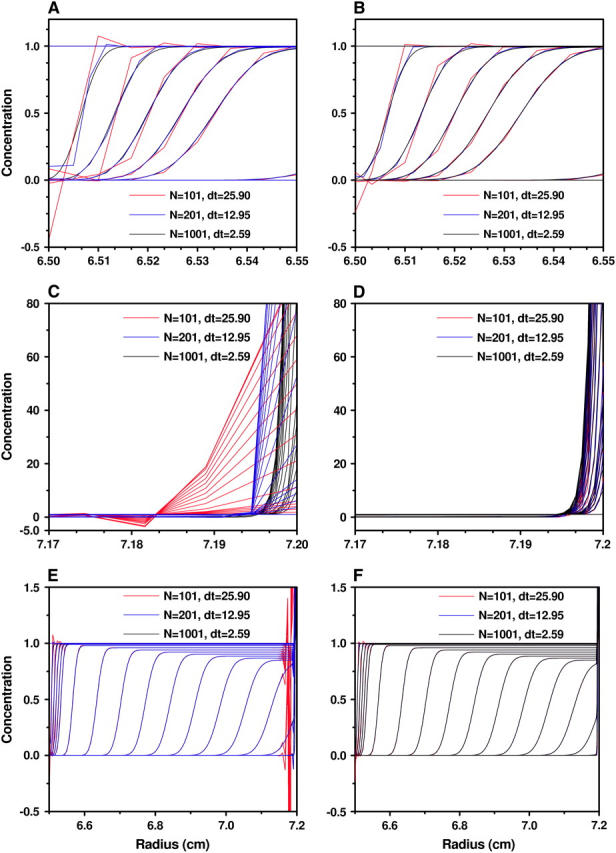
Concentrations obtained by the moving hat method (A, C, and E) and the ASTFEM method (B, D, and F) with various N and δt for Example 1 (m = 6.5 cm, b = 7.2 cm, s = 10⁻¹², D = 2 × 10⁻⁷, 60,000 rpm, 9000 s). (A and B) The concentrations near the meniscus. (C and D) The concentrations near the bottom of the cell. (E and F) The concentrations on the entire cell. The largest difference can be noticed at the bottom of the cell (C and D), where the moving hat method is poorly conditioned. The oscillations near the meniscus are reduced for the ASTFEM method (A and B), and can be significantly reduced for both solutions when slow rotor acceleration is modeled in the solution.

FIGURE 9.

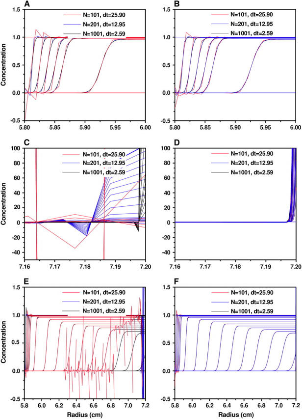
Concentrations obtained by the moving hat method (A, C, and E) and the ASTFEM method (B, D, and F) with various N and δt for Example 2 (m = 5.8 cm, b = 7.2 cm, s = 1.562 × 10⁻¹², D = 1.279 × 10⁻⁷, 50,000 rpm, 6000 s). (A and B) The concentrations near the meniscus. (C and D) The concentrations near the bottom of the cell. (E and F) The concentrations on the entire cell.

Schuck dealt with this problem by imposing two additional conditions:

1. The value is the weighted average of and

2. The value is determined by requiring that the total mass at t_n+1 is equal to that at t_n.

Although these two conditions are consistent with the continuous equation, they are not based directly on the finite element discretization, i.e., they are a type of post-processing, whose effect is not determined by the properties of the Lamm equation. Nevertheless, the moving hat method is much more accurate than the fixed grid finite element method, even though it does not fix the oscillation problems near the bottom of the cell associated with the standard method by Claverie.

Comparison of ASTFEM with the moving hat method

Next, we evaluated the performance of the ASTFEM method based on the adaptive grid solution described earlier, and compared it to the moving hat method. Since the moving hat method is much more accurate than the standard finite element method by Claverie et al. (2), we do not present the comparison with the fixed-mesh method.

To illustrate the difference between the two methods we chose the following experimental conditions corresponding to a 1-kilobase DNA molecule in random coil conformation sedimenting in a 1.4-cm column over 1.5 h:

Example 2

(17)

In this case, the time-step was calculated according to Eq. 16 to be δt = 50.49 for N = 101 points. In Figs. 8 and 9 we plot the numerical solution obtained from the moving hat method and the ASTFEM method with various N and δt. We observe from these figures that:

1. For the moving hat method, if N is sufficiently large (e.g., N ≥ 400 for Example 1, above), the oscillation around the bottom can be eliminated, and the solution is quite accurate. When N is moderate, the oscillation occurs around the bottom, and it does not propagate back into the cell by much. But the buildup of the concentration at the cell bottom has been considerably broadened (Figs. 8 C and 9 C), and the accuracy in the bottom region is very poor. When N is small, e.g., N = 100 for Example 2, the oscillation can travel back rapidly toward the meniscus of the cell and destroy the solution profile completely.

2. For the ASTFEM method, the solutions are not only very well resolved around the bottom, but also maintain a high accuracy around the boundary at all times. Most importantly, they are free from oscillation around the cell bottom for both examples with N = 100. We even tested some unrealistic cases with D = 10⁻¹⁴ and N = 100 and found no oscillation at the cell bottom, and the solution remains highly accurate. Thus, unlike the moving hat method, the ASTFEM solution with the adaptive grids proposed in this article never breaks down and is extremely robust. The issue of conservation of mass is also handled remarkably well by ASTFEM. Even for a small number of grid points the method maintains the total mass within no less than seven-decimal-digits accuracy without any post-processing during the entire simulation.

To compare the two methods quantitatively, we choose as the reference solution a numerical solution obtained using Claverie's fixed-mesh finite element method with a very large number of radial grid points and a very small δt (N = 10⁴ and δt = 0.259 for Example 1, and N = 10⁴ and δt = 5.049 for Example 2). Then we measure the difference between the moving hat or ASTFEM solutions and the reference solution. Since in all experimental data analysis the data near the meniscus and near the bottom of the cell are excluded from the fit, we consider here only data points from the solution column that are slightly inside the meniscus and the bottom of the cell, and calculate only the errors between two internal points r_a and r_b in the cell. We choose r_a = m + 0.05(b − m) and r_b = b – 0.05(b − m), which means that 5% of the solution column next to the meniscus and the bottom are excluded from the accuracy check. For the comparison, we calculate for each time-step t the maximum error

and the L² error (which is equivalent to the square-root-mean error in the discrete case)

We plot in Fig. 10 the errors versus time t for different numerical methods. From these results we observe that both ASTFEM and the moving hat method (when it is convergent) exhibit second-order convergence properties (12), i.e., if the step size δx and δt are reduced by a factor of 2, the error is reduced by a factor of 4. With about the same number of grid points, ASTFEM is always more accurate than the moving hat method. In particular, when D is small, the moving hat method fails altogether, but ASTFEM remains quite accurate. If we include the entire cell from meniscus to bottom for the error comparison, then ASTFEM is much more accurate than the moving hat method, since the latter cannot resolve the solution sufficiently at the bottom.

FIGURE 10.

Comparison of the evolution of the errors between the reference solution and the moving hat solutions or the ASTFEM solutions. (A and C) The L² error and the maximum error for the experiment setting in Example 1. (B and D) The L² error and the maximum error for the experiment setting in Example 2. Note that the ASTFEM solution achieves a lower error for all cases, and unlike the moving hat method, for N = 100 the ASTFEM solution remains stable and accurate.

Guideline for choosing N

A practical question in the numerical solution of the Lamm equation is how many grid points one should use to get a sufficiently accurate approximate solution. A satisfactory answer to this question clearly depends on the following factors: the measure of what constitutes an acceptable error, the portion of the solution column to be included for the finite element fit of the experimental data, and the parameters for the Lamm equation. For our error comparison we consider here the L²-norm, and include only 90% of the solution column in middle for the accuracy check, and report on the dependence of the accuracy on N, s, D, and ω.

First, it is clear that the effects of s and ω are not independent of each other. It is the product of sω² which determines the behavior of the solution of the Lamm equation. Therefore, we fix the rotor speed at 50,000 rpm, and examine the effects of various values of s.

Here we consider two scenarios, the first is for a fixed D and a varied s, and the second is for a fixed s and a varied D. In Fig. 11 we plot the L² error versus time for various sedimentation coefficients. Note that for different sedimentation coefficients the total time needed to reach the equilibrium state is different. Hence the error curves dip at different times. Furthermore, it can be seen from Fig. 11 that for different s, the accuracy is different mainly at the beginning of the process. Once the solution profile is established, the solution accuracy is almost the same for different s. This can be explained by the fact that the Lamm equation is sedimentation-free under the moving computation grids. Therefore, the solution accuracy is almost independent of the sedimentation coefficient.

FIGURE 11.

The evolution of the L²-error in time for the ASTFEM solutions using N = 101 and 201 for experiments of various sedimentation coefficient s. Here the rotor speed was simulated at 50,000 rpm, D = 10⁻⁷, and m = 5.8, b = 7.2. This graph indicates that the accuracy of an ASTFEM solution does not depend much on the s values when the concentration boundary is in steady propagation. The same conclusion is true for Claverie's solution and the moving hat solution.

To examine the accuracy with respect to the diffusion coefficient D, we average the L² error at each time-step t to get an averaged global L² error. More precisely, we consider

where T is the duration of the experiment. The square of this measure is equivalent to the variance for the samples consisting of all the c(r_j, t_n) values. In Fig. 12 we plot the averaged L² error versus the reciprocal of the square root of the diffusion coefficient. This graph indicates a linear relationship between the error and

FIGURE 12.

The averaged L²-error |c – c_ref| versus of the ASTFEM solution for experiments of various diffusion coefficient D. Here the rotor speed was simulated at 50,000 rpm, s = 10⁻¹², and m = 5.8, b = 7.2. This graph indicates that the accuracy of an ASTFEM solution increases as the diffusion coefficient D increases. The same conclusion is also true for Claverie's solution and the moving hat solution.

Combining the above observations, we conclude that away from the meniscus and the bottom the error of the ASTFEM solution is roughly a linear function of and a quadratic function of 1/N, and independent of s or ω, i.e.,

(18)

In practice, one may estimate the error by using the Richardson extrapolation technique. More precisely, start with a small N, say N = 100. Compute the ASTFEM solution using N points. Then compute another ASTFEM solution using 2N points, and by Eq. 18 we have

Hence we have from the triangle inequality that

which implies

This can predict quite accurately the range of the actual error. Listed in Table 2 is the comparison of the actual error against a reference solution (obtained by using 1001 points), and the difference |c_N – c_2N| for N = 101. Clearly this extrapolation technique can be used to get an estimate of the actual error and determine a proper N.

TABLE 2.

The actual error ∥c_N − c_ref∥ and the difference of two numerical solutions ∥c_N − c_2N∥ for the case m = 5.8, b = 7.2, s = 1e – 12, 50,000 rpm, and N = 101

	D = 1e − 7	D = 2e − 7	D = 4e − 7	D = 8e − 7
∥cN – cref∥	1.01579e − 03	6.54426e − 04	4.36885e − 04	2.99125e − 04
∥cN – c2N∥	1.00326e − 03	6.63717e − 04	4.51976e − 04	3.17079e − 04

CONCLUSION AND DISCUSSIONS

In the previous sections we studied the behavior of three numerical solutions of the Lamm equation, and proposed an adaptive space-time finite element solution method. The features of this ASTFEM approach include:

1. It is free from the oscillation typically observed at the bottom of the cell with Claverie's finite element method and Schuck's moving hat method in experiments with large molecules and/or high rotor speed. Indeed, there is no observable oscillation for the ASTFEM solution with only ∼100 points for any experimental parameter combination we have tried, suggesting that the ASTFEM solution provides superior robustness.

2. ASTFEM is much more accurate than Claverie's fixed-mesh or Schuck's moving hat method in the region near the cell bottom. It is also always more accurate than these two methods in the other regions of the cell.

3. ASTFEM automatically guarantees mass conservation of the Lamm equation without any post-processing.

4. The computational cost of ASTFEM is the same as for Claverie's and Schuck's method. All of them need to solve a tridiagonal linear system of equations with a fixed coefficient matrix for each time-step. Therefore, we conclude that ASTFEM is superior to both Claverie's and Schuck's methods.

The significance of the improvements in accuracy and concomitant efficiency are important for several reasons. The numerical solution of the Lamm equation by finite element methods is computationally relatively expensive. Nonlinear least-squares fitting of experimental sedimentation data with such solutions is an iterative process that often requires many repetitions of function evaluations. Statistical analysis of fitting results with Monte Carlo requires several thousand evaluations. Thus, improvements in efficiency are amplified in fitting applications and statistical analysis. In addition, the robustness displayed by the ASTFEM method is important for the stability of unconstrained fitting sessions where parameters may assume values under which the moving hat or fixed-mesh method will simply fail, but ASTFEM solutions will remain well-conditioned.

The idea of space-time finite element discretization can be extended directly to the cases of interacting and self-association systems, and cases for concentration dependency of s and D. One of the advantages of the ASTFEM approach is that the mass conservation is satisfied automatically in these cases. We will report the numerical solution and results for interacting and concentration-dependent solutes in a forthcoming publication.

It is noted that we only attempted to use adaptivity around the cell bottom. Mesh adaptation to the concentration boundary would require the update of the coefficient matrix of the linear system, which increases the computational work substantially. However, for cases where the diffusion or sedimentation coefficients are dependent on the concentration itself, the coefficient matrix needs to be updated from time to time anyway, and then such adaptation will not introduce additional work to the solution procedure. This is a topic under current investigation.

References

- 1.Lamm, O. 1929. The differential equation of the ultracentrifuge. Ark. Mat. Astron. Fys. 21B:1–4. [Google Scholar]
- 2.Claverie, J.-M., H. Dreux, and R. Cohen. 1975. Sedimentation of generalized systems of interacting particles. I. Solutions of systems of complete Lamm equations. Biopolymers. 14:1685–1700. [DOI] [PubMed] [Google Scholar]
- 3.Todd, G. P., and R. H. Haschemeyer. 1981. General solution to the inverse problem of the differential equation of the ultracentrifuge. Proc. Natl. Acad. Sci. USA. 78–11:6739–6743. [DOI] [PMC free article] [PubMed] [Google Scholar]
- 4.Demeler, B., and H. Saber. 1998. Determination of molecular parameters by fitting sedimentation data to finite-element solutions of the Lamm equation. Biophys. J. 74–1:444–454. [DOI] [PMC free article] [PubMed] [Google Scholar]
- 5.Schuck, P., C. E. MacPhee, and G. J. Howlett. 1998. Determination of sedimentation coefficients for small proteins. Biophys. J. 74–1:466–474. [DOI] [PMC free article] [PubMed] [Google Scholar]
- 6.Stafford, W. F., and P. J. Sherwood. 2004. Analysis of heterologous interacting systems by sedimentation velocity: curve fitting algorithms for estimation of sedimentation coefficients, equilibrium and kinetic constants. Biophys. Chem. 108:231–243. [DOI] [PubMed] [Google Scholar]
- 7.Schuck, P. 1998. Sedimentation analysis of noninteracting and self-associating solutes using numerical solutions to the Lamm equation. Biophys. J. 75–3:1503–1512. [DOI] [PMC free article] [PubMed] [Google Scholar]
- 8.Cox, D. J., and R. S. Dale. 1981. Simulation of transport experiments for interacting systems. In Protein-Protein Interactions. C. Frieden and L.W. Nichol, editors. Wiley, New York. 173–211.
- 9.Varoğlu, E., and W. D. L. Finn. 1980. Space-time finite elements incorporating characteristics for the Burgers equation. Int. J. Num. Methods Eng. 16:171–184. [Google Scholar]
- 10.Morton, K. W. 1996. Numerical Solution of Convection-Diffusion Problems. Chapman & Hall, London.
- 11.Crank, J., and P. Nicholson. 1947. A practical method for numerical evaluation of solutions of partial differential equations of the heat conduction type. Proc. Cambridge Philos. Soc. 43:50–67. [Google Scholar]
- 12.Bank, R. E., and R. F. Santos. 1993. Analysis of some moving space-time finite element methods. SIAM J. Num. Anal. 30:1–18. [Google Scholar]
- 13.Demeler, B. 2005. The UltraScan Software Package—a comprehensive data analysis package for sedimentation experiments. Http://www.ultrascan.uthscsa.edu.