Observation Volumes and γ-Factors in Two-Photon Fluorescence Fluctuation Spectroscopy

Abstract

Fluorescence fluctuation spectroscopy has become an important measurement tool for investigating molecular dynamics, molecular interactions, and chemical kinetics in biological systems. Although the basic theory of fluctuation spectroscopy is well established, it is not widely recognized that saturation of the fluorescence excitation can dramatically alter the size and profile of the fluorescence observation volume from which fluorescence fluctuations are measured, even at relatively modest excitation levels. A precise model for these changes is needed for accurate analysis and interpretation of fluctuation spectroscopy data. We here introduce a combined analytical and computational approach to characterize the observation volume under saturating conditions and demonstrate how the variation in the volume is important in two-photon fluorescence correlation spectroscopy. We introduce a simple approach for analysis of fluorescence correlation spectroscopy data that can fully account for the effects of saturation, and demonstrate its success for characterizing the observed changes in both the amplitude and relaxation timescale of measured correlation curves. We also discuss how a quantitative model for the observed phenomena may be of broader importance in fluorescence fluctuation spectroscopy.

INTRODUCTION

Fluorescence correlation spectroscopy (FCS) and related fluctuation spectroscopy methods such as photon-counting histograms and fluorescence intensity distribution analysis are gaining widespread use due to their important capabilities for characterizing the chemical and physical properties of experimental systems at the single molecule level (1–3). This includes the capability to measure the mobility, interactions, chemical kinetics, and physical dynamics of biomolecules both in vitro and in vivo (4–9). The basic strategy of fluctuation spectroscopy experiments is to apply statistical analysis tools to analyze the fluctuations in measured fluorescence intensity from a minute sample observation volume (10). The open observation volume is optically defined using either two-photon or confocal microscopy, and information recovery from fluctuation experiments requires an accurate characterization and calibration of the size and shape of the observation volume. Simple models for the profile of the observation volume are routinely applied to derive curve-fitting functions, and both three-dimensional-Gaussian (3DG) and Gaussian-Lorentzian (GL) models of the observation volume are used with good success to analyze fluctuation data (11–13). However, it is not widely recognized that the measurement volume can be highly dependent on the underlying physics of the fluorescence measurement process, particularly on the fluorescence excitation parameters (14). Although the simple 3DG and GL models can be used to fit individual fluctuation data sets when there is no variation in excitation parameters across that data set, the models are quite inadequate to account for measurements over a broad range of excitation conditions (15). For example, the simple models cannot be used to analyze fluctuation data acquired over a range of excitation powers or for fluorescent molecules with substantially different absorption cross-sections without a corresponding unphysical variation in the recovered fitting parameters. Moreover, the recovered fitting parameters are not always physically meaningful, which can further complicate data analysis procedures. These problems have several important implications for the design and analysis of fluctuation measurements, as will be discussed below.

It is therefore highly desirable to develop accurate models for the observation volume that can quantitatively describe observed fluorescence fluctuation data even when there are variations in excitation conditions. As we have recently demonstrated, the main reason the simple 3DG and GL models fail to accurately fit data acquired under different excitation conditions is that excitation saturation leads to important changes in the size and profile of the observation volume (15). As a first attempt to account for the volume changes quantitatively, we introduced a phenomenological model to describe the saturation-modified volume. Although this model could account for some of the observed variations in FCS measurements, it was rather limited in the range of excitation conditions it could accurately describe. This left a need for a more precise characterization of the observation volume and its effects on fluctuation spectroscopy measurements, preferably based on the underlying physics of the excitation saturation process rather than a phenomenological treatment. For a given focused laser excitation profile, a precise and physically accurate representation of the true observation volume is relatively straightforward to compute (14,16). We here demonstrate how the modified observation volumes are important for fluctuation spectroscopy. We begin with a brief introduction of how fluorescence observation volumes and γ-factors are defined in two-photon microscopy, and their relevance to fluctuation measurements. We then provide a quantitative description of the total volume and the γ-factors for the fluorescent observation volumes under varied excitation conditions, showing computationally how saturation-induced volume variations influence FCS curve amplitudes and relaxation timescales. We then introduce a simple modification to standard curve-fitting procedures that allows for full and accurate characterization of observation volumes over a wide range of molecular excitation rates, and we demonstrate its effectiveness for fitting FCS data. Although the general phenomena discussed here are highly relevant to all forms of fluctuation spectroscopy, we will, for simplicity, restrict the discussion specifically to FCS measurements, and focus exclusively on two-photon FCS measurements.

Background

Two-photon fluorescence signals, observation volumes, and γ-factors

The basic theory of two-photon excited fluorescence has been widely reported (17,18). The instantaneous rate for absorption of photon pairs follows the familiar intensity-squared dependence, and is given by 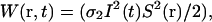where σ₂ is the two-photon absorption cross-section, I(t) is the laser flux (in photons/cm²/s) at the center of the focused two-photon excitation source, and S(r) is a dimensionless distribution function representing the three-dimensional spatial profile or point-spread function (PSF) of the focused laser excitation. For most fluctuation spectroscopy applications one is interested in measured fluctuations on timescales that are much longer than the laser pulse width and pulse repetition rate. Therefore, it is convenient to work with the time-average excitation rate, determined by integrating W(r,t) over a single laser pulse to find the total molecular excitation probability per pulse, and multiplying the result by the laser pulse repetition rate. Specifically, the average excitation rate can be written as where the angular brackets represent the time average. (The temporal profile of the laser pulses must be specified to compute this average; see Ref. 18 for details.)

Without saturation, the measured fluorescence signal from a unit volume at any point in space is directly proportional to the average molecular excitation rate multiplied by the local molecular concentration, C(r,t). On can therefore express the rate that fluorescence photons are measured from a unit volume as κ〈W(r)〉C(r,t), where the factor κ accounts for the fluorescence quantum yield and the detection efficiency of the instrumentation. The total measured fluorescence signal is determined by adding up the signal from all regions of the sample, and can be expressed as

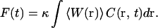(1)

We note that the above integral is evaluated over all space, and that the physical volume represented by the limits of integration is essentially infinite, limited only by the sample container walls. This raises the question of what quantity is most appropriately used to specify the fluorescence observation volume. In fact, there is no explicit measurement “volume” in the traditional sense of the word, in that there is no physical boundary that designates whether or not molecules reside within or outside of what is generally referred to as the “observation volume”.

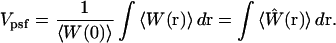
However, one can construct a volumelike quantity, based on the optically defined molecular excitation rate profile, which provides a useful tool for estimating the approximate size of the physical region from which the majority of the measured fluorescence is generated. This is accomplished by dividing the total fluorescence signal of Eq. 1 by the fluorescence-per-unit-volume generated by molecules located at the center of the focused laser beam. In other words, the volume is specified by the integral of the distribution function describing the relative probability of generating fluorescence photons at various spatial locations within the laser PSF, normalized to the probability for generating photons at the center of the excitation beam. Specifically, the measurement volume is defined as

(2)

In this notation, 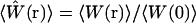is the normalized fluorescence excitation probability that defines the profile of the observation volume. This definition of volume provides a very convenient notation for discussing fluorescence fluctuation measurements, although it is helpful to remember that this volume represents a normalized probability rather than a container size. The actual size of the sample region that makes significant contributions to the measured fluorescence signal will be larger than the volume calculated by Eq. 2. As will be shown below, it is the probabilistic nature of the volume definition that leads to significant alterations in the size and profile of the observation volume under different excitation conditions.

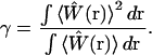
Due to the probabilistically defined volume, V_psf is not in itself fully sufficient to characterize the observation volume. Higher order moments of the distribution function that defines the volume are also important for modeling fluctuation spectroscopy measurements. In the context of FCS and related fluorescence correlation techniques, the additional required parameter is referred to as the γ-factor (19,20). This parameter is a measure of the uniformity of the fluorescence signal from molecules located at various locations within the volume and the effective steepness of the boundary defining the volume, and is defined as

(3)

For the optically defined volumes characteristic of two-photon or confocal microscopy, the γ-factor always has a value <1. A value of unity (γ = 1) is obtained only when the volume has well-defined physical boundaries characteristic of a physical container and the fluorescence signal from individual molecules is the same for molecules located in all regions of the volume. We note that some authors prefer to incorporate the γ-factor into their definition of the “volume,” defining an effective detection volume as 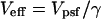(12,21,22). In this manuscript we use volume to refer to V_psf, as defined in Eq. 2.

With the above definitions for the volume, together with Eq. 1, the average measured fluorescence signal can be written conveniently as 〈F〉 = ψ〈C〉V_psf. Here we have introduced the molecular brightness parameter, ψ = κ〈W(0)〉, which depends explicitly on the excitation conditions and specifies the average number of fluorescence photons per molecule per second measured from molecules located in the center and at the focal plane of excitation laser. The molecular brightness is one of the most important parameters in fluctuation spectroscopy measurements (23). The expression for the total fluorescence is sometimes further simplified as 〈F〉 = ψN, where N is calculated by multiplying the concentration by the volume. The value of N is typically referred to as the “number of molecules” within the volume, although this expression should not be interpreted literally. The actual number of molecules that contribute to the total measured fluorescence signal will be larger than the value N. We note that the discrepancy between the value N and the actual number of molecules making a contribution to the fluorescence signal exists regardless of which definition of the volume is preferred. To clarify possible confusion on this point, we note that the expression 〈F〉 = ψ〈C〉V_psf = ψN is mathematically identical to Eq. 1, and thus rigorously accounts for the variation in measured fluorescence signals from molecules located in different regions of the observation volume. However, to correctly interpret this simplified expression for the total measured fluorescence signal one needs always to consider that V represents a probabilistically defined open volume rather than a physically closed volume, and that this expression does not imply that all molecules within different physical regions of the laser excitation all generate equivalent fluorescent signals. In other words, the statement that there are specifically N molecules within the volume each contributing ψ photons per second yields a numerically correct value for the total measured fluorescence signal, but a conceptually inaccurate representation of the actual fluorescence measurement. The total fluorescence signal arises from a larger sample volume and larger number of molecules than the values V_psf and N represent, and molecules in the periphery of the beam contribute fewer than ψ photons per second to the measured signal.

Fluorescence correlation spectroscopy

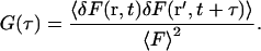
In fluctuation spectroscopy, measured fluorescence fluctuations serve as reporters of local concentration fluctuations within the observation volume, which can originate from various underlying causes such as diffusion, chemical kinetics, conformational dynamics, or photophysics (10,19). Concentration in this context should be interpreted broadly, representing the concentration of particular fluorescent entities. Chemical or physical dynamics that result in altered molecular states or fluorescent properties are in this context also regarded as concentration fluctuations. The fluctuation dynamics are thus all contained within the concentration term in Eq. 1. The fluorescence fluctuations are therefore typically written as 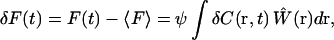where 〈F〉 represents the time-averaged fluorescence intensity, and δC(r,t) the local concentration fluctuations. In FCS, the experimental system dynamics are analyzed by calculating the correlation function of the measured fluctuations, defined as

(4)

With an appropriate model for the underlying physical and chemical fluctuation dynamics, one can solve for explicit representation of the correlation function. For example, for purely diffusive systems, FCS curves are most commonly analyzed using an equation for the correlation function derived for the 3DG observation profile. (The 3DG profile is defined as with 1/e² beam waists ω₀ and z₀, and V_3DG represents the V_psf for the 3DG profile; see Refs. 11 and 24.) For two-photon excitation with diffusion coefficient D, the corresponding correlation function is found to be

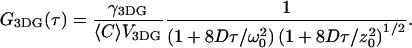(5)

We note that this solution is sometimes written in terms of the diffusion time, defined as 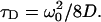The diffusion time is related to the average time a molecule will reside within the observation volume before diffusing out. Although the exact mathematical form of the correlation function depends on the profile of the observation volume as well as the underlying physical dynamics, it is in general possible to represent the normalized correlation function as

(6)

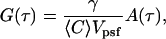
where 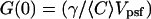represents the amplitude of the correlation function and A(τ) represents the temporal relaxation profile (A(0) = 1). We note that the amplitude of the correlation function is also often written as 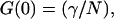where again N represents the product of the volume and concentration as defined above. When the γ-factor is incorporated into the volume definition as discussed above, the correlation amplitude is written simply as 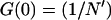(21). In this expression, the number of molecules, N′, is related to the number defined above as Mathematically, both definitions of the volume and number of molecules produce equivalent results in FCS analysis, although the differing notation has led to some confusion in the literature. In this article, we will continue to work with the volume as defined in Eq. 2, and to avoid further confusion, use explicit concentration-dependence instead of referring to the number of molecules.

Excitation saturation

As noted above, the fluorescence signal increases linearly with increasing two-photon absorption rates, and thus quadratically, with the excitation intensity in the absence of excitation saturation. The profile of the observation volume, defined by is therefore completely determined by S²(r), the square of the focused laser PSF. On the other hand, as the fraction of molecules excited during each laser pulse increases toward unity, the effective molecular excitation rate becomes limited by excitation saturation. This well-known phenomenon is caused by both ground state depletion and stimulated emission, and with saturation the average fluorescence excitation rate no longer varies linearly with the two-photon absorption rate (25). This leads to a breakdown in the quadratic dependence of the overall fluorescence signal on excitation power. Moreover, since molecules at different locations within the focused laser profile experience different excitation rates, the degree of saturation also varies throughout the observation volume with molecules at the center of the beam experiencing a greater degree of saturation than those on the periphery. Thus, once saturation effects become significant, further increases in the excitation rate will increase the fluorescence signal from molecules in the periphery of the beam more than those in the center of the beam. Keeping in mind that the observation volume is specified entirely by the relative probabilities for fluorescence excitation at various regions within the PSF, it is immediately apparent that saturation effects will lead to a change in the size and shape of the volume.

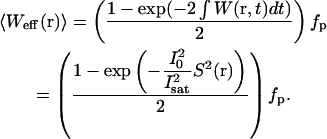
To quantitatively model the effective fluorescence excitation rates, observation volume, and γ-factors under saturating conditions, one must solve the rate equations describing the fluorescent molecular system. A simple two-state model is sufficient to capture the important saturation dynamics. Finding a solution for the ground and excited-state molecular populations using this two-state model is complicated by the pulsed nature of two-photon excitation, since one is interested in the transient excited-state population after each laser pulse, rather than a steady-state solution. In general, the equations must be solved numerically (14). However, in the limit where the laser pulses are much shorter than the fluorescence lifetime—a condition that is typically met in two-photon microscopy—the rate equations have a simple analytical solution. The solution specifies the average effective fluorescence excitation rate, 〈W_eff(r)〉, in terms of the instantaneous two-photon absorption rates, W(r,t), and is written as

(7)

Here f_p is the laser pulse repetition rate and the integral in the exponential is again evaluated over a single pulse. The quantity I₀ represents the peak illumination intensity, and I_sat will be referred to as the saturation intensity. The precise definition of the saturation intensity depends explicitly on the temporal profile of the pulsed excitation. For a square temporal profile the saturation intensity is defined in terms of the fundamental system parameters as where α is the laser pulse width. For more realistic temporal pulse profiles this expression for the saturation intensity would have the same dependence on the two-photon absorption cross-section and pulse width, but also be multiplied by a constant of order unity that arises from the integral in the exponent of Eq. 7. For Gaussian-shaped pulses, this constant has the value 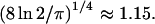This constant is of little practical importance for our current purposes, since I_sat will generally be used as a fitting parameter in data analysis routines. Regardless of the pulse shape, the saturation intensity corresponds to the excitation intensity, for which half of the molecules at the center of the volume would be excited by each laser pulse, if saturation did not alter the quadratic dependence of the fluorescence excitation rate on laser flux.

It is important to note that the effects of excitation saturation become important at excitation intensities below the saturation intensity. As shown in the next section, at the saturation intensity the effective volume has already increased by ∼45% relative to the volume in the absence of saturation. Saturation can thus play an important role even for relatively modest average excitation powers. For example, for a system with a 150-GM two-photon absorption cross-section and 100-fs pulse width, the saturation intensity is 2.6 × 10³⁰ photons/cm²/s. Assuming Gaussian pulses for a laser operating at 780 nm with an 80-MHz repetition rate and focused to a 0.3-μm beam waist, the saturation intensity value corresponds to an average laser power of ∼9 mW; meaning for such a system saturation would begin to play a significant role with as little as 4–5 mW average excitation power. Tighter focusing or larger cross-sections will reduce this number further still.

To quantify how saturation will modify the observation volume the effective excitation profiles from Eq. 5 can be applied to determine the new observation volume, V_sat, as defined by the integral in Eq. 2. There is no simple analytical form for this integral, but the volume is easily computed numerically. The results of this computation for varied excitation conditions are shown below in Results and Discussion. Using this same definition for the volume, one can also write an expression for the total average fluorescence signal in terms of the molecular brightness as above, with 〈F〉 = ψ〈C〉V_sat, and ψ = κ〈W_eff(0)〉. Thus, according to Eq. 7, the molecular brightness will asymptotically approach a peak brightness value as the excitation intensity, I₀, is increased toward and beyond the saturation intensity. Under these conditions, increases in the excitation laser power will continue to increase the total observed fluorescence signal, but the increase will be due to the increasing observation volume as well as increases in the per-molecule fluorescence signal. For low excitation intensity relative to the saturation value, the exponential in Eq. 7 can be expanded and the resulting molecular brightness then follows the normal intensity-squared dependence characteristic of nonsaturated excitation conditions.

MATERIALS AND METHODS

Rhodamine 6G diluted in nanopure water (18.2 MΩ/cm) was used for all measurements. The samples were filtered with 0.2-μm filters and the concentration was determined using absorption measurements. Samples were diluted to the final 100-nM concentration and loaded into plastic microbridges (Hampton Research, Aliso Viejo, CA) sealed with #1.5 coverslips. The microbridges and coverslips were coated with blocker casein buffer (Pierce, Rockford, IL) to minimize the absorbance of dye molecules to the surfaces of the container.

FCS measurements were performed on a homebuilt inverted two-photon microscope using a mode-locked Tsunami Ti:Sapphire laser pumped by a 5W Millennia solid-state laser (Spectra-Physics, Mountain View, California). After 5× beam expansion, the 780-nm wavelength excitation light was focused in the sample with a 40× UApo 1.15 NA water immersion objective (Olympus, Melville, NY), and the emitted light was collected by the same objective. The excitation dichroic (675DCSX) and shortpass filter (E680SP) were from Chroma Technology (Brattleboro, VT). The fluorescence signal was split by a 50-50 mirror and collected with two fiber-coupled avalanche photo diodes (EG&G, Vaudreuil, Canada) through 100-μm core diameter multimode fibers. The outputs of the detectors were sent to an ALV correlator (Langen, Germany) to calculate cross-correlation functions. Cross-correlation is used to eliminate after-pulsing effects on the measured correlation curves. The excitation power was adjusted by rotating a λ/2 plate in front of a linear polarizer. Power at the sample was determined by measuring the power at a calibrated reference point outside the microscope, and accounts for the known losses of the optical system. Several cross-correlation curves were acquired at each power and averaged together. Error estimates were computed according to published procedures (26).

RESULTS AND DISCUSSION

To consider in detail the changes in the observation volume size and γ-factors, as well as their influence on FCS measurements, one needs to first specify the profile of the excitation laser PSF. For fluctuation spectroscopy applications, the PSF is typically represented as either a Gaussian-Lorentzian (GL) or three-dimensional-Gaussian (3DG) spatial profile. The 3DG spatial profile is much more widely used in FCS data analysis, largely due to its mathematical simplicity. Although 3DG-based FCS equations are sufficient for FCS curve fitting in many cases, a feature we make use of later in this work, the 3DG profile does not provide a physically accurate representation of the focused laser profile. It therefore is not suitable for our current goal of characterizing the saturation-modified observation volumes. On the other hand, the GL spatial profile provides a physically correct characterization of the focused laser PSF when the laser illumination underfills the back aperture of the microscope objective, and the GL model is therefore superior for describing the observed saturation-induced variations described in this work. We thus use the GL profile for the main computations in this work regarding saturation effects on the volume, γ-factors, and FCS curves. In the Appendix, we discuss more generally the effects of arbitrary PSF profiles computed according to established procedures (27), and also show that the results and volume scaling rules introduced below for the GL profiles are valid, regardless of the extent of overfilling or underfilling of the objective lens.

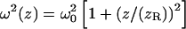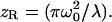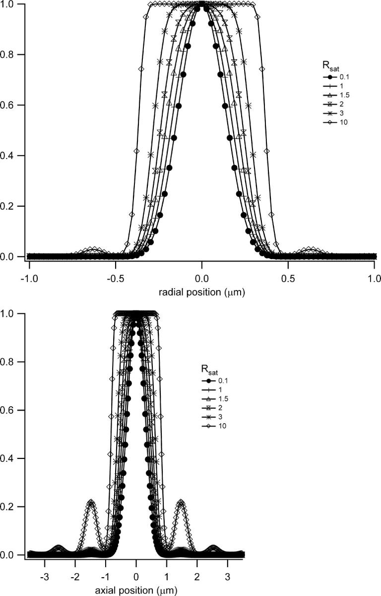
In cylindrical coordinates the GL distribution function is written as with and Raleigh range Here ω₀ defines the 1/e² laser beam radius at the focal plane and λ is the laser wavelength. The unsaturated volume for the GL distribution can be evaluated analytically and is found to be 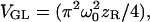with a γ-factor of γ_GL = 3/16. Using the GL model for the PSF, we can compute the effective molecular excitation profiles at various excitation rates with Eq. 7. The results are shown in Figs. 1 and 2, in which the effective molecular excitation profiles are shown for different excitation intensities relative to the saturation intensity. For notational convenience, we introduce the saturation parameter, which specifies the excitation intensity relative to the saturation intensity. It is important to recognize that the saturation intensity is dependent on the particular fluorescent species, and that R_sat thus depends not only on the photon flux of the excitation laser source but also on the absorption cross-section of the fluorescent entity being observed and therefore implicitly on the excitation wavelength as well. Moreover, in the laboratory one typically controls the average power on the sample rather than the intensity. Since power and intensity are related through the beam waist of the focused excitation and laser repetition rate, for a given excitation power the value of R_sat will also depend on the focused beam waist and repetition rate.

FIGURE 1.

Saturation-modified profiles of the fluorescence observation volume. Shown are radial (a) and axial (b) slices across the volume for different degrees of saturation. The enlarged and flatter profiles have important effects on the calibration of fluctuation spectroscopy measurements.

FIGURE 2.

Surface plots representing the observation volume in the absence (a) or presence (b) of excitation saturation.

Inspection of Figs. 1 and 2 demonstrates clearly the dramatic increase in the size of the excitation profile as the excitation intensity is increased, corresponding to a larger observation volume. The altered shape of the profile, with a flat region in the center, is also quite apparent. The size of the observation volume and corresponding γ-factors can be computed numerically using Eqs. 2 and 3, respectively. The absolute volume size, of course, depends upon the beam waist for the excitation PSF, but the scaling of the volume for different values of R_sat is independent of the beam waist. We thus compute a volume scaling factor by normalizing the computed volume at a given excitation level to the nonsaturated volume. The absolute volume for a particular experimental setup is calculated by multiplying the volume scaling factor, which fully accounts for saturation effects, by the nonsaturated GL volume, V_GL. The γ-factors computed at different R_sat values are also independent of the beam waist. The volume scaling factors and γ-factors are plotted in Figs. 3 and 4. Fig. 4 also shows the scaling of the ratio which we denote χ_γ/V, at different excitation levels. We note that at an excitation intensity corresponding to one-half of the saturation intensity the volume has already increased by ∼10%. At the saturation intensity (R_sat = 1) the volume has increased by 45% over the unsaturated volume, and by three times the saturation intensity the volume has increased by a factor of 6. In fact, the computed volume scaling factor for the GL excitation PSF can increase indefinitely, although at some point the fluorescence detection optics will limit the measured fluorescence signal and thus the volume as well. For comparison purposes, the volume scaling factors computed with the 3DG excitation PSF are also plotted in Fig. 3. As shown in the figure, the volume scaling factor for the 3DG model increase more slowly with increasing excitation power than the GL volume, reflecting the artificial and nonphysical limit of the 3DG excitation profile along the optical axis.

FIGURE 3.

The observation volume increases dramatically due to excitation saturation. This figure illustrates the volume scaling for the GL and 3DG profiles, which relate the volume for a particular excitation condition to the volume in the absence of saturation.

FIGURE 4.

The observation volume-profile changes alter the γ-factors, and the γ-factors are thus excitation-rate-dependent. The ratio of the γ-factors and observation volumes are also plotted here, and represent the expected amplitudes of measured correlation functions under different excitation conditions.

We next consider how the saturation-modified excitation profiles influence measured correlation curves. Once the excitation profiles are calculated, it is a relatively straightforward procedure to evaluate the correlation curves numerically using Fourier transforms to compute the required convolution integrals (28). To highlight the importance of volume and γ-factor shifts in FCS, we have computed the molecular excitation profiles and corresponding correlation curves for a series of excitation intensities. The computations assume a purely diffusive basis for the fluorescence fluctuations, concentration of 10 molecules/μm³, diffusion coefficient of 3 × 10⁻⁶ cm²/s, and beam waist of 0.4 μm, with 780-nm laser excitation. The resulting FCS curves are shown in Fig. 5. We note that the amplitude of the correlation functions is dramatically reduced by saturation, as is expected according to Eq. 6 due to the increasing observation volume. The correlation amplitude has decreased by 7% at one-half the saturation intensity, 23% at the saturation intensity, and has decreased by more than a factor of 2, at excitation powers corresponding to twice the saturation intensity. A corresponding increase in the apparent diffusion time also accompanies the increased volume size, as should also be expected for the larger volume profile. To highlight this relaxation time shift, the inset in Fig. 5 shows the same correlation curves normalized to unity. Higher excitation intensities correspond to the curves shifted toward the right. The apparent diffusion time has increased by a factor of 1.6 when the excitation intensity is twice the saturation intensity. We emphasize that these curves were all computed for a single fixed concentration, and the amplitude and timescale changes are due solely to variations in the γ-factor and the volume.

FIGURE 5.

Correlation curves were computed for a variety of excitation conditions under the influence of saturation. Saturation causes the amplitude of the correlation curves to decrease and the relaxation timescale to increase. The amplitude of the correlation curves decreases monotonically with the value R_sat. The inset shows the same curves normalized to unity to highlight the increasing relaxation times. Curves are shifted monotonically to the right with increasing saturation levels. Correlation curves were computed for a concentration of 10 molecules/μm³, diffusion coefficient of 3 × 10⁻⁶ cm²/s, and beam waist of 0.4 μm, with 780-nm laser excitation.

An interesting feature of the correlation curves displayed in Fig. 5 is that even though they are highly influenced by saturation, up until the highest values of R_sat any one of them can be fit quite well using the unsaturated 3DG-based FCS function in Eq. 5. However, such fits result in excitation-power-dependent changes in the calibration of the measurement system, suggesting that the beam waist of the excitation laser PSF and measured concentration are excitation-power-dependent—which, of course, they are not. Nonetheless, in practice one can calibrate the volume for a particular excitation condition, and subsequent FCS curves acquired under constant excitation conditions (i.e., with the same absorption cross-section and laser intensity) can be analyzed successfully using Eq. 5 without accounting explicitly for saturation-induced volume and profile changes. However, as soon as the excitation conditions are altered this is no longer the case, and the excitation rate-dependent calibration of the volume can lead to errors in data analysis. It is thus very useful to find a suitable method to apply the results introduced above for curve fitting in FCS. In principle, one can numerically calculate the FCS curves directly within the fitting routine using the same procedures used to compute the curves shown in Fig. 5. However, this approach is impractical since it is computationally intensive, and curve-fitting would be quite slow. Moreover, it is highly desirable to find relatively simple curve-fitting approaches such that they can be widely adopted.

We have therefore implemented a curve-fitting procedure that exploits the mathematical simplicity of the 3DG-based correlation function and makes use of the above noted condition that each of the individual computed FCS curves can be well fitted using the 3DG correlation function. The basic strategy is to apply the computed results from Fig. 5 to calibrate three R_sat-dependent scaling factors for the 3DG fitting functions. The amplitude scaling of the correlation functions is known precisely as a function of the relative excitation intensity, and is simply given by the scaling factor χ_γ/V introduced above and shown in Fig. 4. To determine the appropriate scaling for the effective relaxation times with saturation, the computed FCS curves of Fig. 5 were fit with the 3DG correlation function of Eq. 5. The fitting results provide a scaling law for the diffusion time, or equivalently of the effective beam waist, as a function of R_sat. Normalizing the effective beam waist to the beam waist of the corresponding PSF used to compute the correlation curves yields an intensity-dependent scaling factor, 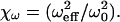We find a scaling factor for the axial beam waist along the optical axis, χ_z, in a similar manner. Both scaling factors are plotted in Fig. 6. It is reasonable that the effective beam waists scale differently with R_sat since the excitation PSF has unique profiles in the radial (Gaussian) and axial (Lorentzian) directions. The initial unsaturated value of the axial beam waist, z₀, was estimated in terms of the radial beam waist, ω₀, by curve-fitting the computed GL-based FCS curves with Eq. 5. We find their approximate relation to be 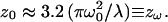Implementing this relationship in curve-fitting routines allows FCS analysis to be carried out using only a single free parameter for both the radial and axial beam waists.

FIGURE 6.

Scaling factors for the radial and axial beam waists, computed as described in the text.

Summarizing, Eq. 5 can be rewritten in the following form to be used for curve-fitting of FCS results when the excitation rates are varied:

(8)

Each of the scaling factors depends explicitly on R_sat, i.e., the excitation intensity relative to the saturation intensity, and I_sat becomes a new global fitting parameter in the data analysis. However, the scaling factors themselves are not fitting parameters—their values are uniquely determined by the value of the R_sat, which is known from the measurement power and the value of I_sat. The axial beam waist is also not a free parameter, but defined in terms of the radial beam waist and excitation wavelength as noted above. Therefore, this model specifies precisely how both the amplitude and diffusion times of the correlation curves should vary with R_sat, i.e., for different excitation powers or for molecules with different absorption cross-sections. Table 1 contains several values for these scaling factors for different values of R_sat. These values were programmed into a lookup table for use in curve-fitting. The scaling varies smoothly with R_sat, so additional values can be determined from this table by interpolation as necessary. It is important to note that the value of I_sat cannot be determined from a single FCS measurement. Instead, one must measure a series of FCS curves at different excitation levels and recover the saturation intensity parameter through global analysis of the entire data set. The free parameters for this global fit include the concentration, saturation intensity, and the beam waist (for instrument calibration with a known diffusion coefficient) or the diffusion coefficient (for known beam waist after initial calibration). Therefore, in principle, the fitting procedure outlined here can be used to analyze FCS data acquired over a wide range of excitation conditions (e.g., excitation power and absorption cross-sections) with only three free fitting parameters. Impressively, this is no more than is routinely used in standard FCS analysis that cannot account for saturation effects in the measurements. In practice, this analysis does, in fact, work quite nicely, although additional fitting parameters are typically required to account for the effects of photobleaching and/or triplet state dynamics, which are often also significant.

TABLE 1.

Effective scaling of the three-dimensional Gaussian parameters at different saturation levels

Rsat	0.1	0.2	0.3	0.5	0.7	1	1.5	2	3	4	5	6	8	10
χγ/V	1	0.99	0.97	0.93	0.87	0.76	0.59	0.45	0.28	0.19	0.14	0.11	0.07	0.05
χω	1	1.01	1.02	1.05	1.1	1.19	1.40	1.65	2.18	2.63	3.12	3.57	4.50	5.43
χz	1	1	1	1	1	1.04	1.21	1.44	2.3	4	6.2	10.2	25	41

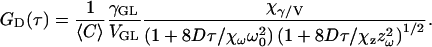
To demonstrate the performance of the method based on the saturation model, we performed a series of measurements for a Rhodamine 6G sample at different excitation levels (Fig. 7). Measurements were made at average excitation powers of 3, 4, 6, 8, 10, 12, 14, 16, 18, 20, 24, 28, 35, 40, and 50 mW, although several of these curves have been omitted from the graph for visual clarity. With increasing excitation power we observed both temporal and amplitude changes of the correlation curves as expected. However, both the amplitude and the relaxation time were decreasing with increasing power. The decreasing amplitude is caused by saturation, whereas the decreasing relaxation timescale indicates that photobleaching was also significant in these measurements. Photobleaching reduces the measured relaxation time, as molecules “disappear” from the measurement due to bleaching before they would otherwise have diffused out of the observation volume. Bleaching also tends to reduce the concentration of fluorescent molecules and thus increase the amplitude of the measured correlation curves, limiting the overall reduction in the amplitude due to saturation. To date, there has been no exact treatment of how photobleaching affects FCS measurements, but there is a commonly used approach that has proven to provide a reasonable description (29–32). In the presence of photobleaching, the diffusion-based correlation function of Eq. 8 is multiplied by the photobleaching factor 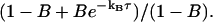Here k_B is the power-dependent average bleaching rate, and B is the average bleached fraction of the molecules in the observation volume.

FIGURE 7.

Fluorescence cross-correlation curves measured for Rhodamine 6G in water at different excitation levels. The curves were fit to the saturation model using a global fitting routine as described in the text. For visual clarity, not all measured excitation powers are shown.

The measured data series was thus fit with the bleaching-factor-modified Eq. 8, using a global fitting routine programmed in Igor Pro (Wavemetrics, Lake Oswego, OR). The diffusion coefficient was held fixed with the value 3 × 10⁻⁶ cm²/s. The concentration 〈C〉, beam waist ω₀ of the excitation PSF, and saturation intensity I_sat served as global free parameters. Each measurement power had unique bleaching factors. The excitation intensity for each measurement was used as a fixed parameter in the fitting routines to calculate R_sat as the saturation intensity parameter varied during fitting. Using this procedure, we find good quality fits for much of the measured data series as shown in Fig. 7. A subset of the individual curve-fitting results and associated residuals are plotted in Fig. 8. The corresponding behavior of the recovered bleaching parameters is shown in Fig. 9. We emphasize that these fits are achieved for the entire data set with only three global free parameters in addition to the bleaching parameters at each measurement power, and the model fits both the amplitude and the temporal relaxation of the measured correlation curves. The recovered beam waist and average excitation power corresponding to the saturation intensity were 0.38 μm and 7 mW, respectively. This means saturation effects become important in these measurements with as low as 2 or 3 mW average power at the sample. Based on rough estimates of the absorption cross-section and laser pulse width, one would expect the saturation intensity parameter of 10–15 mW, although the measured value is of the correct order of magnitude. Although it remains to be determined, we suspect the discrepancy is mainly due to the mismatch between the actual laser beam waist and the waist recovered from the 3DG-based fitting model, and that the actual beam waist may be somewhat smaller than the recovered fitting parameter value. The temporal profile of the laser pulses, which is not actually Gaussian as assumed, can also play a significant role in this discrepancy.

FIGURE 8.

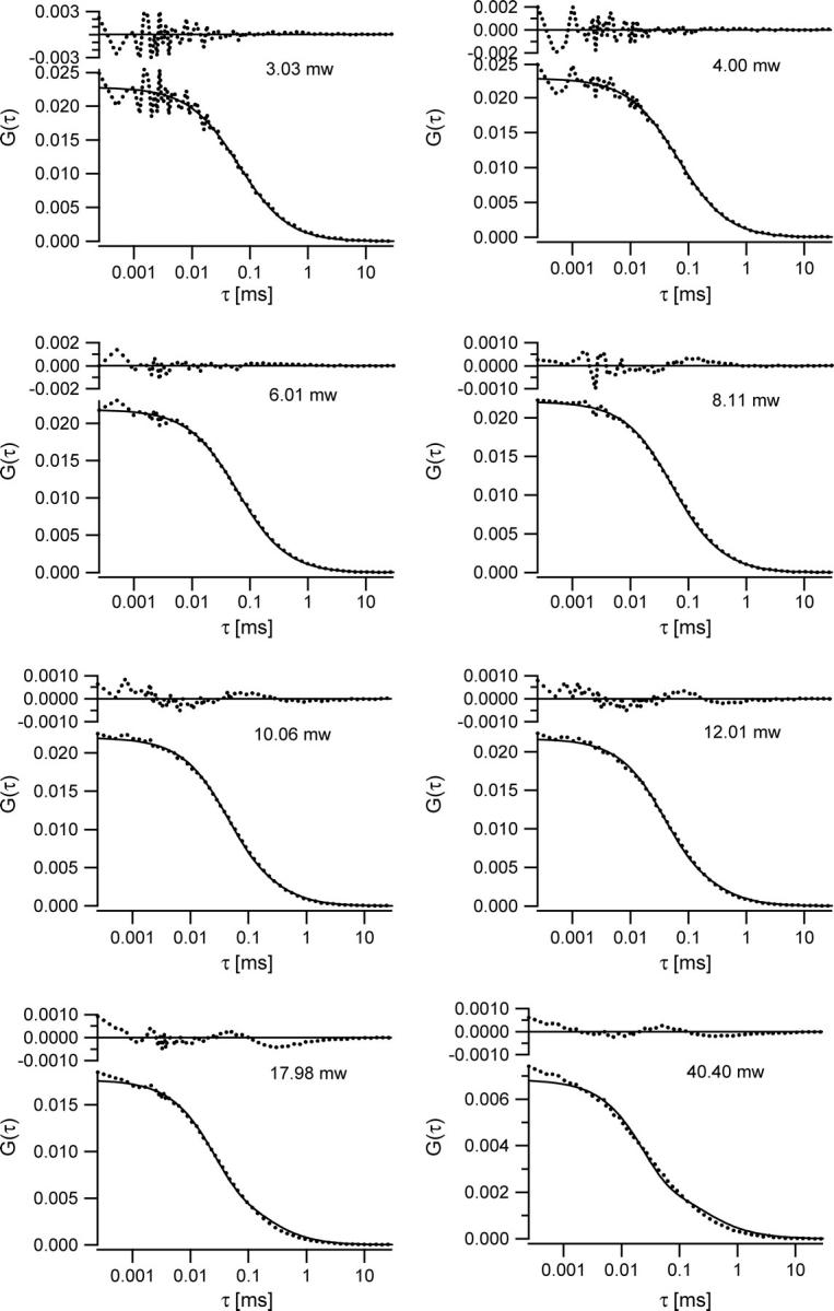
A selection of the fitted curves from Fig. 7 are shown here with residuals to highlight both the goodness of fit at lower excitation powers and the slight systematic deviations between the data and fits at higher excitation powers.

FIGURE 9.

The photobleaching rate (k_b) and bleached fraction (B) recovered from the global fitting analysis.

There is some systematic variation between the data and fits at the highest excitation powers, as shown in Fig. 8. Nonetheless, the model introduced here is quite successful at determining both the amplitude and approximate relaxation timescale of the measured correlation curves even at the highest excitation powers. The observed deviations may be due to several factors. First, for R_sat values >∼4, the 3DG-based FCS fitting functions begin to show some small systematic deviation from the exact FCS curve profiles shown in Fig. 5. Perhaps more importantly, the published models used to describe the photobleaching effects assume that the bleaching rate is constant across the observation volume, which clearly can lead to some systematic deviation. We expect that more accurate models for the bleaching process in FCS would help eliminate some of the observed deviations. An additional benefit of this work is that the quantitative treatment of saturation in FCS is likely to facilitate further systematic investigation of photobleaching effects in FCS measurements, which otherwise is not possible, since changing the excitation power changes the instrument calibration. Despite some minor systematic deviations in the fitted curves at the highest saturation levels, the good agreement between the measured data and the saturation theory fits with relatively few free fitting parameters gives good confidence in the accuracy of this treatment of the saturation effects.

Now that we have demonstrated that observation volume changes can clearly play an important role in FCS measurements, and a quantitative theory for modeling these effects, it remains to be discussed how important these observations are in a typical FCS experiment, and more importantly whether or not this quantitative description of the changes can be useful in FCS and other fluctuation spectroscopy applications. In some cases measurements can be performed at low excitation rates such that saturation does not play a significant role. In such circumstances there is clearly no need for a saturation modified theory. On the other hand, since saturation can become important with relatively low average excitation flux there may often be experiments where it is difficult to avoid saturation and still achieve good signal/noise ratios in fluctuation measurements. Even in such cases, however, the modified theory is not particularly essential, provided one makes all measurements with constant excitation power using only fluorescent molecules with relatively equivalent absorption cross-sections. On the other hand, if one wishes to make measurements using probes with largely differing absorption cross-sections or has a need to vary the excitation power, the new procedures introduced here will clearly be valuable. In fact, failure to account for saturation in such cases could lead to serious artifacts in FCS measurements. For example, with an instrument calibrated at a particular value for R_sat and a measurement performed at another (e.g., different power, different absorption cross-section) the recovered fitting parameters will not be correct. Depending on the degree to which R_sat changes between the calibration and real measurements, this could lead to misinterpretations of the data. For example, if one of the low power curves from Fig. 7 is used to calibrate our measurement, and a higher power curve is then fit using this calibration, it will not be possible to fit the data as the single component diffusion model. On the other hand the curve could be nicely fit with a two-component diffusion model, which clearly would be an incorrect interpretation of the data. The capability to avoid such potential artifacts, even when measuring FCS curves at different excitation intensities or for molecules with different cross-sections, is one clear reason why the quantitative treatment of saturation can be valuable. This capability can also be particularly valuable for multicolor applications of FCS, where absorption cross-sections for the multiple fluorophores used in a single measurement are likely to be different.

We believe this quantitative treatment of how fluctuation measurements scale with excitation power (or absorption cross-section) also has the potential to be of significantly broader use in FCS measurements. A problem facing analysis of FCS data in general is the selection of an appropriate physical model for curve-fitting. When appropriate models are selected, very accurate information can often be recovered through curve-fitting of the FCS data. On the other hand, the measured curves provide very limited clues to assist with model discrimination. The capability to use the procedures introduced here to analyze FCS data with quantitative accuracy with changing excitation conditions, e.g., average power at the sample, can provide an important tool for model verification in FCS analysis by testing whether recovered fitting parameters scale appropriately with power. For example, if bleaching or triplet-state models are included in a fitting analysis, as they often are by necessity, even at relatively low excitation powers, one would expect the bleaching or triplet-crossing rates would increase proportionally with excitation power. Diffusion coefficients or chemical kinetic rates, on the other hand, should not change with excitation rates. It has previously not been possible to perform such measurements to verify fitting models because changing the excitation power would change the instrument calibration in an unknown manner even at quite modest average excitation powers. With the tools introduced here this problem has been removed, and using this approach it will be possible to perform FCS measurements under varied excitation conditions. In some cases this may include measurements at high powers, but more importantly it may be used to acquire data at two different but still relatively low excitation powers. We believe this can become an important tool for verifying that the correct fitting functions are applied in FCS analysis. Finally, when the system under investigation is not harmed by high power excitation, it generally leads to higher signal/noise ratios in measured data. Thus, although some caution is certainly always warranted to avoid excessively high powers and the related complications that can arise from too much excitation power, using the ideas introduced here it should, in certain types of samples, be possible to work with relatively high excitation rates while maintaining the capability to interpret measured results in terms of physically relevant parameters.

CONCLUSIONS

Based on a fundamental physical model of the fluorescence excitation, we described the effects of excitation saturation on FCS measurements and provided a curve-fitting routine for analysis of correlation curves measured with varied fluorescence excitation conditions. The fitting function is based on the simple analytical form of the correlation function for the 3DG point spread function, and the amplitude and the shape of the correlation function is corrected by power and absorption cross-section-dependent scaling factors. We have shown that this procedure can successfully describe the amplitude and relaxation timescales for FCS curves measured over a wide range of excitation powers. This quantitative description of the variation in observed fluctuation data can be very useful in practical applications of fluctuation spectroscopy and may help users avoid measurement artifacts in calibrating FCS instrumentation. More importantly, as discussed above, we believe this treatment may lead to an important tool for model verification for data analysis in fluctuation spectroscopy.

APPENDIX

The Gaussian Lorentzian (GL) spatial profile for the point spread function (PSF) provides an accurate representation of the focused laser profile when the objective lens is underfilled with a Gaussian beam. We here explore whether the results computed using the GL profiles can be more generally applied to account for the volume scaling and correlation curve modifications that occur when using a more precise computation of the focused laser profile. We conclude that the saturation-induced volume and beam waist scaling laws introduced above can be successfully applied to analyze FCS data regardless of the degree to which the objective lens is over- or underfilled. We employ well-established procedures to precisely compute the excitation laser profile for a variety of laser illumination conditions (27,33). The degree of beam expansion before the objective lens is quantified in terms of the overfilling factor, which is defined as the ratio of the size of the back aperture of the objective lens to the size of the laser beam waist at the back aperture. We have computed the PSF profiles for several different overfilling factors, including 0.3, 0.5, 0.8, 1.2, 1.4, and 2.0, with smaller numbers corresponding to more overfilling. Using these profiles, it is a straightforward procedure to compute the saturation-modified profiles as described in Eq. 7. A representative set of such radial and axial profiles are shown in Fig. 10, which was computed for a filling factor of 0.3 (overfilled). We stress that the plotted profiles already account for the two-photon excitation process, which tends to suppress the relative amplitudes of the secondary peaks relative to the central peak. One can see that the radial profiles are mostly very similar to the GL profiles until the secondary peaks become apparent at very high excitation rates. The axial profiles are also rather similar to the GL profiles, although the difference becomes greater as saturation begins to modify the effective excitation profiles, and one can easily see the increasing amplitude of the secondary peaks relative to the main peak with increasing excitation powers. We then followed the procedures outlined above to compute the observation volumes, γ-factors, and FCS profiles for several different values of R_sat for each of the overfilling factors. The scaling of the volume looks visually the same as that shown in Fig. 3. The scaling of the γ-factor for different overfilling factors is shown in Fig. 11. One can clearly see the effects of the various focused laser profiles on the effective shape of the observation volume from the different scaling of the γ-factors with excitation rate. However, in computing the scaling at different excitation rates of χ_γ/V (the ratio of the γ-factor to the volume) for different overfilling factors, we find that χ_γ/V is independent of the degree to which the objective lens is overfilled. This result is shown in Fig. 12. Moreover, we find that the computed FCS autocorrelation curves associated with the excitation profiles for different overfilling factors and saturation levels can also be fit by a three-dimensional Gaussian-based fitting function, using the same scaling laws for the beam waists that we introduced for the GL profiles. We note that these fits are not perfect, and some systematic deviations can be seen in the fit residuals for most of the fitted curves when using the GL-based scaling laws, as shown in Fig. 13. However, the amplitude of the residuals relative to the correlation curve values is extremely small, as shown in the figure. Since the noise levels present in most real experimentally measured data sets are significantly larger than the amplitudes of these residuals relative to the correlation curve absolute values, we conclude one can safely employ the curve-fitting strategies introduced in this work without significant concern about the subtle differences between the GL model and the actual PSF. A broader interpretation of this finding is that, at least for two-photon excitation for which the secondary peaks of the volume are suppressed relative to the central peak, one need not, in general, be worried about subtle systematic problems from applying 3DG-based fitting models, regardless of the objective overfilling factor. The one exception to this conclusion is that for the higher values of R_sat (∼≥5) there are important differences between the two PSF distributions. The details of this exception will be reported in a forthcoming publication.

FIGURE 10.

Effective excitation profiles for varying degrees of excitation saturation computed for an objective lens overfilling factor of 0.3. The secondary peaks are more pronounced for the axial profiles than for the radial profiles.

FIGURE 11.

Scaling of the γ-factor at different excitation rates for several different values of the overfilling factor.

FIGURE 12.

The scaling of the γ-factor divided by the volume is independent of the overfilling factor. The amplitude scaling of correlation curves with varying saturation levels is therefore independent of the beam expansion before the objective lens.

FIGURE 13.

Fitting residuals for a series of FCS curves computed for several different filling factors and saturation levels. The fits were performed using the GL-based scaling for the amplitude and beam waists. Although there is some systematic deviation in these fits, it is quite small relative to the amplitudes of the fitted correlation curves, which had G(0) values ranging from 0.06 to 0.4. Any systematic deviation is, therefore, not of much practical importance, given the amplitude of typical noise levels in real measured data.

References

- 1.Rigler, R. , and E. S. Elson, editors. 2001. Fluorescence Correlation Spectroscopy Theory and Applications. Springer, New York. 486 p.
- 2.Chen, Y., J. D. Muller, P. T. C. So, and E. Gratton. 1999. The photon counting histogram in fluorescence fluctuation spectroscopy. Biophys. J. 77:553–567. [DOI] [PMC free article] [PubMed] [Google Scholar]
- 3.Kask, P., K. Palo, D. Ullmann, and K. Gall. 1999. Fluorescence-intensity distribution analysis and its application in biomolecular detection technology. Proc. Natl. Acad. Sci. USA. 96:13756–13761. [DOI] [PMC free article] [PubMed] [Google Scholar]
- 4.Hess, S. T., S. Huang, A. A. Heikal, and W. W. Webb. 2002. Biological and chemical applications of fluorescence correlation spectroscopy: a review. Biochemistry. 41:697–705. [DOI] [PubMed] [Google Scholar]
- 5.Schwille, P. 2001. Fluorescence correlation spectroscopy and its potential for intracellular applications. Cell Biochem. Biophys. 34:383–408. [DOI] [PubMed] [Google Scholar]
- 6.Chen, Y., J. D. Muller, Q. Ruan, and E. Gratton. 2002. Molecular brightness characterization of EGFP in vivo by fluorescence fluctuation spectroscopy. Biophys. J. 82:133–144. [DOI] [PMC free article] [PubMed] [Google Scholar]
- 7.Chen, Y., L.-N. Wei, and J. D. Mueller. 2003. Probing protein oligomerization in living cells with fluorescence fluctuation spectroscopy. Proc. Natl. Acad. Sci. USA. 100:15492–15497. [DOI] [PMC free article] [PubMed] [Google Scholar]
- 8.Thompson, N. L., A. M. Lieto, and N. W. Allen. 2002. Recent advances in fluorescence correlation spectroscopy. Curr. Opin. Struct. Biol. 12:634–641. [DOI] [PubMed] [Google Scholar]
- 9.Bacia, K., and P. Schwille. 2003. A dynamic view of cellular processes by in vivo fluorescence auto- and cross-correlation spectroscopy. Methods. 29:74–85. [DOI] [PubMed] [Google Scholar]
- 10.Magde, D., E. Elson, and W. W. Webb. 1972. Thermodynamic fluctuations in a reacting system. Measurement by fluorescence correlation spectroscopy. Phys. Rev. Lett. 29:705–708. [Google Scholar]
- 11.Qian, H., and E. L. Elson. 1990. Analysis of confocal laser-microscope optics for 3-D fluorescence correlation spectroscopy. Appl. Opt. 30:1185–1195. [DOI] [PubMed] [Google Scholar]
- 12.Schwille, P., U. Haupts, S. Maiti, and W. W. Webb. 1999. Molecular dynamics in living cells observed by fluorescence correlation spectroscopy with one- and two-photon excitation. Biophys. J. 77:2251–2265. [DOI] [PMC free article] [PubMed] [Google Scholar]
- 13.Berland, K. M., P. T. C. So, and E. Gratton. 1995. Two-photon fluorescence correlation spectroscopy: method and application to the intracellular environment. Biophys. J. 68:694–701. [DOI] [PMC free article] [PubMed] [Google Scholar]
- 14.Cianci, G. C., J. Wu, and K. M. Berland. 2004. Saturation modified point spread functions in two-photon microscopy. Microsc. Res. Tech. 64:135–141. [DOI] [PubMed] [Google Scholar]
- 15.Berland, K. M., and G. Shen. 2003. Excitation saturation in two-photon fluorescence correlation spectroscopy. Appl. Opt. 42:5566–5576. [DOI] [PubMed] [Google Scholar]
- 16.Mertz, J. 1998. Molecular photodynamics involved in multi-photon excitation microscopy. Eur. Phys. J. D. 3:53–66. [Google Scholar]
- 17.Denk, W., J. H. Strickler, and W. W. Webb. 1990. Two-photon laser scanning fluorescence microscopy. Science. 248:73–76. [DOI] [PubMed] [Google Scholar]
- 18.Xu, C., and W. W. Webb. 1997. Multiphoton excitation of molecular fluorophores and nonlinear laser microscopy. In Topics in Fluorescence Spectroscopy. J. Lakowicz, editor. Plenum Press, New York. 471–540.
- 19.Elson, E. L., and D. Magde. 1974. Fluorescence correlation spectroscopy. I. Conceptual basis and theory. Biopolymers. 13:1–27. [DOI] [PubMed] [Google Scholar]
- 20.Thompson, N. L. 1991. Fluorescence correlation spectroscopy. In Topics in Fluorescence Spectroscopy. J.R. Lakowicz, editor. Plenum Press, New York. 337–378.
- 21.Mertz, J., C. Xu, and W. W. Webb. 1995. Single-molecule detection by two-photon-excited fluorescence. Opt. Lett. 20:2532–2534. [DOI] [PubMed] [Google Scholar]
- 22.Webb, W. W. 2001. Fluorescence correlation spectroscopy: inception, biophysical experimentations, and prospectus. Appl. Opt. 40:3969–3983. [DOI] [PubMed] [Google Scholar]
- 23.Koppel, D. E. 1974. Statistical accuracy in fluorescence correlation spectroscopy. Phys. Rev. A. 10:1938–1945. [Google Scholar]
- 24.Rigler, R., U. Mets, J. Widengren, and P. Kask. 1993. Fluorescence correlation spectroscopy with high count rate and low background: analysis of translational diffusion. Eur. Biophys. J. 22:169–175. [Google Scholar]
- 25.Siegman, A. 1986. Lasers. University Science Books, Mill Valley, CA.
- 26.Wohland, T., R. Rigler, and H. Vogel. 2001. The standard deviation in fluorescence correlation spectroscopy. Biophys. J. 80:2987–2999. [DOI] [PMC free article] [PubMed] [Google Scholar]
- 27.Richards, B., and E. Wolf. 1959. Electromagnetic diffraction in optical systems. II. Structure of the image field in an aplanatic system. Proc. R. Soc. Lond. A. 253:358–379. [Google Scholar]
- 28.Hess, S. T., and W. W. Webb. 2003. Focal volume optics and experimental artifacts in confocal fluorescence correlation spectroscopy. Biophys. J. 83:2300–2317. [DOI] [PMC free article] [PubMed] [Google Scholar]
- 29.Widengren, J., R. Rigler, U. Mets, and K. I. S. S. Dep. 1994. Triplet-state monitoring by fluorescence correlation spectroscopy. J. Fluoresc. Med. Biochem. Biophys. 4:255–258. [DOI] [PubMed] [Google Scholar]
- 30.Widengren, J., U. Mets, and R. Rigler. 1995. Fluorescence correlation spectroscopy of triplet states in solution: a theoretical and experimental study. J. Phys. Chem. 99:13368–13379. [Google Scholar]
- 31.Widengren, J., and R. Rigler. 1996. Mechanisms of photobleaching investigated by fluorescence correlation spectroscopy. Bioimaging. 4:149–157. [Google Scholar]
- 32.Dittrich, P. S., and P. Schwille. 2001. Photobleaching and stabilization of fluorophores used for single-molecule analysis with one- and two-photon excitation. Appl. Phys. B. 73:829–873. [Google Scholar]
- 33.Stamnes, J. J., and V. Dhayalan. 1996. Focusing of electric-dipole waves. Pure Appl. Opt. 5:195–225. [Google Scholar]