Dipolar Coupling between Nitroxide Spin Labels: The Development and Application of a Tether-in-a-Cone Model

Abstract

A tether-in-a-cone model is developed for the simulation of electron paramagnetic resonance spectra of dipolar coupled nitroxide spin labels attached to tethers statically disordered within cones of variable halfwidth. In this model, the nitroxides adopt a range of interprobe distances and orientations. The aim is to develop tools for determining both the distance distribution and the relative orientation of the labels from experimental spectra. Simulations demonstrate the sensitivity of electron paramagnetic resonance spectra to the orientation of the cones as a function of cone halfwidth and other parameters. For small cone halfwidths (<∼40°), simulated spectra are strongly dependent on the relative orientation of the cones. For larger cone halfwidths, spectra become independent of cone orientation. Tether-in-a-cone model simulations are analyzed using a convolution approach based on Fourier transforms. Spectra obtained by the Fourier convolution method more closely fit the tether-in-a-cone simulations as the halfwidth of the cone increases. The Fourier convolution method gives a reasonable estimate of the correct average distance, though the distance distribution obtained can be significantly distorted. Finally, the tether-in-a-cone model is successfully used to analyze experimental spectra from T4 lysozyme. These results demonstrate the utility of the model and highlight directions for further development.

INTRODUCTION

Site-directed spin-labeling (SDSL) methods are being widely used to study both the structure and the functional dynamics of proteins (for reviews, see Hubbell and Altenbach and others (1–6)). SDSL combines site-directed mutagenesis to introduce single cysteines at specific sites within a protein together with labeling by a cysteine-specific nitroxide probe, typically methanethiosulfonate spin label (MTSSL). Electron paramagnetic resonance (EPR) spectroscopy is then used to measure physical characteristics at that site including the mobility of the spin label and the accessibility of the side chain to relaxation agents such as O₂ and Ni(EDDA). In double site-directed spin-labeling (DSDSL) studies, pairs of nitroxide spin-label probes are introduced at selected sites. EPR spectroscopy is then used to measure the distance or distance distribution between probes (for recent examples, see Klare et al. and others (7–14)). Distances obtained from DSDSL studies have been used to build models of protein structures and the structural transitions associated with protein function (e.g., 10,15,16). Reviews of various techniques for using EPR to measure interprobe distances have been recently collected in a single volume (17).

Continuous wave EPR (CW-EPR) spectroscopy can be used to measure distances up to 20–25 Å, whereas pulsed EPR methods can be used to measure distances up to 80 Å in favorable cases (18). Distances and distance distributions can be extracted from CW-EPR spectra of dipolar coupled nitroxides by a variety of approaches. In the case where the two nitroxides adopt a unique geometry with respect to each other, a single interelectron distance has been determined by computer lineshape simulation (19). In other cases, the use of different sets of assumptions allows distance determination by analysis of line height ratios (20), by measurement of the homogeneous linewidth (21), or by Fourier deconvolution/convolution methods (22–25). Various methods for measuring distances in the 7–24-Å range have been compared experimentally (26).

When two nitroxides adopt a specific, rigid geometry with respect to each other, both the relative distance and orientation between the two nitroxides can be determined by computer lineshape simulation (for reviews, see Hustedt and Beth (4,27)). In a study using a spin-labeled NAD⁺ ligand bound to polycrystalline glyceraldehyde-3-phosphate dehydrogenase (GAPDH), CW-EPR spectra were obtained at X-, Q-, and W-bands. Starting from the spin Hamiltonian and using a combination of simulated annealing and Marquardt-Levenberg algorithms, these multifrequency spectra were simultaneously analyzed by direct spectral simulation to obtain the distance between the unpaired electrons localized to the N-O bond of the nitroxides, the orientation of the interelectron vector in the frame of the nitroxide A- and g-tensors, and the three angles defining the relative orientation of the two nitroxide tensor frames (19).

Fourier methods assume the lineshape to be the convolution of a dipolar broadening function with the sum of the spectra of the isolated probes at the two sites (22–25). These methods inherently assume that there is an isotropic averaging of the relative orientation between the nitroxides and are used to obtain estimates of the average interspin distance and the width of the distance distribution.

Fourier convolution methods and the spectral simulation approach used to analyze data for spin-labeled NAD⁺ bound to GAPDH represent two extremes. Fourier convolution methods have been successfully used to give interspin distances in a number of studies. On the other hand, the highly ordered nature of the spin-labeled NAD⁺/GAPDH complex required the detailed consideration of the orientation of the nitroxides. These results raise questions about the analysis of data from DSDSL studies where there is often partial ordering between the two probes. The apparent mobility of the MTSSL side chain depends strongly on the label site (28). Labels at buried sites give EPR spectra indicative of immobilized labels, as can labels at sites that have some degree of tertiary contact. Steric interactions at these sites restrict the local dynamics of the MTSSL side chain. The mobility of the MTSSL side chain, as reflected in the inverse of the central linewidth, is a measure of both the amplitude and the rate of constrained anisotropic rotational diffusion (5). Simulations of the X-band EPR lineshapes from MTSSL and other methanethiosulfonate spin labels at helix surface sites in T4 lysozyme (T4L) have been used to determine rates and the associated order parameters of rotational dynamics (29). Similar results have been obtained from a combined analysis of spectra collected at 9 and 250 GHz (30). These results indicate that the local motion of the MTSSL side chain is highly constrained, the overall motion of the probe is coupled to the backbone, and the lineshape of MTSSL retains sensitivity to backbone dynamics even at helix surface sites (5). Similarly it is important to consider whether because of the site-specific constraints on the local order of the MTSSL side chains, the EPR spectrum of a pair of dipolar coupled labels retains sensitivity to their relative orientation. Careful consideration of the effects of the relative orientation of the probes may lead to increased accuracy in the determination of the relative distance distribution between probes. In addition, the relative orientation may itself be used as a constraint for building structural models.

The vast majority of SDSL studies of protein structure utilize the MTSSL label, which has five chemical bonds between the α-carbon of the cysteine and the five-membered nitroxide ring. Although detailed consideration of the preferred orientation and flexibility about each of these bonds is possible (29,31), in this work a simple model is developed in an initial attempt to treat the inherent flexibility of the tether linking the nitroxide to the protein in the context of simulation of the EPR spectra of dipolar coupled spin labels. The unpaired electron is placed at the end of a tether that adopts all possible angles within a cone of variable halfwidth. Hence, both the interelectron distance and the relative orientation of the two nitroxides are determined by the position of the tethers within their cones. This model then, inherently, produces a distribution of interelectron distances. At the same time, the degree of orientational disorder between the probes is also a function of the various parameters of the model. The tether-in-a-cone model can thus be used to test the sensitivity of CW-EPR spectra of dipolar coupled nitroxides to the degree of disorder in both the interelectron distance and orientation.

Simulations are presented below that demonstrate the sensitivity of EPR spectra to the various parameters of the tether-in-a-cone model. In particular, these simulations demonstrate the sensitivity of CW-EPR spectra to the relative orientation of the two cones as a function of the cone halfwidth. These simulations are used to determine how much disorder is required to obscure the effects of the relative orientation of the spin labels. These simulations are then used as artificial data for analysis by a Fourier convolution method. The distance distributions obtained by Fourier convolution analysis are compared to the known distance distributions from the tether-in-a-cone model. From these results, it can be determined how well the Fourier convolution method does as a function of the degree of disorder. Finally, the tether-in-a-cone model can itself be used as a tool for analyzing data from DSDSL studies as demonstrated by analysis of selected data from DSDSL studies of T4L.

Portions of this work have been previously published as an abstract (32).

METHODS

Tether-in-a-cone model

The spin Hamiltonian in the high-field approximation for a pair of dipolar coupled nitroxides is given by

(1)

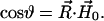
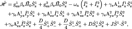
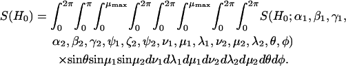
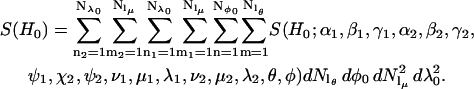
where β_e is the Bohr magneton, g¹ and g² are the tensors defining the interaction of the electron spin of nitroxide 1 () and nitroxide 2 () with the DC magnetic field (), ω_n is the Larmor frequency of the nitrogen nucleus, γ_e is the gyromagnetic ratio for the electron, A¹ and A² are the hyperfine tensors defining the interaction of the nitrogen nuclear spins ( or ) with or D is the unique element of the dipolar coupling tensor, and J is the scalar exchange interaction. Treatment of this spin Hamiltonian has been described in detail (4,19). The g-tensor and the hyperfine (A-) tensor elements for the two nitroxides, as well as the dipolar coupling tensor, D, are all determined by a set of Euler angle transformations (see Fig. 1). In the tether-in-a-cone model, the nitroxides are placed at the end of tethers of length, q, which are separated by a distance, p, at their bases. The tethers adopt all possible angles within cones of halfwidth μ_max resulting in a distribution of internitroxide distances and orientations.

FIGURE 1.

Diagram defining parameters for the tether-in-a-cone model. The axes X, Y, and Z are the axes of the two nitroxides with X along the N-O bond and Z perpendicular to the plane of the nitroxide and with all subscripts referring to nitroxide 1 or nitroxide 2. The two cones are separated by at their bases and their relative orientation is determined by the angles ψ₁, ζ₂, and ψ₂ (ζ₂ not shown). The orientation of the two cones with respect to the magnetic field, is determined by the angles θ and φ (φ not shown). The orientations of the tethers, and within their respective cones are determined by the angles ν, μ, and λ (ν and λ not shown). The orientation of the tethers with respect to the nitroxide axis systems are determined by the angles α, β, and γ (α and γ not shown). Those angles that are not shown for the sake of simplicity correspond to Euler angle rotations about the appropriate Z axis as defined in Eqs. 2–8.

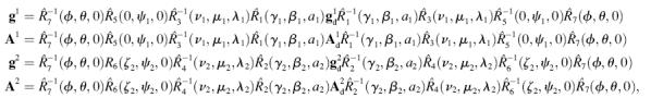
A set of seven rotation operators define the various transformations that are needed to determine the elements of the nitroxide g- and A-tensors and the dipolar coupling tensor. The orientations of the tether axes with respect to the two nitroxide axis frames are determined by the transformations and for nitroxides 1 and 2, respectively. The orientations of the tether axes within the cones are determined by the transformations and 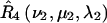for nitroxides 1 and 2, respectively. The orientation of the two cones with respect to each other is determined by for nitroxide 1 and for nitroxide 2. Finally, the orientation of the nitroxide pair with respect to the magnetic field is determined by the transformation, Using this set of Euler angle transformations, the g- and A-tensor elements in the laboratory frame for nitroxides 1 and 2 are given by

(2)

where and are the diagonal g-tensors and and are the diagonal A-tensors for the two nitroxides. All of the Euler angle rotation matrices are defined as follows,

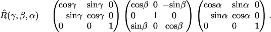(3)

In this work it is assumed that the two nitroxides have the same principal values for their g- and A-tensors (g_xx = 2.0082, g_yy = 2.0060, g_zz = 2.0023, A_xx = 6.5 Gauss, A_yy = 5.5 Gauss, A_zz = 36.0 Gauss) except as noted below for the analyses of data from T4L.

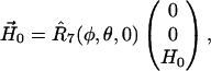
The dipolar coupling depends on the angle, between the interelectron vector, and the magnetic field vector,

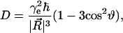(4)

where

(5)

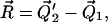
The vector is determined by

(6)

and written as

(7)

with

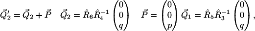(8)

where and are vectors representing the two tethers and is the vector of length p connecting their respective origins (see Fig. 1).

A spectrum is calculated by averaging over a set of angles to account for an isotropic distribution of nitroxide pairs in the lab frame (as determined by θ and φ) and to account for a range of tether positions within the two cones assuming square-well potentials of equal halfwidth (μ_max).

(9)

For a pair of ¹⁴N nitroxide spin labels, there are nine possible combinations of nitrogen nuclear spin states. For each nuclear spin state there are four allowed electron spin transitions. Therefore, S(H₀;α₁,β₁,γ₁,α₂,β₂,γ₂,ψ₁,ζ₂,ψ₂,ν₁,μ₁,λ₁,ν₂,μ₂,λ₂,θ,φ) is the sum of 36 first-derivative Lorentzian lineshapes. The calculation of the center position and transition probabilities from the spin Hamiltonian (Eq. 1) for each of these Lorentzian lines has been described in detail elsewhere (19). In all of the calculations presented here a Lorentzian linewidth of 2.0 Gauss is used except as noted below for the analyses of data from T4L.

A number of different spherical codes for efficient averaging over the surface of a sphere as required by Eq. 9 have been used for simulation of EPR spectra (33–35). In this work a variation of the SPIRAL code (36,37) has been used. The SPIRAL code defined below is equivalent to that previously used by Wong and Roos (37) in defining a set of θ values but differs slightly in how the corresponding values of φ are generated. Let

(10)

then

(11)

and

(12)

The value of N_loop determines the tightness of the spiral, i.e., the number of turns from φ = 0 to 2π as θ goes from π (or π/2) to 0. A total of spirals are used with each spiral starting at equally spaced values of φ from 0 to 2π.

Equations 10–12 define a SPIRAL code for averaging over the angles θ and φ. The SPIRAL code for averaging over the cone angles μ and λ is defined using a similar set of equations with μ restricted between 0 ≤ μ ≤ μ_max. A third angle, ν, which corresponds to rotation about the tether axis, is also included. Note that rotations by the angle ν do not change the interelectron distance.

(13)

In all of the simulations presented in this work, it is assumed that the lengths of the tethers q = |Q₁|= |Q₂| and the angles defining the orientations of the tethers with respect to the nitroxide, γ = γ₁= γ₂ and β = β₁ = β₂, are the same for both labels. For all the calculations presented here, N_ν = 1 and ν is fixed to be 0°. Using the SPIRAL codes as defined in Eqs. 10–13, the integral in Eq. 9 becomes

(14)

In the tether-in-a-cone model, the interelectron distance, R, is a function of the values of p and q, the relative orientation of the two cones (as determined by the angles ψ₁, ζ₂, and ψ₂), and the cone angles μ and λ for both nitroxides. Averaging over the angles μ₁, λ₁, μ₂, and λ₂ results in a distribution of interelectron distances, P(R). The values of R obtained by averaging over these angles are binned and P(R) is represented as a histogram at 99 values of R between R = 0 and R = p + 3q. The distance distribution, P(R), is characterized by its average value, 〈R〉,

(15)

and its standard deviation, σ_R,

(16)

Convolution analysis

Convolution-based methods have been widely used to analyze EPR spectra of dipolar coupled nitroxides (22–25). It is assumed that the spectrum of the dipolar coupled nitroxides, C(H₀), is given by the convolution of the spectrum of the spatially isolated nitroxides, M(H₀), with a dipolar broadening function, Δ(H₀).

(17)

The function Δ(H₀) is assumed to be a sum of Pake patterns corresponding to a distribution of interspin distances. Rabenstein and Shin (23) obtained Δ(H₀) by Fourier deconvolution of experimentally determined C(H₀) and M(H₀) spectra and then determined an average distance and width of the distance distribution from Δ(H₀). Noise in the Fourier transform of Δ(H₀), which is an inherent result of deconvolution, can be dealt with by fitting to a sum of two Gaussian functions (25,38). Alternatively, Steinhoff and co-workers (24) avoided the deconvolution step by assuming a Gaussian distribution of interspin distances to calculate Δ(H₀), convolving Δ(H₀) and M(H₀), comparing the result to the experimental data, and finding the Gaussian distance distribution that gave the best fit. Hubbell and co-workers (22) have developed an interactive approach using a combination of deconvolution and convolution steps to obtain a histogram of interspin distances.

In this work, the approach of Steinhoff and co-workers is used (24). The distribution of interspin distances, P_G(R), is taken to be a Gaussian centered at R₀ of width κ_R.

(18)

The broadening function, Δ(H₀), is calculated as the sum of a large number (100,000 or more) of Pake patterns. A lower limit distance cutoff, determined by the sweep width (SW, in Gauss) of the experimental spectra, R_min(Å) = 30.3 × SW^(−1/3), is used so as not to include Pake patterns whose singularities lie outside of the scan range of the data being analyzed. A dipolar broadened spectrum is calculated by convolving Δ(H₀) and M(H₀). The fit between the calculated spectrum and the spectrum being analyzed is then optimized by adjusting R₀ and κ_R using Marquardt-Levenberg methods to minimize χ², the sum of the squares of the differences between the data and the fit (see Hustedt et al. (39)). In some cases, the distance distribution, P_G(R), was taken to be the sum of two Gaussians. The fitting parameters are then the centers and widths of the two Gaussians and their relative amplitudes. When analyzing simulated spectra of dipolar coupled nitroxides, the spectrum of the spatially isolated nitroxides, M(H₀), was calculated by setting p = 100 Å, q = 0 Å, and μ_max = 0°. When analyzing data from DSDSL studies of T4L, M(H₀) was taken to be the equally weighted sum of the normalized EPR spectra of the two spin-labeled single cysteine mutants at the corresponding sites.

The quality of the fits to the data is expressed by the correlation coefficient

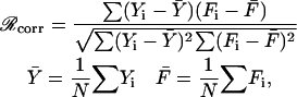(19)

where Y_i are the values of the data, F_i are the values of the fit to the data, and N is the total number of points in each. To account for incomplete labeling when analyzing data from DSDSL experiments on T4L, the best fit to the data was obtained as a linear combination of: 1), the spectrum of the spatially isolated nitroxides, M(H₀), 2), the calculated spectrum of dipolar coupled nitroxides, C(H₀), and 3), a constant baseline correction as described previously (19).

(20)

Analysis of data using the tether-in-a-cone model

The tether-in-a-cone model has been incorporated into a computer software package designed for the nonlinear least-squares analysis of EPR spectra (19,39). The program uses a combination of simulated annealing and Marquardt-Levenberg algorithms to find the best fit parameters to a given spectrum. The principal values of the g-tensors, and and A-tensors, and were obtained from fitting the EPR spectra of the corresponding spin-labeled single cysteine mutants as previously described (39). The Lorentzian linewidth was taken to be the average value obtained from the analysis of the two singly labeled spectra. Values of β, γ, and q were obtained from the X₄X₅ model (29) as described below. Values of p have been estimated from the C_α to C_α distance measured from the crystal structure of wild-type T4L (Protein Data Bank (PDB), 3LZM (40)). Data from DSDSL studies of T4L were analyzed using a combination of multiple independent runs of simulated annealing followed by further minimization by the Marquardt-Levenberg algorithm and rigorous determination of confidence intervals (19,39) in an attempt to find the values of ψ₁, ζ₂, ψ₂, and μ_max, which give the global χ² minimum. To account for incomplete labeling, the best fit to the data was obtained as a linear combination of: 1), the equally weighted sum of the spectra of the spin-labeled single cysteine mustants, M(H₀), 2), the calculated spectrum of dipolar coupled nitroxides, S(H₀), and 3), a constant baseline correction as described previously (19).

(21)

Computer software

All computer programs used to generate the tether-in-a-cone-model simulations and to perform the analyses of data were written in FORTRAN. Anyone interested in obtaining the FORTRAN code developed in this work should contact the authors.

X₄X₅ model

The X₄X₅ model proposed by Hubbell and co-workers (29,31) has been used to obtain estimated values for the two angles that determine the orientation of the tether axis with respect to the nitroxide frame, γ and β, and the tether length, q. In the X₄X₅ model the torsion angles of the first three bonds between the C_α of the labeled cysteine and the nitroxide ring are fixed, whereas the torsion angles for the fourth and fifth bonds are allowed to adopt all possible angles between 0 and 360°. From the x-ray crystal structure of spin-labeled mutants of T4L, the MTSSL at a solvent-exposed site is expected to have X₁ ≈ −60°, X₂ ≈ −60°, and X₃ ≈ −90° or X₃ ≈ +90° (29,31). Using the known structure of T4L (PDB, 3LZM (40)), the appropriate residue was mutated to cysteine and labeled with MTSSL in the conformation X₁ = −60°, X₂ = −60°, and X₃ = −90°. The torsion angles were set using the University of California San Francisco Chimera package (Computer Graphics Laboratory, UCSF; supported by National Institutes of Health (NIH) P41 RR-01081). Using the PyMOL molecular graphics system (Delano Scientific LLC, San Carlos, CA), the nitroxide ring was rotated in steps of 30° about X₄ and X₅ and the appropriate coordinates saved at each step. From the set of 144 orientations, average values of various parameters relating the nitroxide to the C_α of the labeled cysteine residue were calculated. For a spin label at residue 65 of T4L, the values calculated are 〈q〉 = 7.08 Å, 〈β〉 = 78.9°, and 〈γ〉 = 330.5°. Very similar results have been obtained for spin labels at the other T4L sites (61, 68, and 69) that have been labeled in this study and using an alternate conformation (X₁ = 180°, X₂ = +60°, and X₃ = +90°).

SDSL of T4 lysozyme

Plasmids containing the cysteine-less T4L gene and certain mutants (single cysteine mutants at sites 65 and 69, double cysteine mutants at 65/68 and 65/69) were generously provided by Dr. Hassane Mchaourab (Vanderbilt University, Nashville, TN). Other cysteine mutations (single cysteine mutants at sites 61 and 68, double cysteine mutant at 61/65) were engineered into the cysteine-less T4L gene by the overlap extension method (41). For all the T4L mutants, the entire coding region was confirmed by DNA sequencing. T4L mutants were expressed and purified as previously described (28). Briefly, plasmids were transformed into competent Escherichia coli K38 cells; 1 mM isopropyl β-thiogalactoside was added to log phase cultures to induce protein expression for 90 min. The cell pellet was resuspended in a buffer containing 25 mM Tris, 25 mM MOPS, and 0.2 mM EDTA (pH 7.6). The cells were then disrupted by sonication. After 30 min centrifugation at 10,000 rpm, the supernatant was passed through a 0.22-μm filter. The flowthrough was then loaded on a Resource S cation-exchange column (Amersham Bioscience, Piscataway, NJ) and eluted with a NaCl gradient from 0 to 1 M. Protein concentration was determined by ultraviolet absorption at 280 nm using an extinction coefficient of 1.228 cm²mg⁻¹. The purity of all T4L mutant proteins was at least 95%, as determined by SDS-PAGE (42). Single or double cysteine mutants were spin labeled with a 10-fold or 20-fold molar excess of 1-oxyl-2,2,5,5-tetramethyl-Δ3-pyrroline-3-methyl methanethiosulfonate spin label (Toronto Research Chemicals, North York, Ontario, Canada) at room temperature for 10 min and then at 4°C overnight. Unreacted label was removed from all samples using a HiTrap desalting column (Amersham Bioscience, Piscataway, NJ) with desalting buffer containing 100 mM NaCl, 20 mM MOPS, 0.1 mM EDTA, and 0.02% azide (pH 7.0). Proteins were then concentrated in an Amicon Ultra-4 centrifugal filter device (5 kDa nominal molecular weight limit; Millipore, Bedford, MA).

EPR spectroscopy

All EPR spectra were collected at X-band using a Bruker EMX spectrometer (BrukerBiospin, Billerica, MA) equipped with a TM₁₁₀ cavity with a Dewar insert and a Bruker variable temperature control unit. All spectra were recorded at −30°C using 100 kHz Zeeman modulation of 1 Gauss amplitude and a microwave power of 5 mW. Samples of spin-labeled T4L in desalting buffer plus 70% (w/w) glycerol were placed in 50-μl glass capillaries (VWR International, West Chester, PA) and flame sealed. The 50-μl capillaries were placed in a 5-mm quartz tube containing silicone fluid (Thomas Scientific, Swedesboro, NJ) held within the Dewar insert.

RESULTS

Model calculations

Fig. 2 shows simulations calculated for the tether-in-a-cone model as a function of the distance between the bases of the two cones, p, with all other parameters fixed. For comparison, the upper simulation (Fig. 2 A) is a spectrum of spatially isolated nitroxides where p = 100 Å, q = 0 Å, and μ_max = 0° so that 〈R〉 = 100 Å, σ_R = 0 Å, and the dipolar coupling is effectively zero. The other panels show simulations for p = 16 Å (Fig. 2 B), p = 12 Å (Fig. 2 C), and p = 8 Å (Fig. 2 D) with q = 6 Å and μ_max = 30°. The insets at the upper right of these panels (and in subsequent figures) show histograms representing the interspin distance distribution, P(R). As p decreases, the center of P(R) moves to shorter distances and the corresponding simulated EPR spectrum becomes broader, which is indicative of increased dipolar coupling.

FIGURE 2.

EPR spectra calculated for the tether-in-a-cone model as a function of p. α = β = γ = 0°, ψ₁ = 90°, ζ₂ = 0°, and ψ₂ = 90°. (A) p = 100 Å, q = 0 Å, and μ_max = 0°. For all other calculations q = 6 Å; μ_max = 30°; and (B) p = 16 Å, (C) p = 12 Å, (D) p = 8 Å. For panels B–D, the insets (top right) show a histogram representing the distance distribution, P(R).

Fig. 3 shows the effect of increasing the tether length, q, with all other parameters fixed. As the tether length is increased from q = 2 Å (Fig. 3 A) through q = 6 Å (Fig. 3 B) to q = 10 Å (Fig. 3 C), splittings that are clearly resolved at the high and low field z-turning points in the simulated spectra for the smallest tether lengths are broadened out as the width of the distance distribution, P(R), increases accordingly. Fig. 4 shows similar results as a function of the cone halfwidth for μ_max = 10° (Fig. 4 A), μ_max = 30° (Fig. 4 B), and μ_max = 60° (Fig. 4 C). As the cone halfwidth increases, resolved dipolar splittings in the spectra are broadened out and the width of P(R) increases. The calculations shown in Figs. 3 B and 4 B have been performed for the same values of q = 6 Å and μ_max = 30°. Given the orientation of the cones as determined by the angles ψ₁ = 90°, ζ₂ = 0°, and ψ₂ = 90°, this results in a distance distribution centered at 〈R〉 = 12.05 Å with a width of σ_R = 1.88 Å. Reducing the tether length to q = 2 Å (Fig. 3 A; 〈R〉 = 12.02 Å and σ_R = 0.71 Å) or reducing the cone halfwidth to μ_max = 10° (Fig. 4 A; 〈R〉 = 12.00 Å and σ_R = 0.62 Å) have similar effects on the resulting distance distribution and EPR spectra. Increasing the tether length to q = 10 Å (Fig. 3 C; 〈R〉 = 12.56 Å and σ_R = 3.49 Å) or increasing the cone halfwidth to μ_max = 60° (Fig. 4 C; 〈R〉 = 12.05 Å and σ_R = 3.34 Å) likewise have similar effects on the resulting distance distribution and EPR spectra.

FIGURE 3.

EPR spectra calculated for the tether-in-a-cone model as a function of q. α = β = γ = 0°; ψ₁ = 90°; ζ₂ = 0°; ψ₂ = 90°; p = 12 Å; μ_max = 30°; and (A) q = 2 Å, (B) q = 6 Å, (C) q = 10 Å. The insets (top right) show a histogram representing P(R).

FIGURE 4.

EPR spectra calculated for the tether-in-a-cone model as a function of μ_max. α = β = γ = 0°; ψ₁ = 90°; ζ₂ = 0°; ψ₂ = 90°; p = 12 Å; q = 6 Å; and (A) μ_max = 10°, (B) μ_max = 30°, (C) μ_max = 60°. The insets (top right) show a histogram representing P(R).

Fig. 5 shows simulations for the tether-in-a-cone model calculated for various values of four angles (β, ψ₁, ζ₂, ψ₂) for fixed values of p = 8 Å, q = 6 Å, and μ_max = 30°. Comparing the spectra in Fig. 5, A (β = 0°) and B (β = 90°), shows that the simulated EPR spectra depend strongly on the orientation of the tether axis in the frame of the nitroxide, whereas the corresponding distance distributions are independent of the angles α, β, and γ (results for α and γ not shown). The spectra in Fig. 5, A and C–F, show the effect of changes in the relative orientation of the two cones as determined by the angles ψ₁, ζ₂, and ψ₂. The relative orientation of the cones is represented by the diagrams at the left of each panel in Fig. 5 and in subsequent figures. Both the average and the width of the distance distribution depend strongly on the relative orientation of the cones. Therefore, the lineshape changes observed in Fig. 5 as a function of ψ₁, ζ₂, and ψ₂ do not reflect changes in cone orientation alone but also reflect significant changes in P(R). Fig. 6 shows the corresponding simulations for a larger value of the distance between the bases of the two cones (p = 12 Å, q = 6 Å, and μ_max = 30°). As in Fig. 5, the results of Fig. 6 show that the angles ψ₁, ζ₂, and ψ₂ influence both the EPR lineshape and the distance distribution, P(R).

FIGURE 5.

EPR spectra calculated for the tether-in-a-cone model as a function of various angles. For all calculations, p = 8 Å, q = 6 Å, and μ_max = 30°. (A) α = β = γ = 0° and ψ₁ = ζ₂ = ψ₂ = 0°. (B) α = 0°, β = 90°, γ = 0°, and ψ₁ = ζ₂ = ψ₂ = 0°. (C) α = β = γ = 0°, ψ₁ = 0°, ζ₂ = 0°, and ψ₂ = 90°. (D) α = β = γ = 0°, ψ₁ = 90°, ζ₂ = 0°, and ψ₂ = 90°. (E) α = β = γ = 0°, ψ₁ = 90°, ζ₂ = 90°, and ψ₂ = 90°. (F) α = β = γ = 0°, ψ₁ = 90°, ζ₂ = 180°, and ψ₂ = 90°. The insets (top right) show a histogram representing P(R). The diagrams to the left of each panel represent the relative orientation of the cones as determined by ψ₁, ζ₂, and ψ₂.

FIGURE 6.

EPR spectra calculated for the tether-in-a-cone model as a function of various angles. For all calculations, p = 12 Å, q = 6 Å, and μ_max = 30°. (A) α = β = γ = 0° and ψ₁ = ζ₂ = ψ₂ = 0°. (B) α = 0°, β = 90°, γ = 0°, and ψ₁ = ζ₂ = ψ₂ = 0°. (C) α = β = γ = 0°, ψ₁ = 0°, ζ₂ = 0°, and ψ₂ = 90°. (D) α = β = γ = 0°, ψ₁ = 90°, ζ₂ = 0°, and ψ₂ = 90°. (E) α = β = γ = 0°, ψ₁ = 90°, ζ₂ = 90°, and ψ₂ = 90°. (F) α = β = γ = 0°, ψ₁ = 90°, ζ₂ = 180°, and ψ₂ = 90°. The insets (top right) show a histogram representing P(R). The diagrams to the left of each panel represent the relative orientation of the cones as determined by ψ₁, ζ₂, and ψ₂.

The results in Figs. 5 and 6 demonstrate that the average value and width of P(R) are determined, in part, by the angles ψ₁, ζ₂, and ψ₂. Both 〈R〉 and σ_R are also determined by p, q, and μ_max. To isolate the effects of the cone orientation on the calculated EPR spectrum, the five simulations shown in Fig. 7 have been performed for different values of ψ₁, ζ₂, and ψ₂ with p, q, and μ_max adjusted so that P(R) is approximately equal for the different cone orientations. Using the distance distribution calculated for ψ₁ = 0°, ζ₂ = 0°, and ψ₂ = 90°, p = 10.66 Å (adjusted so that 〈R〉 = 8 Å), q = 6 Å, and μ_max = 30° as a template, values of p, q, and μ_max were obtained by nonlinear least-squares analysis, which best fit this P(R) for alternate values of ψ₁, ζ₂, and ψ₂. From the parameter sets obtained in this way, the EPR spectra and P(R) distributions in Fig. 7 were then calculated. As shown in Table 1, the parameters used in Fig. 7 all give a P(R) with 〈R〉 ≈ 8 Å and σ_R ≈ 1.5 Å. The calculations in Figs. 8–10 have been performed in a similar way so that within each figure, all simulations give distance distributions that have approximately the same values of 〈R〉 and σ_R. The results in Fig. 8 were calculated starting with ψ₁ = ζ₂ = ψ₂ = 90°, p = 8.51 Å, q = 6 Å, and μ_max = 10° giving a P(R) with 〈R〉 ≈ 12 Å and σ_R ≈ 0.7 Å. Likewise for Fig. 9, all of the calculations gave a distance distribution with 〈R〉 ≈ 12 Å and σ_R ≈ 1.9 Å; and for Fig. 10, 〈R〉 ≈ 12 Å and σ_R ≈ 3.4 Å. It is apparent from these results that for small values of σ_R, there are large differences in the calculated EPR spectrum as a function of ψ₁, ζ₂, and ψ₂ (see Fig. 8). These differences are reduced at intermediate values of σ_R (see Fig. 9) and are small or negligible at larger values of σ_R (see Fig. 10). Each one of the simulations in Figs. 7–10 (solid gray lines) was then analyzed using a Fourier convolution method and the results are overlaid (dashed black lines) as described below.

FIGURE 7.

EPR spectra (solid gray lines) calculated for the tether-in-a-cone model to show the effect of cone orientation for 〈R〉 ≈ 8 Å and σ_R ≈ 1.5 Å. The values of p, q, μ_max, ψ₁, ζ₂, and ψ₂ are given in Table 1. For all calculations, α = β = γ = 0°. The fits obtained by the Fourier convolution method are shown as dashed black lines. The diagrams to the left of each panel represent the relative orientation of the cones as determined by ψ₁, ζ₂, and ψ₂. The insets to the right show the actual distance distribution (gray histogram) for the simulated EPR spectrum and the distance distribution (black line) obtained by the Fourier convolution method.

TABLE 1.

Parameters for Figs. 7–10

Figure	p (Å)	q (Å)	μmax	ψ1	ζ2	ψ2	〈R〉 (Å)*	σR (Å)†	R0 (Å)‡	κR (Å)‡	ℛcorr§
7 A	7.13	2.96	102.29°	0°	0°	0°	7.97	1.48	7.78	1.40	0.987
7 B	10.66	6	30°	0°	0°	90°	8.00	1.51	7.35	2.00	0.985
7 C	7.91	9.00	13.75°	90°	0°	90°	8.06	1.50	7.72	0.93	0.959
7 D	5.46	4.27	35.20°	90°	90°	90°	8.01	1.51	7.89	1.82	0.972
7 E	6.50	2.80	58.05°	90°	180°	90°	8.06	1.46	7.83	1.57	0.991
8 A	11.80	2.23	69.97°	0°	0°	0°	12.01	0.63	12.71	1.09	0.971
8 B	16.89	8.78	8.16°	0°	0°	90°	12.00	0.62	12.13	0.47	0.919
8 C	11.99	6.05	8.34°	90°	0°	90°	12.00	0.62	14.01	1.59	0.889
8 D	8.51	6	10°	90°	90°	90°	12.00	0.64	12.49	0.71	0.913
8 E	7.69	4.67	17.09°	90°	180°	90°	12.01	0.63	12.43	0.55	0.938
9 A	11.03	4.25	91.00°	0°	0°	0°	12.07	1.83	12.77	2.72	0.992
9 B	16.15	7.48	29.24°	0°	0°	90°	11.96	1.86	12.62	1.87	0.977
9 C	11.90	5.20	30.52°	90°	0°	90°	12.05	1.88	13.49	2.69	0.965
9 D	8.69	6	30°	90°	90°	90°	12.00	1.87	12.78	1.82	0.965
9 E	10.39	3.51	54.77°	90°	180°	90°	12.01	1.86	12.84	2.25	0.990
10 A	9.80	5.68	119.23°	0°	0°	0°	12.07	3.27	12.78	4.35	0.989
10 B	13.77	10.26	42.53°	0°	0°	90°	11.97	3.38	12.85	4.26	0.992
10 C	11.49	6.11	50.11°	90°	0°	90°	12.05	3.34	13.29	4.01	0.989
10 D	9.12	6	60°	90°	90°	90°	11.99	3.39	12.61	4.32	0.991
10 E	10.20	4.60	92.04°	90°	180°	90°	12.03	3.39	12.26	4.82	0.992

^*From Eq. 15.

^†From Eq. 16.

^‡From Eq. 18.

^§From Eq. 19.

FIGURE 8.

EPR spectra (solid gray lines) calculated for the tether-in-a-cone model to show the effect of cone orientation for 〈R〉 ≈ 12 Å and σ_R ≈ 0.6 Å. The values of p, q, μ_max, ψ₁, ζ₂, and ψ₂ are given in Table 1. For all calculations, α = β = γ = 0°. The fits obtained by the Fourier convolution method are shown as dashed black lines. The diagrams to the left of each panel represent the relative orientation of the cones as determined by ψ₁, ζ₂, and ψ₂. The insets to the right show the actual distance distribution (gray histogram) for the simulated EPR spectrum and the distance distribution (black line) obtained by the Fourier convolution method.

FIGURE 9.

EPR spectra (solid gray lines) calculated for the tether-in-a-cone model to show the effect of cone orientation for 〈R〉 ≈ 12 Å and σ_R ≈ 1.9 Å. The values of p, q, μ_max, ψ₁, ζ₂, and ψ₂ are given in Table 1. For all calculations, α = β = γ = 0°. The fits obtained by the Fourier convolution method are shown as dashed black lines. The diagrams to the left of each panel represent the relative orientation of the cones as determined by ψ₁, ζ₂, and ψ₂. The insets to the right show the actual distance distribution (gray histogram) for the simulated EPR spectrum and the distance distribution (black line) obtained by the Fourier convolution method.

FIGURE 10.

EPR spectra (solid gray lines) calculated for the tether-in-a-cone model to show the effect of cone orientation for 〈R〉 ≈ 12 Å and σ_R ≈ 3.4 Å. The values of p, q, μ_max, ψ₁, ζ₂, and ψ₂ are given in Table 1. For all calculations, α = β = γ = 0°. The fits obtained by the Fourier convolution method are shown as dashed black lines. The diagrams to the left of each panel represent the relative orientation of the cones as determined by ψ₁, ζ₂, and ψ₂. The insets to the right show the actual distance distribution (gray histogram) for the simulated EPR spectrum and the distance distribution (black line) obtained by the Fourier convolution method.

Convolution analysis

When using convolution-based methods to analyze the spectrum of a pair of dipolar coupled nitroxides, the assumption is made that the orientation effects that are explicitly modeled in the tether-in-a-cone model can be neglected. The results presented in Figs. 7–10 represent an opportunity to test the robustness of the convolution approach under situations resulting in a wide range of EPR lineshapes for dipolar coupled nitroxides.

The spectra simulated for the tether-in-a-cone model shown in Figs. 7–10 have been fit using a convolution approach (Eq. 17). The spectrum of the spatially isolated nitroxide, M(H₀), is shown in Fig. 2 A. The overlaid fits, C(H₀), are shown as dashed black lines in Figs. 7–10. The Gaussian distance distributions, P_G(R), are shown as black lines overlaid on the histogram of distances obtained from the tether-in-a-cone model. The results of analysis by the Fourier convolution method are summarized in Table 1, which gives the values of p, q, and μ_max along with the angles ψ₁, ζ₂, and ψ₂ used in the simulations. These six parameters determine the distance distribution, P(R), from the tether-in-a-cone model. The distance distribution is described by an average distance, 〈R〉, and variance, σ_R. The average distance, R₀, and width, κ_R, obtained by convolution analysis assuming a Gaussian distance distribution are also given in Table 1 as are the correlation coefficients (Eq. 19) for the fits obtained by the Fourier convolution method to the spectra simulated for the tether-in-a-cone model. The values of the correlation coefficients for the fits using the single Gaussian distance distributions are plotted in Fig. 11 versus q, μ_max, and σ_R. There is no apparent relation between the correlation coefficient and the tether length, q (Fig. 11 A). On the other hand, the correlation coefficient steadily increases with μ_max up to ∼40° (Fig. 11 B).

FIGURE 11.

Values of ℛ_corr for the fits to the tether-in-a-cone model simulations using the Fourier convolution method assuming a single Gaussian distance distribution (Figs. 7–10) are plotted versus q (A), μ_max (B), and σ_R (C).

The tether-in-a-cone model simulations in Figs. 7–10 have also been analyzed by the Fourier convolution method assuming a bimodal Gaussian distribution of distances. This approach does, in general, lead to modest improvements in the fit of the convolved spectrum to the tether-in-a-cone model simulation. Nevertheless, in all of the examples considered here, the correlation coefficient between the distance distribution, P(R), from the tether-in-a-cone model and the distance distribution, P_G(R), from the Fourier convolution method decreases when a bimodal Gaussian distance distribution is used. Fig. 12 A shows an example of a tether-in-a-cone model simulation fit by the Fourier convolution method assuming a bimodal Gaussian distance distribution. The fit obtained by the Fourier convolution method to the tether-in-a-cone model simulation is improved even as the use of a bimodal P_G(R) results in a less accurate representation of the true P(R) (cf. Fig. 7 B). As the correlation coefficient, ℛ_corr, for the EPR spectra increases from 0.985 to 0.993 on going from a single Gaussian to a bimodal Gaussian P_G(R), the correlation coefficient between P(R) and P_G(R) decreases from 0.936 to 0.848.

FIGURE 12.

Simulated EPR spectra (gray lines) analyzed using a Fourier convolution method assuming a bimodal Gaussian distribution. The fits obtained by the Fourier convolution method are shown as dashed lines. The insets show the actual distance distribution for the simulated EPR spectrum (gray histogram) and the distance distribution obtained by the Fourier convolution method (dashed line). (A) Same simulation as in Fig. 7 B. (B) Simulation is the sum of those in Figs. 7 B and 9 B. (C) Simulation is the sum of those in Figs. 7 B and 10 B. In the insets to panels B and C the dotted lines were obtained by fitting the histograms to a bimodal Gaussian distribution. The dotted spectra were generated by the Fourier convolution method using these bimodal Gaussian distributions.

Simulated EPR spectra that correspond to a truly bimodal distance distribution have also been analyzed by the Fourier convolution method assuming a bimodal Gaussian distribution of distances. The simulated spectrum (solid gray line) in Fig. 12 B is the equally weighted sum of those in Fig. 7 B (〈R〉 = 8 Å) and Fig. 9 B (〈R〉 = 12 Å). The simulated spectrum in Fig. 12 C is the equally weighted sum of those in Fig. 7 B (〈R〉 = 8 Å) and Fig. 10 B (〈R〉 = 12 Å). The best fits obtained by the Fourier convolution method assuming a bimodal Gaussian distribution of distances are shown as dashed lines. In both cases, the Fourier convolution method gives a good estimate (10.2 Å, Fig. 12 B; and 10.0 Å, Fig. 12 C) of the actual average distance between the labels (〈R〉 = 10.0 Å). Nevertheless, as shown in the insets at the top right of each panel, the bimodal P_G(R) recovered from Fourier convolution analysis (dashed lines) does not represent the true bimodal shape of the distance distribution (gray histogram). The dotted lines overlaid on the histograms in Fig. 12, B and C, were obtained by fitting the P(R) directly to a bimodal Gaussian distribution. The bimodal P_G(R) distributions so obtained were then used to generate the dotted lines overlaid on the spectra in Fig. 12, B and C. The spectral fits obtained by first fitting the distance distributions (dotted lines; ℛ_corr = 0.972 for Fig. 12 B and ℛ_corr = 0.982 for Fig. 12 C) are statistically worse than those obtained by fitting the spectra themselves (dashed lines; ℛ_corr = 0.989 for Fig. 12 B and ℛ_corr = 0.994 for Fig. 12 C).

Analysis of data

The EPR spectra of four spin-labeled single cysteine T4L mutants (61, 65, 68, and 69) and three spin-labeled double cysteine T4L mutants (61/65, 65/68, and 65/69) were collected at −30°C in 70% glycerol. Under these conditions the effect of the global tumbling of the protein and all local dynamics on the linear CW-EPR spectra are negligible and the spectra of the four single cysteine mutants are nearly identical. The four spectra of the singly labeled mutants were analyzed to give g- and A-tensor values and Lorentzian linewidths (results not shown). The three sum of singles EPR spectra (61 + 65, 65 + 68, and 65 + 69), given by the equally weighted sum of the normalized EPR spectra of the spin-labeled single cysteine mutants, are shown on the left side of Fig. 13 (green lines) with the EPR spectra of the three spin-labeled double cysteine mutants (61/65, 65/68, and 65/69) overlaid on an expanded scale (×5; black lines). The EPR spectra of the doubly labeled mutants are also shown on the right side of Fig. 13 (black circles) with the results of analysis by the convolution method (red lines) and the results of fitting to the tether-in-a-cone model (blue lines) overlaid.

FIGURE 13.

EPR spectra of spin-labeled T4 lysozyme mutants. Shown on the left are the sum of singles spectra (T4L 61 + T4L 65, T4L 65 + T4L 68, T4L 65 + T4L 69; green lines) with the spectra of the double cysteine mutants (T4L 61/65, T4L 65/68, T4L 65/69; black lines) overlaid on an expanded (×5) scale. The spectra of the double cysteine mutants are also shown on the right (black circles) with fits obtained to the tether-in-a-cone model (blue lines) and obtained by the convolution method (red lines) overlaid. The distance distributions obtained using both methods are plotted in the insets at the top right. All spectra were obtained as described in the text with the spin-labeled T4L mutants in desalting buffer plus 70% (w/w) glycerol at −30°C. Analysis of the spectra of the four single cysteine mutants gave the following parameters (fits not shown): T4L 61, g_xx = 2.00814, g_yy = 2.00606, g_zz = 2.00230, A_xx = 6.34 Gauss, A_yy = 5.45 Gauss, A_zz = 36.29 Gauss, Lorentzian linewidth Γ = 2.28 Gauss; T4L 65, g_xx = 2.00821, g_yy = 2.00603, g_zz = 2.00226, A_xx = 6.43 Gauss, A_yy = 5.54 Gauss, A_zz = 36.07 Gauss, Γ = 2.31 Gauss; T4L 68, g_xx = 2.00817, g_yy = 2.00606, g_zz = 2.00228, A_xx = 6.51 Gauss, A_yy = 5.27 Gauss, A_zz = 36.05 Gauss, Γ = 2.31 Gauss; T4L 69, g_xx = 2.00815, g_yy = 2.00602, g_zz = 2.00233, A_xx = 6.48 Gauss, A_yy = 5.35 Gauss, A_zz = 36.01 Gauss, Γ = 2.30 Gauss. The parameters obtained by fitting the three spectra of the double cysteine mutants to the tether-in-a-cone model are given in Table 2. Fits were obtained with the following parameters fixed: q = 7.08 Å, β = 78.9°, and γ = 330.5°. Values of p were fixed as given in Table 2. The parameters obtained by fitting the spectra of the double cysteine mutants using the convolution method were: T4L 61/65, R₀ = 7.51 Å and σ_R = 0.61 Å; T4L 65/68, R₀ = 10.61 Å and σ_R = 5.07 Å; T4L 65/69, Amplitude₁ = 1.00, (R₀)₁ = 7.51 Å, (σ_R)₁ = 0.61 Å, Amplitude₂ = 0.82, (R₀)₂ = 9.90 Å, and (σ_R)₂ = 5.57 Å. The inset at the center of the figure is a ribbon diagram representing the structure of T4L (PDB, 3LZM (40)) with the α-carbons of residues 61 (red), 65 (green), 68 (blue), and 69 (yellow) shown as colored spheres.

Using the Fourier convolution method, all three doubly labeled T4L spectra were fit assuming both a single and bimodal Gaussian distance distribution. The fits to the spectra for T4L 61/65 and T4L 65/68 were not significantly improved by the inclusion of a second Gaussian component, nor did the second component appreciably alter the average distance between the spin labels (results not shown). On the other hand, the fit to the spectra for T4L 65/69 was significantly improved by the inclusion of a second Gaussian component (fit assuming bimodal distribution is shown). The distributions from these fits are shown as insets on the right-hand side of Fig. 13 (red lines).

The parameters obtained from the fits to these three spectra using the tether-in-a cone model are given in Table 2. Multiple simulated annealing runs were performed to explore the full parameter space. For example, to fit the spectrum of T4L 61/65, 36 simulated annealing runs were performed, which gave values of ψ1, ζ₂, and ψ2 ranging from 0 to 180° (ψ1 and ψ2) or 0–360° (ζ₂) and the values of μ_max ranging from 2.8 to 57°. The parameters obtained from the simulated annealing runs that gave the better fits to the data as judged by χ² values all clustered near the best-fit values given in Table 2. These results, together with the confidence intervals discussed below, increased the likelihood that best-fit parameters obtained represent the true global χ² minimum. For these three spectra, the best-fit cone halfwidths range from 9 to 175° and the widths of the resulting distance distribution range from 0.8 to 3.9. The resulting distance distributions are shown as insets on the right-hand side of Fig. 13 (blue).

TABLE 2.

Parameters for Fig. 13

	ψ1*	ζ2*	ψ2*	μmax*	p (Å)†	Singly labeled‡	〈R〉 (Å)§	σR (Å)¶
61/65	98°	17°	89°	8.6°	6.18	7%	7.65	0.75
65/68	161°	171°	175°	175°	5.16	<1%	10.59	3.89
65/69	37°	139°	73°	73°	6.42	8%	8.30	2.83

^*Best fit values to data.

^†Measured C_α-C_α distance from crystal structure.

^‡Best fit percentage of the doubly integrated signal intensity from singly spin-labeled protein.

^§From Eq. 15.

^¶From Eq. 16.

The confidence intervals for the angle ζ₂ for the fits to the T4L data using the tether-in-a-cone model are shown in Fig. 14. The confidence intervals have been calculated by holding one parameter fixed to a series of values while varying other parameters to minimize χ² (43,44). In the case of T4L 61/65 (squares), ζ₂ is well determined with two local minima at ζ₂ ≈ 18° and ζ₂ ≈ 351°. In the case of T4L 65/68 (circles), ζ₂ is poorly determined. T4L 65/69 (triangles) represents an intermediate case with ζ₂ determined to be within a broad minimum centered at ζ₂ = 150°. Similar results were obtained for the angles ψ₁ and ψ₂ (not shown). These results show that the ability to resolve the relative orientation of the probes depends on the μ_max obtained from fitting the data.

FIGURE 14.

Confidence intervals for ζ₂ from the analysis of the spectra of the three spin-labeled double cysteine mutants of T4L using the tether-in-a-cone model. The values of χ² were obtained by adjusting ψ₁, ψ₂, and μ_max to obtain the best fit to the data at fixed values of ζ₂. The top panel shows the results plotted fullscale. The bottom panel shows an expanded scale. In both panels, each curve is scaled to its 99% confidence level calculated using the F-statistic (dashed line). Results are shown for T4L 61/65 (▪), T4L 65/68 (•), and T4L 65/69 (▴).

DISCUSSION

Tether-in-a-cone model simulations

Simulations showing the dependence of spectra for the tether-in-a-cone model on various parameters are presented in Figs. 2–6. These parameters include the distance, p, between the origins of the two tethers (Fig. 2), the tether length, q (Fig. 3), the halfwidth of the cone, μ_max (Fig. 4), the angle β that defines the orientation of the tether axis in the nitroxide frame (Figs. 5 and 6, A and B), and the orientation of the two cones with respect to each other as determined by the angles ψ₁, ζ₂, and ψ₂ (Figs. 5 and 6, A and C–F). In addition to the calculated EPR spectra, the corresponding distance distribution determined by the parameters of the tether-in-a-cone model are also shown. These distance distributions depend in the expected ways on these parameters. As p decreases, the average distance between the labels decreases (Fig. 2). As q (Fig. 3) and μ_max (Fig. 4) increase, the width of the distance distribution increases. Changes in the relative orientation of the cones change both the average and width of the distance distribution. For example, going from ψ₁ = ζ₂ = ψ₂ = 0° (Figs. 5 and 6 A) to ψ₁ = ζ₂ = 0° and ψ₂ = 90° (Figs. 5 and 6 C) both decreases 〈R〉 and significantly increases σ_R. In all of these calculations, the resulting EPR spectrum is consistent with the calculated distance distribution. The overall width of the spectrum increases as the strength of the dipolar coupling increases with decreasing 〈R〉 (e.g., Fig. 2). Resolved splittings due to dipolar coupling are lost as σ_R increases (e.g., Figs. 3 and 4).

The simulations in Figs. 5 and 6 present a broad range of lineshapes of dipolar coupled nitroxides that correspond well with the range of lineshapes reported in the literature (e.g., Altenbach et al. (22)). The average distance obtained in these spectral simulations range from 〈R〉 = 6.65 Å (Fig. 5 C) to 〈R〉 = 16.62 Å (Fig. 6 F) and the widths of the distance distributions range from σ_R = 0.46 Å (Fig. 6 A) to σ_R = 2.13 Å (Fig. 6 D). These results indicate that the tether-in-a-cone model can be used as a model for the analysis of data from DSDSL studies to determine the distance distribution between labels.

Effect of cone orientation

The tether-in-a-cone model has been developed, in part, to determine whether the relative orientation between spin labels can be measured in typical DSDSL experiments. This information has the potential to provide additional constraints for building structural models of proteins and protein complexes. In the tether-in-a-cone model, there are three angles that determine the relative orientation of the cones. When all other parameters are held constant, changes in cone orientation also produce changes in the distance distribution, P(R). To be able to separate the effects on EPR spectra of changes in cone orientation from changes in the P(R), simulations were performed with different cone orientations that result in approximately the same P(R). The simulations shown in Fig. 7 (〈R〉 ≈ 8 Å and σ_R ≈ 1.5 Å), Fig. 8 (〈R〉 ≈ 12 Å and σ_R ≈ 0.6 Å), and Fig. 9 (〈R〉 ≈ 12 Å and σ_R ≈ 1.9 Å) all show dependence on the relative orientation of the cones as determined by ψ₁, ζ₂, and ψ₂. The largest changes in the simulations are seen for the smallest values of σ_R as in Fig. 8. For the largest σ_R, as in Fig. 10 (〈R〉 ≈ 12 Å and σ_R ≈ 3.4 Å), the simulations are essentially independent of cone orientation.

The results in Figs. 7–10 suggest that under appropriate conditions it would be possible to determine the relative orientation of the spin labels and that the appropriate condition may be σ_R < 2 Å. However, there are reasons to believe that orientation effects are more closely related to the value of μ_max. First, for μ_max = 180°, the dependence on cone orientation will necessarily vanish independent of q and the resulting value of σ_R. Second, σ_R depends strongly on μ_max and q. The tether length for MTSSL in the X₄X₅ model ranges from 4.4 to 8.8 Å with an average value of 7.1 Å. For a tether length on the order of 7 Å, the simulations in Figs. 7–10 are also consistent with a condition that to observe orientation effects μ_max must be small. A close examination of these results suggests that 40° is a reasonable estimate for the upper limit on μ_max beyond which simulated spectra become largely independent of cone orientation. This value of 40° for the cone halfwidth corresponds to an order parameter of S = 0.68. As noted below, this estimate is consistent with the results obtained using the Fourier convolution method.

Analysis by convolution method

The simulations in Figs. 7–10 have been analyzed by a Fourier convolution method as though they were experimental data. An examination of these results suggests that the quality of the fit obtained by the convolution method depends on the width of the distance distribution, σ_R. Nevertheless, a plot of the quality of the fit as measured by ℛ_corr versus σ_R (see Fig. 11 C) shows that for small values of σ_R the quality of the fit can vary greatly. In fact, ℛ_corr is very closely correlated with the cone halfwidth, μ_max (Fig. 11 B). In contrast, ℛ_corr does not appear to be correlated with the tether length, q (Fig. 11 A). For example, of all the results in Fig. 8, the best correlation between the tether-in-a-cone model simulation and the Fourier convolution analysis is obtained for Fig. 8 A, which has the largest cone halfwidth, μ_max = 70°. The Fourier convolution method assumes isotropic averaging of the relative orientation of the probes, which corresponds to μ_max = 180°. Given that ℛ_corr depends strongly on μ_max as μ_max increases up to ∼40°, it can be inferred that μ_max = 40° is an approximate cutoff beyond which simulations for the tether-in-a-cone model become independent of cone orientation.

These results allow an evaluation of the ability of the Fourier convolution method to fit simulated data with a known distribution of internitroxide distances and a restricted distribution of relative orientations. Here the assumption is made that the dipolar coupled spectrum is given by the convolution of the spectrum of spatially isolated nitroxides with a broadening function given by a sum of Pake patterns corresponding to a Gaussian distribution of distances. The ability of the Fourier convolution method to recover the true distance distribution can be determined by examining the insets in Figs. 7–10. Although in most of the cases considered (17 out of 20) the value of R₀ obtained is within 1 Å of the actual 〈R〉, there is some indication of systematic error. In all of the cases considered where 〈R〉 ≈ 8 Å, the recovered R₀ is <8 Å and in all of the cases considered where 〈R〉 ≈ 12 Å, the recovered R₀ is >12 Å. An examination of the correlation coefficient between P(R) of the tether-in-a-cone model and the P_G(R) recovered from Fourier convolution analysis shows no obvious relation with q, μ_max, or σ_R (results not shown).

The Fourier convolution method used in this work makes the assumption that the distance distribution is Gaussian. Although this assumption is inherently restrictive, its use avoids problems of numerical instability that can be encountered when using deconvolution methods (22). In using the Fourier convolution method to analyze simulations obtained from the tether-in-a-cone model it is important to note that the P(R) obtained from the tether-in-a-cone model do in fact closely resemble Gaussian distributions. Nonetheless, the Fourier convolution method does not consistently find a Gaussian distribution, P_G(R), which closely models the actual P(R) (e.g., Figs. 7 C and 8, A and C). The use of a bimodal Gaussian distribution, P_G(R), does lead to improvements in the fits by the Fourier convolution method to the spectra obtained by the tether-in-a-cone model, yet this improvement in fit to the spectra is done at the expense of an accurate representation of the true P(R) (cf. Figs. 7 B and 12 A). The analyses of spectra formed by the sum of simulations calculated for the tether-in-a-cone model (Fig. 12, B and C) demonstrate that when the actual distance distribution is bimodal, the Fourier convolution method recovers a P_G(R), which is not an accurate representation of the true P(R) even when assuming a bimodal Gaussian distance distribution for P_G(R). This point is further demonstrated by reversing the process, fitting the true P(R) to a bimodal Gaussian distance distribution and then using that P_G(R) to generate a spectral fit using the Fourier convolution method. The results shown in Fig. 12, B and C, (dotted lines) demonstrate that whereas a bimodal Gaussian distance distribution gives an excellent fit to the true P(R), the fits to the spectra obtained in this way are substantially worse than those obtained by fitting the spectra directly.

From these results it can be concluded that the Fourier convolution method, as implemented in this work, is capable of giving reasonable estimates of the average interspin distances but does not necessarily give the true shape of the distance distribution. The improvement in the fit to data obtained by the use of a more complex distance distribution does not necessarily reflect the true complexity of the actual interspin distance distribution. Although the method used here does make assumptions about the shape of P_G(R), it does have the advantage that it does not require the use of a deconvolution step that can be numerically challenging. The assumptions inherent to all convolution- and deconvolution-based methods place limits on the extent to which details of the interspin distance distributions can be determined.

Analysis of data

The ability of the tether-in-a-cone model to fit data from DSDSL experiments is demonstrated by the analysis of data from T4L as shown in Fig. 13. The spectrum of T4L 65/68 was best fit by a large value of μ_max = 175° resulting in a broad distance distribution, σ_R = 3.89 Å. The distance distribution obtained by the Fourier convolution method applied to the spectrum of T4L 65/68 is similar to that obtained from the tether-in-a-cone model (R₀ = 11.6 Å and κ_R = 4.3 Å versus 〈R〉 = 10.6 Å and σ_R = 3.9 Å). T4L 65/69 also gave a large μ_max = 73° and a distance distribution with a width σ_R = 2.83 Å. The data from T4L 65/69 were best fit by the Fourier convolution method assuming a bimodal Gaussian distribution. The average distances obtained from fitting the spectrum of T4L 65/69 by the two methods are within 1 Å of each other (9.3 Å obtained by the Fourier convolution method versus 〈R〉 = 8.3 Å for the tether-in-a-cone model). Given the results obtained in Fig. 12 as discussed above, the bimodal distribution obtained by fitting the spectrum of T4L 65/69 using the Fourier convolution method should be interpreted with some caution. In contrast, the best fit cone halfwidth to the spectrum from T4L 61/65 was quite small, μ_max = 8.6°, resulting in a narrow distance distribution, σ_R = 0.77 Å. In this case both the tether-in-a-cone model and the Fourier convolution method also gave very similar distance distributions (〈R〉 = 7.7 Å and σ_R = 0.8 Å versus R₀ = 7.5 Å and κ_R = 0.6 Å).

Given the relatively small average distances measured in this work, there may be significant J-coupling between labels. It is possible to analyze data using the current model in terms of a single nonzero value of J. Such analysis does result in a significant improvement in the fit to the spectra from T4L 61/65 with only small changes in the other fit parameters (ψ₁ = 91°, ζ₂ = 15°, ψ₂ = 82°, μ_max = 11.6°, and J = −16.8 Gauss versus ψ₁ = 98°, ζ₂ = 17°, ψ₂ = 89°, μ_max = 8.6°, and J = 0 Gauss) and little change in the distance distribution obtained (results not shown). Although the tether-in-a-cone model does allow treating J-coupling as a single parameter, ideally J would be modeled as a distance-dependent parameter. Such a treatment would be difficult given the lack of a reliable correlation between J and distance (18). Future work will explore the effects of J-coupling on the spectra of dipolar coupled nitroxides.

In addition to a definition of the distribution of distances between the labels, the tether-in-a-cone model has been developed in an effort to determine under what circumstances the relative orientation between the labels can be determined in DSDSL experiments. The angles which define the relative orientation between the cones as determined from fitting T4L data are given in Table 2. It is important to consider how well defined these values are. To address this question, Fig. 14 shows confidence intervals for the angle ζ₂ as determined for the fits in Fig. 13. For T4L 65/68 (μ_max = 175°; circles), χ² does not depend strongly on ζ₂. For nearly all values of ζ₂, χ² is below the 99% confidence level. For T4L 61/65 (μ_max = 8.6°; squares), ζ₂ is well defined within two narrow regions centered at ζ₂ ≈ 18° and ζ₂ ≈ 351°. T4L 65/69 (μ_max = 73°; triangles) is an intermediate case. In agreement with the results presented in Figs. 7–10, the confidence intervals in Fig. 14 demonstrate that for small values of μ_max the angles defining the relative orientation of the cones can be determined.

Although all four of the sites on T4L that have been labeled in this work are on the exposed surface of helix 3, residue 61 is at the N-terminus of helix 3, and as a result gives an EPR spectrum indicative of relatively restricted mobility in comparison to other helix surface sites (28). As a result, it is not surprising that T4L 61/65 gives the lowest μ_max and therefore gives the best determined values for the angles ψ₁, ζ₂, and ψ₂. The values of these angles obtained for T4L 61/65 can be compared to estimates obtained from the crystal structure of T4L (40) by measuring the projections of vectors along the C_α-C_β bonds of the wild-type residues. These estimated values (ψ₁ = 119°, ζ₂ = 29°, and ψ₂ = 105°) compare favorably to the measured values (ψ₁ = 98°, ζ₂ = 17°, and ψ₂ = 89°). Given the limitations of: 1), treating the five bonds between C_α and the nitroxide ring in terms of a single tether, and 2), estimating the appropriate cone angles from the crystal structure of the wild-type protein, the cone angles obtained from the analysis of T4L 61/65 are reasonable. In this work, the values of p were fixed to the C_α-C_α distances from the crystal structure so that the values ψ₁, ζ₂, and ψ₂ determined from the fit to the data could be compared to the values estimated from the crystal structure. The ability to simultaneously and uniquely measure both the distance p (or its equivalent) and the relative orientation of the nitroxides remains an open question. Future work will address this question through the development of more detailed models of the label tether.

In a recent study, EPR spectra measured at 9 and 250 GHz have been analyzed to study the dynamics of the MTSSL side chain at two helix surface sites, 72 and 131, in T4L (30). At both of these sites, the spin label is solvent exposed and does not have significant steric interactions with other side chains (28). The difference in the order parameters determined at 22°C for these two sites (S = 0.47 for T4L 72 in helix 3 and S = 0.35 for T4L 131 in helix 8) has been attributed to differences in the degree of backbone rigidity for the two different helices (29). These measured order parameters are below the estimated limit, S = 0.68, for resolution of orientation effects in the EPR spectra of dipolar coupled nitroxides. Like residue 72, sites 65, 68, and 69 are surface sites in helix 3. The X-band EPR spectra at these sites are all consistent with helix surface sites and correspond to order parameters equal to or less than that of T4L 72 (results not shown; see also Mchaourab et al. (28)). In contrast, residue 61 is at the N-terminus of helix 3 and the mobility of the MTSSL label at this site is much more restricted (28). As a result, it is to be expected that cone orientation is best defined from the spectrum of T4L 61/65.

Of course, the mobility of the MTSSL side chain is even more restricted at sites where there is significant tertiary contact or at sites where the probe is buried in the protein structure. Given the wide range of probe mobility depending on the probe's local environment within the protein (28), there can be situations where labels are sufficiently ordered so as to allow for analysis to determine both the distance and the relative orientation between probes. Also, studies have shown the potential advantage, in terms of increased probe order, of using alternate labels including those substituted at the 4-position of the pyrroline ring (28,29) and TOAC (45,46). In addition to the analyses presented here, the tether-in-a-cone model has been used to analyze data from a spin-labeled Q339C mutant of the cytoplasmic domain of band 3 (14). The results obtained in that study, 〈R〉 = 14.7 Å and σ_R = 0.4 Å, demonstrate that in certain circumstances very narrow distance distributions can be obtained using the MTSSL label.

In this work, it is assumed that the cone halfwidth, μ_max, is equal at both labeled sites. Future work will focus on extending the model to allow for different values of μ_max at the two sites. In addition, a number of other improvements can be made in the tether-in-a-cone model to develop a more realistic model of the MTSSL tether. A number of studies have used molecular modeling and molecular dynamics tools to relate distances measured by EPR to structural models (10,16,47–49). Fajer and co-workers (50) have used a combination of Monte Carlo conformer searches followed by molecular dynamics simulations to obtain agreement between distances measured by EPR from spin-labeled proteins and known crystal structures. A natural extension of this work is to develop the tools for the simulation of EPR spectra of dipolar coupled spin labels from detailed molecular models of the nitroxides in proteins.

SUMMARY

The tether-in-a-cone model is a useful approach to the analysis of CW-EPR spectra of dipolar coupled nitroxides. Both the tether-in-a-cone model and Fourier convolution method give similar estimates of the average distance between labels, however, the distance distributions obtained by the latter can be distorted. In contrast to Fourier convolution or deconvolution methods, the tether-in-a-cone model allows for the consideration of both distance distributions and restricted distributions of the relative orientation between probes. It is estimated that for probes with an order parameter >∼0.68, orientation effects can be significant. When the probes are highly ordered, analysis using the tether-in-a-cone model can provide additional information about their relative geometry. The tether-in-a-cone model can be extended to a more realistic treatment of the MTSSL side chain using the tools of molecular mechanics and molecular dynamics simulations.

References

- 1.Hubbell, W. L., and C. Altenbach. 1994. Investigation of structure and dynamics in membrane proteins using site-directed spin-labeling. Curr. Opin. Struct. Biol. 4:566–573. [Google Scholar]
- 2.Hubbell, W. L., D. S. Cafiso, and C. Altenbach. 2000. Identifying conformational changes with site-directed spin labeling. Nat. Struct. Biol. 7:735–739. [DOI] [PubMed] [Google Scholar]
- 3.Mchaourab, H. S., and E. Perozo. 2000. Determination of protein folds and conformational dynamics using spin-labeling EPR spectroscopy. In Biological Magnetic Resonance: Distance Measurements in Biological Systems by EPR, Vol. 19. L. J. Berliner, G. R. Eaton, and S. S. Eaton, editors. Kluwer Academic/Plenum Publishers, New York, NY. 185–247.
- 4.Hustedt, E. J., and A. H. Beth. 1999. Nitroxide spin-spin interactions: applications to protein structure and dynamics. Annu. Rev. Biophys. Biomol. Struct. 28:129–153. [DOI] [PubMed] [Google Scholar]
- 5.Columbus, L., and W. L. Hubbell. 2002. A new spin on protein dynamics. Trends Biochem. Sci. 27:288–295. [DOI] [PubMed] [Google Scholar]
- 6.Klug, C. S., and J. B. Feix. 2005. SDSL: a survey of biological applications. In Biological Magnetic Resonance. Biomedical EPR, Part B: Methodology, Instrumentation, and Dynamics, Vol. 24. S. S. Eaton, G. R. Eaton, and L. J. Berliner, editors. Kluwer Academic/Plenum Publishers. New York, NY. 269–308.
- 7.Klare, J. P., E. Bordignon, M. Engelhard, and H. J. Steinhoff. 2004. Sensory rhodopsin II and bacteriorhodopsin: light activated helix F movement. Photochem. Photobiol. Sci. 3:543–547. [DOI] [PubMed] [Google Scholar]
- 8.Austermuhle, M. I., J. A. Hall, C. S. Klug, and A. L. Davidson. 2004. Maltose-binding protein is open in the catalytic transition state for ATP hydrolysis during maltose transport. J. Biol. Chem. 279:28243–28250. [DOI] [PubMed] [Google Scholar]
- 9.Fanucci, G. E., K. A. Coggshall, N. Cadieux, M. Kim, R. J. Kadner, and D. S. Cafiso. 2003. Substrate-induced conformational changes of the periplasmic N-terminus of an outer-membrane transporter by site-directed spin labeling. Biochemistry. 42:1391–1400. [DOI] [PubMed] [Google Scholar]
- 10.Fu, Z., E. Aronoff-Spencer, J. M. Backer, and G. J. Gerfen. 2003. The structure of the inter-SH2 domain of class IA phosphoinositide 3-kinase determined by site-directed spin labeling EPR and homology modeling. Proc. Natl. Acad. Sci. USA. 100:3275–3280. [DOI] [PMC free article] [PubMed] [Google Scholar]
- 11.Liu, Y. S. A., P. Sompornpisut, and E. Perozo. 2001. Structure of the KcsA channel intracellular gate in the open state. Nat. Struct. Biol. 8:883–887. [DOI] [PubMed] [Google Scholar]
- 12.Serag, A. A., C. Altenbach, M. Gingery, W. L. Hubbell, and T. O. Yeates. 2002. Arrangement of subunits and ordering of beta-strands in an amyloid sheet. Nat. Struct. Biol. 9:734–739. [DOI] [PubMed] [Google Scholar]
- 13.Tiebel, B., N. Radzwill, L. M. Aung-Hilbrich, V. Helbl, H.-J. Steinhoff, and W. Hillen. 1999. Domain motions accompanying Tet repressor induction defined by changes of interspin distances at selectively labeled sites. J. Mol. Biol. 290:229–240. [DOI] [PubMed] [Google Scholar]
- 14.Zhou, Z., S. C. DeSensi, R. A. Stein, S. Brandon, N. Dixit, E. Mcardle, E. Warren, H. Kroh, L. Song, C. E. Cobb, E. J. Hustedt, and A. H. Beth. Solution structure of the cytoplasmic domain of erythrocyte membrane band 3 by site-directed spin labeling. Biochemistry. In press. [DOI] [PubMed]
- 15.Poirier, M. A., W. Z. Xiao, J. C. Macosko, C. Chan, Y. K. Shin, and M. K. Bennett. 1998. The synaptic SNARE complex is a parallel four-stranded helical bundle. Nat. Struct. Biol. 5:765–769. [DOI] [PubMed] [Google Scholar]
- 16.Sompornpisut, P., Y. S. Liu, and E. Perozo. 2001. Calculation of rigid-body conformational changes using restraint-driven Cartesian transformations. Biophys. J. 81:2530–2546. [DOI] [PMC free article] [PubMed] [Google Scholar]
- 17.Berliner, L. J., S. S. Eaton, and G. R. Eaton. 2000. Biological Magnetic Resonance: Distance Measurements in Biological Systems by EPR, Vol. 19. L. J. Berliner, S. S. Eaton, and G. R. Eaton, editors. Kluwer Academic/Plenum Publishers, New York, NY.
- 18.Eaton, S. S., and G. R. Eaton. 2000. Distance measurements by CW and pulsed EPR. In Biological Magnetic Resonance: Distance Measurements in Biological Systems by EPR, Vol. 19. L. J. Berliner, S. S. Eaton, and G. R. Eaton, editors. Kluwer Academic/Plenum Publishers, New York, NY. 1–27.
- 19.Hustedt, E. J., A. I. Smirnov, C. F. Laub, C. E. Cobb, and A. H. Beth. 1997. Molecular distances from dipolar coupled spin-labels: the global analysis of multifrequency continuous wave electron paramagnetic resonance data. Biophys. J. 72:1861–1877. [DOI] [PMC free article] [PubMed] [Google Scholar]
- 20.Kokorin, A. I., K. I. Zamaraev, E. G. Rozantse, G. I. Grigorya, and V. P. Ivanov. 1972. [Measuring of distance between paramagnetic groups in solid solutions of nitroxide radicals, biradicals and spin-labeled proteins.] Biofizika. [in Russian]. 17:34–41. [PubMed] [Google Scholar]
- 21.Mchaourab, H. S., K. J. Oh, C. J. Fang, and W. L. Hubbell. 1997. Conformation of T4 lysozyme in solution. Hinge-bending motion and the substrate-induced conformational transition studied by site-directed spin labeling. Biochemistry. 36:307–316. [DOI] [PubMed] [Google Scholar]
- 22.Altenbach, C., K.-J. Oh, R. J. Trabanino, K. Hideg, and W. L. Hubbell. 2001. Estimation of inter-residue distances in spin labeled proteins at physiological temperatures: experimental strategies and practical limitations. Biochemistry. 40:15471–15482. [DOI] [PubMed] [Google Scholar]
- 23.Rabenstein, M. D., and Y.-K. Shin. 1995. Determination of the distance between two spin labels attached to a macromolecule. Proc. Natl. Acad. Sci. USA. 92:8239–8243. [DOI] [PMC free article] [PubMed] [Google Scholar]
- 24.Steinhoff, H.-J., N. Radzwill, W. Thevis, V. Lenz, D. Brandenburg, A. Antson, G. Dodson, and A. Wollmer. 1997. Determination of interspin distances between spin labels attached to insulin: comparison of electron paramagnetic resonance data with the x-ray structure. Biophys. J. 73:3287–3298. [DOI] [PMC free article] [PubMed] [Google Scholar]
- 25.Xiao, W., and Y. K. Shin. 2000. EPR spectroscopic ruler: the method and its applications. In Biological Magnetic Resonance: Distance Measurements in Biological Systems by EPR, Vol. 19. L. J. Berliner, S. S. Eaton, and G. R. Eaton, editors. Kluwer Publishing, New York, NY. 249–276.
- 26.Persson, M., J. R. Harbridge, P. Hammarstrom, R. Mitri, L. G. Martensson, U. Carlsson, G. R. Eaton, and S. S. Eaton. 2001. Comparison of electron paramagnetic resonance methods to determine distances between spin labels on human carbonic anhydrase II. Biophys. J. 80:2886–2897. [DOI] [PMC free article] [PubMed] [Google Scholar]
- 27.Hustedt, E. J., and A. H. Beth. 2000. Structural information from CW-EPR spectra of dipolar coupled nitroxide spin labels. In Biological Magnetic Resonance: Distance Measurements in Biological Systems by EPR, Vol. 19. L. J. Berliner, S. S. Eaton, and G. R. Eaton, editors. Kluwer Academic/Plenum Publishers. New York, NY. 155–184.
- 28.Mchaourab, H. S., M. A. Lietzow, K. Hideg, and W. L. Hubbell. 1996. Motion of spin-labeled side chains in T4 lysozyme. Correlation with protein structure and dynamics. Biochemistry. 35:7692–7704. [DOI] [PubMed] [Google Scholar]
- 29.Columbus, L., T. Kálai, J. Jekö, K. Hideg, and W. L. Hubbell. 2001. Molecular motion of spin labeled side chains in alpha-helices: analysis by variation of side chain structure. Biochemistry. 40:3828–3846. [DOI] [PubMed] [Google Scholar]
- 30.Liang, Z. C., Y. Lou, J. H. Freed, L. Columbus, and W. L. Hubbell. 2004. A multifrequency electron spin resonance study of T4 lysozyme dynamics using the slowly relaxing local structure model. J. Phys. Chem. B. 108:17649–17659. [Google Scholar]
- 31.Langen, R., K. J. Oh, D. Cascio, and W. L. Hubbel. 2000. Crystal structures of spin labeled T4 lysozyme mutants: implications for the interpretation of EPR spectra in terms of structure. Biochemistry. 39:8396–8405. [DOI] [PubMed] [Google Scholar]
- 32.Stein, R. A., S. Brandon, and E. J. Hustedt. 2004. Dipolar coupling between nitroxide spin labels: the development of a tether in a cone model. Biophys. J. 86:484a. (Abstr.). [DOI] [PMC free article] [PubMed] [Google Scholar]
- 33.Wang, D., and G. R. Hanson. 1995. A new method for simulating randomly oriented powder spectra in magnetic resonance: the Sydney opera house (SOPHE) method. J. Magn. Reson. A. 117:1–8. [Google Scholar]
- 34.Ponti, A. 1999. Simulation of magnetic resonance static powder lineshapes: a quantitative assessment of spherical codes. J. Magn. Reson. 138:288–297. [DOI] [PubMed] [Google Scholar]
- 35.Stoll, S. 2003. Spectral simulations in solid-state electron paramagnetic resonance. PhD thesis. ETH Zurich, Zurich, Switzerland.
- 36.Mombourquette, M. J., and J. A. Weil. 1992. Simulation of magnetic resonance powder spectra. J. Magn. Reson. 99:37–44. [Google Scholar]
- 37.Wong, S. T. S., and M. S. Roos. 1994. A strategy for sampling on a sphere applied to 3D selective RF pulse design. Magn. Reson. Med. 32:778–784. [DOI] [PubMed] [Google Scholar]
- 38.Ottemann, K. M., T. E. Thorgeirsson, A. F. Kolodziej, Y. K. Shin, and D. E. Koshland. 1998. Direct measurement of small ligand-induced conformational changes in the aspartate chemoreceptor using EPR. Biochemistry. 37:7062–7069. [DOI] [PubMed] [Google Scholar]
- 39.Hustedt, E. J., C. E. Cobb, A. H. Beth, and J. M. Beechem. 1993. Measurement of rotational dynamics by the simultaneous nonlinear-analysis of optical and EPR data. Biophys. J. 64:614–621. [DOI] [PMC free article] [PubMed] [Google Scholar]
- 40.Matsumura, M., J. A. Wozniak, S. Dao-pin, and B. W. Matthews. 1989. Structural studies of mutants of T4 lysozyme that alter hydrophobic stabilization. J. Biol. Chem. 264:16059–16066. [PubMed] [Google Scholar]
- 41.Ho, S. N., H. D. Hunt, R. M. Horton, J. K. Pullen, and L. R. Pease. 1989. Site-directed mutagenesis by overlap extension using the polymerase chain reaction. Gene. 77:51–59. [DOI] [PubMed] [Google Scholar]
- 42.Laemmli, U. K. 1970. Cleavage of structural proteins during the assembly of the head of bacteriophage T4. Nature. 227:680–685. [DOI] [PubMed] [Google Scholar]
- 43.Beechem, J. M. 1992. Global analysis of biochemical and biophysical data. Methods Enzymol. 210:37–54. [DOI] [PubMed] [Google Scholar]
- 44.Beechem, J. M., E. Gratton, M. Ameloot, J. R. Knutson, and L. Brand. 1991. The global analysis of fluorescence intensity and anisotropy decay data: second-generation theory and programs. In Topics in Fluorescence Spectroscopy: Principles, Vol. 2. J. R. Lakowicz, editor. Plenum Press, New York, NY. 241–305.
- 45.Hanson, P., G. Millhauser, F. Formaggio, M. Crisma, and C. Toniolo. 1996. ESR characterization of hexameric, helical peptides using double TOAC spin labeling. J. Am. Chem. Soc. 118:7618–7625. [Google Scholar]
- 46.Karim, C. B., T. L. Kirby, Z. W. Zhang, Y. Nesmelov, and D. D. Thomas. 2004. Phospholamban structural dynamics in lipid bilayers probed by a spin label rigidly coupled to the peptide backbone. Proc. Natl. Acad. Sci. USA. 101:14437–14442. [DOI] [PMC free article] [PubMed] [Google Scholar]
- 47.Borbat, P. P., H. S. Mchaourab, and J. H. Freed. 2002. Protein structure determination using long-distance constraints from double-quantum coherence ESR: study of T4 lysozyme. J. Am. Chem. Soc. 124:5304–5314. [DOI] [PubMed] [Google Scholar]
- 48.Faulon, J. L., K. Sale, and M. Young. 2003. Exploring the conformational space of membrane protein folds matching distance constraints. Protein Sci. 12:1750–1761. [DOI] [PMC free article] [PubMed] [Google Scholar]
- 49.Sale, K., G. Gray, J. L. Faulon, J. Schoeniger, and M. Young. 2004. Optimal bundling of the transmembrane helices of integral membrane proteins using sparse distance constraints. Biophys. J. 86:257a. (Abstr.). [DOI] [PMC free article] [PubMed] [Google Scholar]
- 50.Sale, K., L. K. Song, Y. S. Liu, E. Perozo, and P. Fajer. 2005. Explicit treatment of spin labels in modeling of distance constraints from dipolar EPR and DEER. J. Am. Chem. Soc. 127:9334–9335. [DOI] [PubMed] [Google Scholar]