A Non-Gaussian Distribution Quantifies Distances Measured with Fluorescence Localization Techniques

Abstract

When single-molecule fluorescence localization techniques are pushed to their lower limits in attempts to measure ever-shorter distances, measurement errors become important to understand. Here we describe the non-Gaussian distribution of measured distances that is the key to proper interpretation of distance measurements. We test it on single-molecule high-resolution colocalization data for a known distance, 10 nm, and find that it gives the correct result, whereas interpretation of the same data with a Gaussian distribution gives a result that is systematically too large.

INTRODUCTION

Many single-molecule experiments with biological macromolecules aim to probe the molecule's structural conformations and follow their temporal evolution. This goal is often pursued by measuring intramolecular distances. In recent years, several single-molecule fluorescence-localization techniques have been developed to this end. Examples are SHRIMP (single-molecule high-resolution imaging with photo bleaching), NALMS (nanometer-localized multiple single-molecule fluorescence), and SHREC (single-molecule high-resolution colocalization) (1–4). To measure ever-smaller distances, these techniques are pushed to their limits with the unavoidable consequence that errors are significant.

These single-molecule techniques share two crucial steps. First, the positions in the image plane of two fluorophores are determined. The second step involves a calculation to determine the Euclidian distance between these two-dimensional (2D) vector positions. Although this calculation is simple, its error analysis is demanding and has generally not been correctly applied.

The vector positions of the fluorophores—call them and —are generally determined by fitting the fluorophore's photon count distribution with Gaussian distributions and using the centers of these Gaussians functions as positions (5). With a finite signal/noise ratio, the results for and are not exact. They are approximations that differ from the unknown true positions by a Gaussian distributed amount. The cause of these errors and other factors affecting nanometer localization measurements have been analyzed by Thompson et al. (5), whereas in this work we discuss the additional challenges facing the analysis of distance data. Consequently, the vector difference between positions, is distributed in the same manner with a variance that is the sum of the variances on the distributions for and Thus, a critical question is: with the Gaussian distributed in 2D, how is the Euclidean distance, frequently of experimental interest, distributed? Since the distance is a nonnegative number, it follows that it cannot be Gaussian distributed. The proper distribution, discussed in this article, allows for an accurate analysis of data derived from the recent high precision single molecule assays.

RESULTS AND DISCUSSION

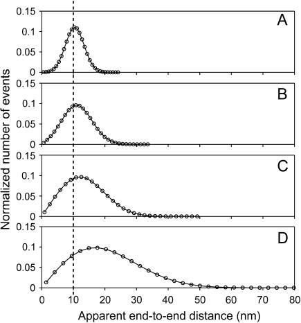
Fig. 1 shows an example of distance distributions and how they depend on the relative importance of the error on position measurements. Measured positions of two fluorophores separated by exactly 10 nm were Monte Carlo simulated, and the Euclidean distance between them was calculated. This was done a large number of times, and the distances measured in this manner were binned and plotted to obtain their distribution. When the signal/noise ratio (μ/σ) in distance measurements is good, the distribution is approximately Gaussian (Fig. 1 A). However as the signal/noise ratio decreases, the distribution becomes increasingly skewed as it broadens (Fig. 1, B–D), and the position of its maximum differs increasingly from the true distance between the fluorophores (Fig. 1, dotted line). If this were a real experiment and the binned data were fitted with a Gaussian whose central value were interpreted as the distance between the fluorophores, this distance would be grossly overestimated in Fig. 1 D. Even in Fig. 1 A, where the distribution looks reassuringly Gaussian, a 5% systematic overestimation would be introduced with a Gaussian approximation, as discussed below. This overestimation would be 13% and 32% for Fig. 1, B and C, respectively. Consequently, Fig. 1, A–C, represents the range of signal/noise ratios found in current single molecule localization experiments (1–4).

FIGURE 1.

Distribution of apparent distances for a given true distance, μ = 10 nm (dotted line), for four different values for the root mean-square deviation, σ, of the 2D Gaussian distribution of measured end-to-end vector differences. (Circles) Binned results from Monte Carlo simulations. (Curves) Graphs of p_2D(r) given in Eq. 4. The signal/noise ratios μ/σ in panels A–D are 3.33, 2, 1.25, and 0.667, respectively. A Gaussian analysis of these distributions would result in values that differ from the simulated value, μ, by 5% (A), 13% (B), 32% (C), and 112% (D). Note that although μ is kept fixed at 10 nm here for comparison to Fig. 3, simulations of different values of μ would yield the same functional forms assuming that the signal/noise ratio were kept the same, because p_2D(r) really depends only on and

The derivation of the function for proper treatment of data sets of distances in the plane goes as follows. Two different fluorophores, 1 and 2, with true 2D positions and then give rise to experimentally recorded positions and with Gaussian probability distributions

(1)

Here, is the variance in the fluorophores' location stemming from errors Gaussian distributed in the plane and (5). Consequently, is Gaussian distributed about with variance We wish to estimate from measurements of To this end, we write the Gaussian probability distribution for as a function of r and the angle φ between and

(2)

and integrate over a circle in the plane with radius r (Fig. 2, black dotted line) to obtain the probability distribution, p_2D(r), on the r axis in 2D,

(3)

The last integral is the modified Bessel function of integer order zero, I₀, so we have the result

(4)

The solid curves in Fig. 1, A–D, show graphs of this function for fixed μ and increasing values of σ. They describe the binned Monte Carlo simulated data of apparent distances precisely. This non-Gaussian distribution of distance measurements is not only the case for two dimensions. The distributions that replace p_2D(r) in one or three dimensions are, respectively,

(5)

and

(6)

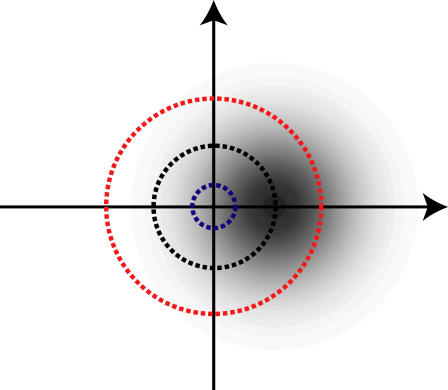
FIGURE 2.

A diagram to explain how a Gaussian distribution of apparent end-to-end vector differences integrates to the distribution of Euclidean distances given in Eq. 4.

Fig. 2 shows how the qualitative features in Eq. 4 arise. The distribution in shades of gray represents the Gaussian probability distribution for the vector difference between the two observed positions, assuming the first point is at the origin and the second is at a distance μ along the x axis. The three circles represent three different values of r along the distance axis. The corresponding probability distribution for apparent distances, p_2D(r), is obtained by integrating this Gaussian over all points a distance, r, from the origin, i.e., over circles centered on the origin. The three circles shown illustrate how the qualitative features of the apparent distance distribution come about. For the small blue circle the density of gray is almost constant across the circle. Consequently, the integrated probability for such a circle is proportional to its perimeter, and hence to its radius. Therefore p_2D(r) in Eq. 4 increases from zero value at zero distance in a manner that is proportional to distance for small distances, i.e., in a linear manner.

The black circle with radius μ passes through the point (μ, 0), which is where the vector difference has its probability maximum. However, the apparent distance distribution, p_2D(r), has its maximum at a larger distance, because a circle with larger radius (e.g., the red circle) has a longer section passing through densely gray regions of high probability, even though it does not pass through the point of maximal probability. For the same reason, yet longer apparent distances do have lower probability, but their probability density does not decrease as fast as a Gaussian function because their larger circles cut through larger parts of the Gaussian distributed vector difference. This is also the reason the apparent distance distribution decreases more slowly at large values of r than it increases at small values of r, i.e., why it is skewed.

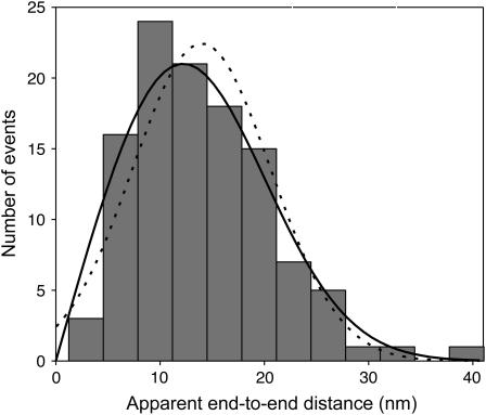
Fig. 3 shows a histogram of dsDNA apparent end-to-end distances measured using SHREC. The materials and methods involved to collect these data are as described (4). The distribution of these dsDNA end-to-end distance measurements (Fig. 3) is non-Gaussian. A maximum likelihood fit to the data with p_2D(r) in Eq. 4 (Fig. 3, solid line) results in an estimate for the end-to-end distance, μ, of 10 ± 1 nm and μ/σ of 1.3. This estimate for μ is in excellent agreement with the expected end-to-end distance of a 30 bp dsDNA molecule, assuming a 3.4 Å rise per base and a persistence length of 50 nm (6). A maximum likelihood fit with a Gaussian function is included for comparison (Fig. 3, dotted line) and yields the estimate for μ of 14 ± 0.5 nm. Although least-squares fitting to the histogram of data in Fig. 3 is inappropriate because of the low count in some bins, we did compute χ² of our maximum-likelihood fits after they had been done for the benefit of readers who find this quantity easier to judge than the statistical support of a fit. We found a reduced χ² of 1.7 of the p_2D(r) fit and 2.3 for the Gaussian fit. The Gaussian function, which above was mathematically proven to be the incorrect model for this experimental data set, expectedly fits the data less well and provides an estimator that is inaccurate. The correct measure of quality of our fits is the “goodness of fit” associated with all maximum-likelihood fits. For the p_2D(r) fit, we found the goodness of fit to be 68%. Details of the data analysis are provided in Appendix A.

FIGURE 3.

Histogram of apparent end-to-end distance measurements of dsDNA molecules (N = 112) determined by SHREC. The solid line represents the solution found when a maximum likelihood fit was performed with p_2D(r) given in Eq. 4. Goodness of fit is 68%. For comparison, the fit to the data with a Gaussian function is also shown (dotted line).

Even when σ² ≪ μ², in which case p_2D(r) in Eq. 4 can be approximated by a Gaussian function, the mean of this Gaussian is not a good estimate for μ. The maximum of p_2D(r) is not located at μ, but approximately at r = μ(1 + σ²/(2μ²)) (See Appendix B for details). So naively fitting data like those in Figs. 1 and 3 with a Gaussian function may result in an acceptable fit, depending on the noise in the data. Yet it will not yield the correct value for μ, but a systematic overestimation by a relative amount, σ²/(2μ²).

The p_2D(r) function (Eq. 4) appears to be sufficient to explain the 2D distance data sets arising from recent single-molecule fluorescent localization experiments. A number of researchers have fitted their data sets with Gaussian or lognormal functions with a constant background added to yield results closer to the data distribution's maximum (1–3). In these types of experiments it is unclear what would cause a uniform background in distance measurements. The skewness of the p_2D(r) distribution may provide an explanation for what previously has been perceived as a background.

CONCLUSION

It is natural to assume that a distribution of errors is Gaussian when it appears Gaussian by eye. However we conclude that by applying a Gaussian fit, one commits systematic errors on distance measurements with single-molecule fluorescence localization techniques. These techniques have overcome many technological hurdles to measure ever-shorter distances with high accuracy. The correct analysis of such data, as described here, ensures that the hard earned precision is not lost.

SUPPLEMENTARY MATERIAL

An online supplement to this article can be found by visiting BJ Online at http://www.biophysj.org.

APPENDIX A

The maximum likelihood fit was calculated in the following manner. Assuming a model such that P(x_i, a) describes the experimental data, one can calculate the probability that for a given set of estimators, {a_j}, a particular data point (x_i) occurs. Multiplying the probabilities of each data point gives the probability that the entire data set occurs with this set of estimators. The total probability is called the likelihood and is mathematically defined by the following equation,

The fit is found by numerically maximizing the likelihood (L) via varying the estimators, {a_j}(7).

Errors on the found estimators can be found by investigating the shape of the likelihood function along the axis of an estimator. Due to the central limit theorem, the probability distribution for each estimator, a_j, is a Gaussian function. To determine the error of an estimator, one needs to simply find the root mean-square deviation, σ, of the Gaussian likelihood function. In this article, errors were reported as being at σ from the maximum or at 68% confidence limits. In the online supplemental materials, we give a MATLAB (The MathWorks, Natick, MA) script that will automatically fit p_2D(r) in Eq. 4 to a data set and find the errors associated with the fit.

To test the significance of the maximum likelihood fit of p_2D(r) in Eq. 4 to the experimental data, a data set of the same size as the experimental data set (N = 112) was Monte Carlo simulated using the fit parameters {â_j} as input (as done to make the histograms in Fig. 1). The likelihood, L(x₁, …, x_N, â), was calculated and compared against the likelihood of the experimental data set. This was repeated a large number of times. The fraction of simulated data sets with a lower likelihood was 0.68, so the statistical support for the hypothesis that p_2D(r) is the correct theory for the data is 68%.

APPENDIX B

With our knowledge of p_2D(r) (Eq. 1), we can estimate the size of the systematic error that one commits if one interprets distance measurement data with a Gaussian function. The asymptotic expansion of the modified Bessel function is

so for σ² ≪ μ² we have a good approximation in

which looks similar to a Gaussian (8). However the factor is what makes p_2D(r) differ from a Gaussian function. This factor shifts the maximum of p_2D(r) to approximately r = μ(1 + σ²/(2μ²)). (Here we have ignored higher powers of σ²/μ²).

References

- 1.Gordon, M. P., T. Ha, and P. R. Selvin. 2004. Single-molecule high-resolution imaging with photobleaching. Proc. Natl. Acad. Sci. USA. 101:6462–6465. [DOI] [PMC free article] [PubMed] [Google Scholar]
- 2.Qu, X., D. Wu, L. Mets, and N. F. Scherer. 2004. Nanometer-localized multiple single-molecule fluorescence microscopy. Proc. Natl. Acad. Sci. USA. 101:11298–11303. [DOI] [PMC free article] [PubMed] [Google Scholar]
- 3.Balci, H., T. Ha, H. L. Sweeney, and P. R. Selvin. 2005. Interhead distance measurements in myosin VI via SHRImP support a simplified hand-over-hand model. Biophys. J. 89:413–417. [DOI] [PMC free article] [PubMed] [Google Scholar]
- 4.Churchman, L. S., Z. Okten, R. S. Rock, J. F. Dawson, and J. A. Spudich. 2005. Single molecule high-resolution colocalization of Cy3 and Cy5 attached to macromolecules measures intramolecular distances through time. Proc. Natl. Acad. Sci. USA. 102:1419–1423. [DOI] [PMC free article] [PubMed] [Google Scholar]
- 5.Thompson, R. E., D. R. Larson, and W. W. Webb. 2002. Precise nanometer localization analysis for individual fluorescent probes. Biophys. J. 82:2775–2783. [DOI] [PMC free article] [PubMed] [Google Scholar]
- 6.Hagerman, P. J. 1988. Flexibility of DNA. Annu. Rev. Biophys. Biophys. Chem. 17:265–286. [DOI] [PubMed] [Google Scholar]
- 7.Barlow, R. J. 1989. Statistics: A Guide to the Use of Statistical Methods in the Physical Sciences. John Wiley and Sons, New York.
- 8.Abramowitz, M., and I. A. Stegun. 1972. Handbook of Mathematical Functions. Dover Publications, New York.
Associated Data
This section collects any data citations, data availability statements, or supplementary materials included in this article.