Finding specific RNA motifs: Function in a zeptomole world?

Abstract

We have developed a new method for estimating the abundance of any modular (piecewise) RNA motif within a longer random region. We have used this method to estimate the size of the active motifs available to modern SELEX experiments (picomoles of unique sequences) and to a plausible RNA World (zeptomoles of unique sequences: 1 zmole = 602 sequences). Unexpectedly, activities such as specific isoleucine binding are almost certainly present in zeptomoles of molecules, and even ribozymes such as self-cleavage motifs may appear (depending on assumptions about the minimal structures). The number of specified nucleotides is not the only important determinant of a motif’s rarity: The number of modules into which it is divided, and the details of this division, are also crucial. We propose three maxims for easily isolated motifs: the Maxim of Minimization, the Maxim of Multiplicity, and the Maxim of the Median. These maxims together state that selected motifs should be small and composed of as many separate, equally sized modules as possible. For evenly divided motifs with four modules, the largest accessible activity in picomole scale (1–1000 pmole) pools of length 100 is about 34 nucleotides; while for zeptomole scale (1–1000 zmole) pools it is about 20 specific nucleotides (50% probability of occurrence). This latter figure includes some ribozymes and aptamers. Consequently, an RNA metabolism apparently could have begun with only zeptomoles of RNA molecules.

INTRODUCTION

The ability of particular RNA sequences to bind targets and catalyze reactions increases as the number of active sites grows with few apparent limits. Selection amplification, or SELEX (Ellington and Szostak 1990; Robertson and Joyce 1990; Tuerk and Gold 1990; Ellington et al. 2000), has revealed many novel reactions—carbon–carbon bond formation (Tarasow 1997; Sengle et al. 2001), amide bond synthesis (Lohse and Szostak 1996; Wiegand et al. 1997; Zhang and Cech 1997), acetyl-CoA synthesis (Jadhav and Yarus 2002), anhydride activation of carbonyl groups (Kumar and Yarus 2001), and aminoacyl-RNA synthesis both in cis (Illangasekare et al. 1995; Illangasekare and Yarus 1999a, 1999b) and in trans (Lee et al. 2000). This list could easily be lengthened.

However, assuming on this basis that RNA can do anything conceals a remarkable message from SELEX: Picomoles of random RNA molecules appear comprehensive. In other words, the fact that it is not unusual to find a new, arbitrarily chosen activity suggests that pools of the size typical for SELEX (10¹²–10¹⁵ molecules; random regions of 30–200 nucleotides) could contain nearly all chemically plausible RNA activities. Although infrequently emphasized, this is a profound result. If the number of random sequences needed for comprehensive pools were orders of magnitude greater, SELEX would be a far less successful endeavor.

Having established 10¹⁵ random sequences as a versatile RNA population, it becomes interesting to ask how few random sequences a pool can contain while remaining similarly comprehensive. More generally, how do the properties of the randomized pool affect the probability of finding a given RNA function? In particular, there has been a trend towards longer random regions and larger pools that are intuitively appealing, but not proven to be optimal.

One familiar aspect of SELEX is that only small pieces of a selected sequence are important; these short invariant sequences form the active site while large regions (e.g., stem-loops far from the active site) can be deleted with impunity. Biologic ribozymes share this characteristic of modularity. There are a few critical modules, which can often be identified from a multiple sequence alignment; between them, spacers may enforce certain structural requirements (such as a certain relative position) but have highly variable sequences. We use as examples the minimal isoleucine aptamer (Majerfeld and Yarus 1998) and the hammerhead ribozyme (Salehi-Ashtiani and Szostak 2001; Fig. 1 ▶): Both of these motifs have been isolated from SELEX, although the hammerhead is also found in organisms. The isoleucine site has two modules: a lower limit of 12 fixed nucleotides, and an upper limit of 18 fixed nucleotides. The hammerhead has three modules (including the paired region that contains the cleavage site): a lower limit of 11 fixed nucleotides, and an upper limit of 37 fixed nucleotides (the upper limit is given by counting as fixed those positions that conceivably could pair). Unexpectedly, the precise configuration of a motif (as well as the number of fixed nucleotides) is critical for predicting the difficulty of finding it in a random sequence.

FIGURE 1.

Examples of modular RNA sequences isolated from SELEX. Capital letters indicate initially random regions, while lower-case letters indicate fixed regions such as primer complements. Critical motifs are highlighted in bold. Diagrams at right show the motifs in their required structural context for the active site. Numbers in brackets indicate the position where the displayed sequence begins; ellipsis indicates that the sequence continues 3′ from the displayed region. (A) The minimal isoleucine motif (Majerfeld and Yarus 1998); although the conserved CUAC was originally found in the 5′ primer, subsequent reselection recovered this module from random sequence (S. Changayil and M. Yarus, pers. comm.), giving a total of 12 bases in two modules. If paired but otherwise unspecified regions are included, the site increases to 18 bases in two modules. (B) The hammerhead ribozyme, reselected from random sequence (Salehi-Ashtiani and Szostak 2001). The single U that comprises module 1 was supplied in a constant region; x marks the cleavage site. Thus, the hammerhead consists of 11 fixed nucleotides in three modules (the GC pair shown in plan text is conserved in natural hammerhead sequences, but was not recovered in SELEX). If paired but otherwise unspecified regions are included, this increases to 37 fixed nucleotides in three modules. Note that this upper limit is unrealistically large, because there are many possible sequences compatible with the required paired regions.

In this article, we build on previous work estimating the abundance of functional motifs in random pools (Ciesiolka et al. 1996; Lorsch and Szostak 1996; Sabeti et al. 1997; Yarus and Knight 2002). We estimate the systematic effects of the length of the random region, the length of the motif, and the division of the motif into modules with crucial fixed sequences. We ask how frequently motifs should occur in particular types of random pool, using the isoleucine aptamer and the hammerhead as examples. In particular, we assess the largest motifs that would be expected to occur in the picomole-scale pools used in SELEX, and in the zeptomole-scale (1 zmole ≈ 602 sequences to 1000 zeptomoles ≈ 602,000 sequences) pools that might be more plausible during the origin of RNA-catalyzed metabolism.

RESULTS

The number of ways to find a short motif in a longer sequence grows dramatically as it is divided into an increasing number of separate modules, and also as the length of the randomized sequence to be searched increases (Fig. 2 ▶; Sabeti et al. 1997; Yarus and Knight 2002).

FIGURE 2.

Number of spacer divisions D as a function of spacer length s and modularity m. Modularity ranges from 1 to 6; each label refers to the line above it. Note logarithmic scale on the y-axis. The number of divisions increases very rapidly at high modularity: for example, there are more than 100,000 ways to divide 40 bases of spacer among four modules.

Our new calculation (see Materials and Methods) shows quantitative agreement with simulations that directly count all possible motifs in computer-generated random sequences; however, it has the advantages that it eliminates sampling error and takes seconds rather than days to finish on a desktop computer. Figure 3 ▶ shows the fit between the model (lines) and the simulations (symbols). The computation (Materials and Methods) provides accurate predictions for all sequence lengths, motif lengths, and divisions into modules tested, although sampling error for individual sequences can be high when the sequence length is short (scatter in points towards the left of Fig. 3 ▶). These sampling effects disappear when the random region is longer than about 50 nucleotides; in any case, the deviations from predictions are insignificant when examining the means of results from 25 independently simulated sequences.

FIGURE 3.

Agreement between calculations and simulations. The number of unique motifs (i.e., sequences that differ in at least one module, y-axis) grows dramatically as the sequence length, x-axis, and modularity grow, although not as fast as does the number of trials (cf. Fig. 2 ▶). Lines are the results of the calculations as derived in Materials and Methods; dots are 25 runs of simulations in which randomly generated sequences were divided into modules in every possible way for a given length and configuration. Dark lines denote evenly divided motifs (e.g., [5,5,5,5] represents a motif of 20 divided into four equal modules); light lines denote unevenly divided motifs (e.g., [17,1,1,1] represents a motif of 20 divided into four modules in which the difference between the largest and smallest modules is as great as possible). Note the dramatic effect (orders of magnitude) of unequal division of the motif. The spread of the dots (each from an individual random sequence) gives an idea of the sampling error: large for short sequences and high modularity; very low once the sequence reaches 60 nucleotides. The model gives excellent agreement with the simulations over a wide range of modularity, sequence length, and size of individual modules. It is impractical to collect simulation data for longer sequences due to the running time (approx. 6 h and 500 MB RAM for modularity 4 and sequence length 100 on a 1.8 GHz Pentium 4; more than 4 d and 4 GB RAM/swap space for sequence length 200).

In the following discussion, we use the notation [x, y, …] to denote the division of a motif into modules of different sizes. For example, [10, 10] indicates a motif of total length 20 divided into two equal 10-nucleotide modules, while [1, 9, 3, 7] denotes the same motif divided into four unequal modules of length 1, 9, 3, and 7, respectively. When all modules are fairly large, nearly every combination of positions in the sequence should give a new motif. Consequently, when the motif is evenly divided into modules that are about the same size, the number of unique motifs found in each sequence is about equal to the number of trials. However, for unevenly divided motifs (e.g., dividing a motif of length 20 into [17, 1, 1, 1] rather than [5, 5, 5, 5]), there is a dramatic decrease in the number of distinct motifs found. The reason for this is that the short modules are so easily found. For example, dividing the motif into [19, 1], each starting position along the sequence is likely to yield a new 19 mer, but there are only four possibilities for the monomer. Consequently, the total number of unique motifs cannot be more than four times the number of positions for 19 mers. In contrast, dividing the same motif evenly into [10, 10], nearly every starting position will yield a new state for both modules. Thus the total number of unique motifs can grow very rapidly.

Accordingly, the division into modules has a surprisingly large effect on the number of random sequences that must be searched to find a motif of a given size. Figure 4 ▶ shows this effect for different ways of dividing a motif with 15 fixed nucleotides divided among three modules, ranging from the most equal [5, 5, 5] to the most unequal [13, 1, 1] divisions. For longer sequences, division can make several orders of magnitude difference to the probability of finding the motif in a single sequence, and hence, in the required pool size. The effect is even greater for longer motifs and higher modularities; we use this case as an illustration because the number of different ways of dividing the motif is still (relatively) manageable at 91. Note also that many such 15 nucleotide motifs are expected in a pool containing only zmoles of RNA.

FIGURE 4.

Importance of evenly divided modules. Individual lines show different divisions of a 15-nucleotide motif into three modules. For a random region of 100 nucleotides, only 51,000 molecules would need to be searched to have a 99% chance of finding a motif divided into three 5 mers (heavy line at bottom of graph), but nearly four million molecules (a factor of almost 100) would need to be searched to have the same chance of finding a motif divided into a 13 mer and two monomers (heavy line at top of graph). The other lines show the other 87 ways of dividing the motif. Out of 91 total ways, there is one way to divide it into three 5 mers, there are three ways to divide it into a 13 mer and two monomers: [13, 1, 1], [1, 13, 1], and [1, 1, 13]. Similarly, there are three ways to divide it into any other configuration in which two of the pieces are equal. There are six ways to divide it into any particular configuration where all three pieces are unequal: for example, [9, 4, 2], [9, 2, 4], [4, 9, 2], [4, 2, 9], [2, 9, 4], and [2, 4, 9]. Only the size of the pieces, not their order, affects the probability, so only 19 distinct lines are visible on the graph (some are very close together). The top two lines on the graph (the [13, 1, 1] family and the [12, 2, 1] family) are clear outliers; most divisions are closer to the best case of [5, 5, 5] than to the worst case. This effect becomes more extreme at higher modularity. The horizontal gray bar shows 1000 zeptomole (602,000 sequences).

We can now calculate the pool sizes that would be necessary for finding new instances of the isoleucine aptamer and the hammerhead ribozyme (Fig. 1 ▶). Although we will address the problem of finding structure motifs (that is, correct folds) in a future article, here we are concerned only with the presence of the underlying sequence motifs. For the two-module isoleucine site, the lower limit for the essential nucleotides is [4, 8] counting only absolutely conserved nucleotides, while the upper limit is [7, 11] when counting nucleotides in the helices also—an average of [5, 10] or [6, 9] (because there is an odd number of pairs) might be most reasonable. For the three-module hammerhead site, the lower limit is [1, 6, 4] and the upper limit is [10, 14, 13]—the average is [6, 10, 9] or [7, 10, 8] (because there is an odd number of pairs between modules 1 and 3). Figure 5 ▶ shows that the isoleucine aptamer is likely to be found in very small pools of RNA (tens to hundreds of thousands of molecules), as also may the hammerhead, although this probability depends on assumptions about the paired regions.

FIGURE 5.

Pool sizes required to find the isoleucine aptamer (black) and the hammerhead ribozyme (gray) (Fig. 1 ▶), making different assumptions about sequence requirements. The horizontal gray line represents 1000 zeptomoles, the limit of the Zeptomole World. The isoleucine aptamer is almost certainly a Zeptomole World molecule; the hammerhead may or may not be, depending on how much helix is added to its required sequences. However, its essential sequence components should certainly appear in zeptomole-scale pools. Thin lines show the minimal sites (fixed sequence only); dark lines show the maximal sites (counting paired bases as fixed in one state); and medium lines show the average (counting half the paired bases as fixed; details in how the paired bases are assigned are not visible on this scale). The graph shows pools required for 50% probability of occurrence; for 99% occurrence, multiply all pool sizes by a factor of 6. The maximal sequence for the hammerhead is clearly not a realistic case, or it would not be possible to reproducibly recover this motif from SELEX.

Finally, we calculate the largest motifs accessible to modern SELEX and to a zeptomole world. Figure 6 ▶ shows the relationship between motif size and number of sequences required for 50% probability of finding the motif, for random regions of length 40, 80, and 120. Although the length of the random region has a significant effect, the largest effect is from increase in the number of modules. Figure 7 ▶ shows the largest motifs accessible in zeptomole-scale (600,000 sequences) and SELEX-scale (10¹⁵ sequences) random pools as a function of sequence length. Zeptomole-scale pools can probably access motifs of about 20 nucleotides (random region of length 100) at modularity 4, and about 18 nucleotides at modularity 3. SELEX-scale pools should be able to access motifs of about 26 nucleotides (random region of 40, modularity 1) to 34 nucleotides (random region of 100; modularity 4). These results are comparable to the number of essential nucleotides and modularities of many actual RNA activities. Further, the number of accessible nucleotides agrees with our previous calculation by another method (Yarus and Knight 2002), although those prior calculations count all configurations of a motif and the present numbers are only the leading terms (for evenly divided motifs; cf. Maxim 3 below). In addition, because the present calculations agree with prior independent results at both zmole and pmole levels, the rule of 1.66 nucleotides added to the motif/10-fold increase in RNA (Yarus and Knight 2002) is also confirmed by these new calculations as the limiting case (see Fig. 6 ▶).

FIGURE 6.

Number of sequences required to find evenly divided motifs in random pools of (A) length 40, (B) length 80, and (C) length 120, for modularities of 1 to 4. Results shown for 50% probability of occurrence; for 99%, multiply all pool sized by a factor of 6. Horizontal dark line indicates 1000 zeptomoles. x-Axis shows total length of motif; y-axis shows number of molecules required.

FIGURE 7.

Largest accessible evenly divided motifs in (A) zeptomole-scale pools, and (B) SELEX-scale pools (602,000 and 10¹⁵ sequences, respectively). X-axis shows length of the sequence; y-axis shows largest motif accessible for each modularity at probability 0.5 (increasing the probability to 0.99 decreases the length of the accessible motif by at most two nucleotides in this range).

DISCUSSION

Our new model for predicting the abundance of motifs gives quantitative agreement with simulations of actual sequences (Fig. 3 ▶), and is also in substantial agreement with prior estimates. Hence, we feel confident in using it to predict the frequency of sequence motifs in random pools far too large to simulate directly. Assuming that motifs will be recovered from SELEX (or appear by natural selection) in proportion to their initial abundance, we infer the following maxims about RNA sequences likely to be selected.

Maxim of minimization

Selected motifs will be as short as possible. Each additional fixed nucleotide makes the motif approximately a factor of 4 rarer (requiring fourfold more RNA to have an equal chance of finding it; the 1.66 nucleotide rule), and this applies exactly in the limit of long, evenly divided modules and large pools. For tiny possible primordial motifs, the cost of adding an additional base can be considerably less. In any case, small motifs will always be markedly more abundant.

Maxim of multiplicity

Abundant motifs will be divided into as many pieces as possible. This maxim must observe the requirements for structural stability. Although a motif made up of 12 single nucleotides scattered through the sequence would be very easy to “find”, it is highly unlikely to fold correctly. However, modules containing only a single absolutely required base are often important (for instance, the U next to the cleavage site in the hammerhead ribozyme). We hope to use computational folding methods to assess the apparent relationship between stability and function in more detail.

Maxim of the median

Most probable motifs will be divided as evenly as possible. In other words, it takes far more random sequences to find a motif of 20 divided into [17, 3] than when divided into [10, 10]. In fact, the evenness need only be approximate to give almost the same probability of occurrence (i.e., [12, 8] is not notably worse than [10, 10]), but extreme inequality of division would suggest selection for specific functional consequences (because unequally divided motifs are fundamentally harder to find than more evenly divided ones).

In addition, we can assess the effect of pool size and random region length on the largest accessible motifs. Increasing the pool size has a relatively minor effect; when modules are relatively large, each 10-fold increase in the number of sequences provides only an additional 1.66 nucleotides to the length of the random region (Yarus and Knight 2002). This region is that of parallel lines in Figure 6 ▶ (slope = 1.66 nucleotides/order). As can be seen in the figure, evenly divided motifs in pools having more than 100 molecules (a few tenths of a zeptomole) obey the rule, which is therefore quite general. Figure 7 ▶ shows that increasing the number of sequences from 602,000 to 10¹⁵ roughly doubles the length of the accessible motif; thus, to increase this length by another 50% would require another 10 ⁹-fold increase in the amount of RNA, or about 33 kilograms of RNA in a volume of 100,000 liters. The converse of this is that surprisingly large and complex RNA activities may have been available very early in evolution (for further discussion, see Yarus and Knight 2002).

A more efficient method of increasing the chance of finding a motif is to increase the length of the random region: For zeptomole pools, going from 30 to 200 increases the accessible motif (of modularity 4) by eight nucleotides. Thus, less than a sevenfold increase in the length of individuals yields the same effect as a 66,000-fold increase in the number of sequences. The importance of the length of the random region increases somewhat as the number of sequences increases: For SELEX-scale pools, the same 170-nucleotide increase in length increases the accessible motif by 10 nucleotides. However, although longer random regions are more likely to contain the required sequences, they are also more likely to find alternative stable folds that do not bring the modules together into the correct structure (Sabeti et al. 1997). We are investigating this latter effect quantitatively, because it is likely to be crucial for the efficiency of SELEX experiments.

CONCLUSIONS

We have devised a new method for calculating the probability of finding a set of short modules within a longer sequence. We have used this method for assessing the capabilities of the picomole-scale pools used in SELEX as well as the zeptomole-scale pools that might have been more relevant to the origin of RNA metabolism. By bridging two very different scales of selection we can ask which of the findings of SELEX could also apply to the RNA World.

Surprisingly, we find that the number of fixed nucleotides required for a motif is not the only factor that affects its abundance: The number of modules, and also the evenness with which the motif is divided among them, are also critical. Although the length of the random region and the pool size do have a significant effect on the largest motifs that can be selected, unexpectedly tiny pools of randomized RNA appear likely to contain significant functionality. The abundance of different motif configurations suggests that, as much as possible, both natural and artificial selection should favor sites with as many small, evenly divided modules as possible.

Here we have only focused on the probability of finding the right sequence for activity; we hope also to address the probability of finding the right structure. Because we can now calculate the probability that a random region contains the correct sequence, we can sample from these sequences directly and use folding algorithms to obtain insight into the distribution of RNA activities. In particular, we suspect that longer sequences are decreasingly likely to fold correctly, which would decrease the benefits of longer randomized sequence length compared to the calculations presented here.

The mathematical framework we have developed should be applicable to assessing the frequency of other types of modular sequences. For instance, it could be used to calculate the probability that a set of transcription factor binding sites occurs in the correct order within a given distance from a transcription start, or the probability that a set of “signature” amino acid sequences occurs in a putative new member of a protein superfamily. Such statistics may allow more precise discrimination of real functional sites from chance occurrences.

Finally, we predict that we will be able to isolate ribozymes and aptamers from real pools containing 1–1000 zeptomoles of unique sequences. If the advantages of modular folds indeed make functional RNA molecules so accessible, the RNA World becomes almost inevitable (Yarus and Knight 2002).

MATERIALS AND METHODS

Number of divisions of a sequence into modules

One critical question for determining the probability of a sequence match is how many ways there are to find a short, modular motif in a longer sequence. Previous calculations of this quantity have either been approximate (Sabeti et al. 1997) or required estimated sampling corrections (Yarus and Knight 2002). Here, we provide a potentially more transparent method (Fig. 8 ▶).

FIGURE 8.

Calculations for D, the number of ways of dividing a sequence to look for a set of shorter modules. First, partition the number of bases in the sequence n into the number of bases in modules, l, and the number of bases in spacer, s = (n − l). Each possible position of the modules within the longer sequence can be thought of as a particular way of choosing m places to cut the spacer, with the provisions that two cuts cannot occur in the same place and that one cut can occur after the last base of the spacer (i.e., the last module can be at the 3′ end of the sequence). However, the order in which the m cuts are chosen does not matter (even if the cut for the last module was made first, the modules will still be looked for in order). Thus, D is equal to the number of ways of choosing m items from s + 1.

An RNA sequence is divided into functional modules and intercalated nonfunctional spacer elements. Let the total length of the sequence be n nucleotides, the sum of the lengths of the modules be l, and the number of separated modules be m. Then the number of nucleotides in the spacer s is (n − l).

By definition, each module must be separated from its neighbors by at least one nucleotide of spacer. Consequently, the problem is equivalent to finding the number of ways to cut the s nucleotides of the spacer m times while leaving a gap of at least one nucleotide between cuts. Because modules are allowed to appear at the ends of the sequence, there are s + 1 positions at which a cut could occur—before each of the s nucleotides of the spacer, and at the end of the molecule (Fig. 8 ▶). Thus, there are (s + 1) ways to make the first cut, that is, to insert one module. If there is a second module, it can be inserted anywhere except at the same position as the first module (or the modules would be adjacent): Thus, there are s ways to make the second cut, s − 1 ways to make the third cut, and, in general, s − (m − 1) ways to make the m^th cut. Because the cuts are independent, the number of possibilities is given by (s + 1) × (s) × (s − 1) × … × (s − (m − 1)), or (s + 1)!/(s − (m − 1))! However, the order of the cuts is unimportant because the modules are always inserted in the same relative positions; for example, choosing positions 1, 2, and 3 is the same as choosing positions 3, 1, and 2. Because there are m cuts, we must divide by an additional factor of m! to reflect the number of ways of making the same cuts. Thus, D, the number of ways of dividing the spacer (and, hence, the number of possibilities for finding a particular combination of modules within a given molecule), is:

D is the well-known binomial coefficient, giving the number of ways of choosing m things from s + 1. D increases extremely rapidly both with the length of the spacer and the number of modules (Fig. 2 ▶). For a single module, D = s + 1. Consider, for example, an 80-nucleotide random region with a 20-nucleotide motif (and, consequently, 60 bases of spacer). If the motif consists of a single 20 mer, there are 61 chances for it to match. In contrast, if the 20-mer motif consists of four critical 5-mer modules, there are nearly a million chances for it to match. Because the total number of possible sequences in each case is the same (4²⁰ ≈ 10¹²), it is clear that far fewer random 80 mers need to be searched to find a given divided motif than an undivided one the same size (Yarus and Knight 2002).

Two numbers determine D: the number of modules, and the number of possible positions that each module can take. These we call the dimension and the size of the problem, respectively. The size of the problem, which we label z, represents the maximum number of positions that a module could experience across all the possible ways of arranging the remaining modules, and is the same for every module. The reason for this is straightforward. Consider two examples. First, for a module to be in its left-most position, the first module must occur at the start of the sequence and all modules between the first module and the module under consideration must be separated by a single base of spacer. Thus, the first position at which the module could start is the sum of the lengths of all the modules to its left, plus one base of spacer for each of these modules, plus 1 (if the first base is counted as base 1 instead of base 0). Second, for a module to be in its right-most position, the last module must occur at the end of the sequence and all modules between the last module and the module under consideration must be separated by a single base of spacer. Thus, the last position at which the module could end is the sum of the lengths of all the modules to its right, plus one base of spacer for each of these modules, subtracted from the length of the molecule. To get the last position at which the module could start, subtract one less base than its length from the position at which it ends (because the end position takes up a base). In fact, no matter which module is under consideration, the total number of bases left over for it to slide along is the length of the sequence, minus the sum of the lengths of all the modules (including the current module), minus one base for all the modules except the last module (because no spacer is needed after the last module), plus one base for the fact that the numbering begins at 1. Thus, the size z is equal to (s + 1) − (m − 1), or (s − m + 2).

This concept of the size of the problem (in terms of the number of positions each module could occupy) is critical for understanding the probability calculations that follow. For a problem of a given size and dimension (i.e., amount of spacer and number of modules), the number of possibilities is the sum of all the problems up to the same size in one fewer dimension. This is because the maximum number of positions for the second module (and all subsequent modules) is the size of the original problem, but, as the first module slides along to the right, there are progressively fewer bases of spacer left over for the remaining modules to slide around in. Because the spacer is divided in all possible ways among the remaining modules, this is equivalent to solving successively smaller problems in one fewer dimension, from z down to 1 (the case where there is no spacer left over). Figure 9 ▶ shows this relationship in problems of size 1 to 4 with dimensions 1 to 3. Each module can only occupy a certain number of positions as it moves along the sequence, and many positions are mutually exclusive. For example, in the case where m = 2, when the first module is in its rightmost position, there is only one position (at the very end of the sequence) where the second module could be found, but when the first module is in its left-most position the second module could be found in any of three additional positions.

FIGURE 9.

Dependence of the number of positions each module can take on the number of modules m and the size of the problem z. The top line in each block shows all the positions that each module can occupy. Each subsequent line in the block shows a single valid position for each module (dark dashes, numbered according to module), along with the possible alternative positions for the last module (light dashes). This highlights the fact that the successive left-most positions of the last module correspond to successive sizes of the one-dimensional problem. Note that to keep the size constant it is necessary to add another spacer position for each additional module. The Current column shows the number of positions contributed by the current size of the (m − 1) dimensional case, while the Sum column shows the total number of positions for the current size of the m-dimensional case. Horizontal arrows show the contribution of each new term (larger size) to the sum: adding a base of spacer is the same as adding the case with the new number of bases of spacer in one lower dimension. Horizontal and vertical arrows show that each successively larger term in a given dimension is the sum of the previous term in that dimension and the larger term in one fewer dimension. Oblique arrows show the relationships between terms in successive dimensions.

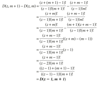
It is possible to calculate explicitly the effect of incrementing the size (adding one to the spacer length while keeping the number of modules constant), and of incrementing the dimension (adding another module while keeping the spacer length constant). Incrementing the size is equivalent to adding the next larger case in (m − 1) dimensions. In other words, the number of possible combinations that are added by adding a base to the spacer is equivalent to finding the number of ways to distribute the new, larger spacer among all modules except the first (because for the remaining modules to see the additional base, the first module can only occupy its left-most position). Incrementing the dimension is equivalent to adding the next smaller case in (m + 1) dimensions, which is the same as the sum of all smaller cases in the current dimension. That is, the number of combinations added by adding a module and its required base of spacer to the sequence is equivalent to finding all the ways that the current number of modules could be arranged in smaller amounts of spacer (because the amount of spacer to be distributed among these modules decreases as the new module slides along to the right). These identities, which are shown geometrically in Figure 10 ▶, can also be shown algebraically as follows.

FIGURE 10.

Effect of increasing the size or dimension of the problem. Starting with the case where z = 3 and m = 2, incrementing z to get D(4,2) is equivalent to adding D(4,1); In other words, the next larger case in one less dimension (top). Conversely, incrementing m to get D(3,3) is equivalent to adding D(2,2) and D(1,2) (side: left of arrow). This is equivalent to adding D(2,3) (because a given term in d dimensions is the same as the sum of all terms up to that size in d − 1 dimensions as shown in Fig. 9 ▶); in other words, this is the same as adding the next smaller case in the same number of dimensions (side: right of arrow).

Incrementing the size

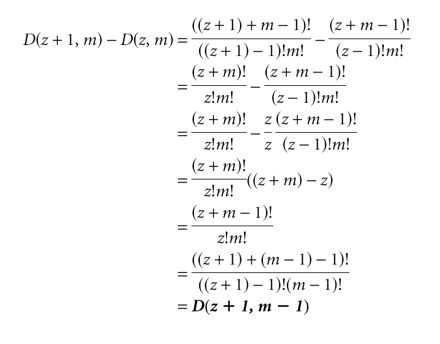
Incrementing the dimension

The Poisson approximation

Having calculated the number of ways of searching for a motif in a longer sequence, we now need to calculate the probability that a sequence picked at random contains the motif. If the probability that a module matches at a particular position is fixed (p = 4^−l for random sequences with unbiased base composition), the mean number of times that the module matches in a given sequence is simply D × p. Consider the case of a random region of length 80 and a motif length of 8, divided into two modules. The probability of observing a match on any one trial is 4⁻⁸ or 1.53 × 10⁻⁵, the number of chances to match in each molecule is D(72,2) or 2628. Consequently, the mean number of matches in a single molecule is 0.04. If we assume that matches follow a Poisson distribution, the probability of not finding a match in a single molecule would be e^−0.04 or 0.96; consequently, it would be necessary to examine about 115 molecules to have a 99% chance of finding a match (0.96¹¹⁵ ≈ 0.01). This number would be the same no matter how the motif was divided into two modules (i.e., [4, 4] would be the same as [7, 1]).

However, the Poisson approximation is inaccurate because successive trials are not independent: The same parts of the sequence are resampled many times and combined with other modules. Figure 11 ▶ shows the deviations from predictions for different way of dividing a motif of length 8. When the motif is divided into [4, 4], simulation shows there is over a 99% chance of finding it in 150 sequences (the prediction of 115 sequences assuming independence above is optimistic). If, on the other hand, the motif is divided into [7, 1], even 500 sequences are insufficient to be 90% confident of finding it, and it would take over 1100 sequences to reach 99% probability. When all ways of dividing the spacer are considered together (solid line), the probability of finding a motif in N sequences cannot even be projected from the results for a single sequence. This is because the sum of multiple exponential decay curves is not itself exponential, and so the predictions are very different in different parts of the curves (dashed line). In particular, at the beginning the slope of the overall curve is the same as the single-sequence extrapolation. However, as the number of sequences increases, the slope converges to that of the most elusive motif (lowest slope). This curve is vertically offset by a constant factor that represents the fraction of all configurations contained within this most slowly found class.

FIGURE 11.

Violation of Poisson sampling assumptions. Dividing a motif of constant modularity into pieces affects the number of sequences that need to be searched to minimize the probability that a motif will be missed (logP, y-axis: logP[not found] of −2 is equivalent to a 99% chance that the motif is found). The vertical line at 115 sequences is the Poisson prediction for a 99% chance of finding an 8 mer divided into two pieces in a random region of length 80. Thin solid lines show the progression for the fastest-changing [4,4] and slowest-changing [7,1] and [1,7] configurations: independent sequences have a constant probability of finding each motif, and so the relationship is log-linear. The thick solid line shows the probability of missing a sequence when all configurations of the motif (all divisions into two modules) are combined: the nonlinearity shows that the results for a single sequence do not scale to multiple sequences, because different configurations saturate at different rates. This line is derived from two runs of the simulation (diamonds and crosses). Dashed lines show extrapolation for the combined configurations either from the results for a single sequence (steeper slope) or from 500 sequences (shallower slope). Note the large discrepancy (two orders of magnitude) between the projection from a single sequence and the actual results for a sample of 500 sequences.

The explanation for the decreasing slope is relatively straightforward: Although the number of different combinations is very large, each module only occurs in a few different positions. This number of positions is equivalent to z, the size of the problem, defined above as (s − m + 2). For the case of a modularity of 2, motif length of 8 in a sequence of 80, each module experiences (80 − 8 − 2 + 2) or 72 different positions. If the motif is divided into [4, 4], so that each module has 4⁴ or 256 possible states, we expect most of the 72 positions to represent different sequences. If, on the other hand, the motif is divided into [7, 1], so that the first module has 4⁷ or 16,384 possible states while the second module only has 4¹ or 4 possible states, even though all 72 of the positions for the first module are likely to represent different sequences the second module will sample each of the four bases many times. Thus, the largest possible number of distinct motifs in the sequence is (72 × 4) = 288—much smaller than the 2628 motif combinations calculated above. Conversely, the motifs that do occur are found an average of nearly 10 times each. Although the mean number of occurrences per sequence is the same for both cases, the variance is much higher with uneven divisions and far more sequences have to be searched before the motif is likely to be found.

Accounting for sampling

The Poisson approximation is inaccurate because combinatorial attempts at matching the motif reuse the same few positions for the individual modules (Yarus and Knight 2002). It is possible to avoid this effect by explicitly calculating the probability that, given the positions of the first (m − k) modules, there is a configuration of the remaining k modules such that all of the modules match their corresponding target sequence. The key here is to consider the position of each possible match, weighted by its probability of occurrence.

A sequence contains a complete match if and only if the target sequence for each module is present, and then only if the target sequence for each module occurs to the right of the target sequences for each of the preceding modules. Thus, we are always concerned with the left-most allowed match for each module, where an allowed match is one that occurs to the right of the last match in the previous module. Note especially that the position of the left-most allowed match determines the number of bases of spacer that can be distributed among all the subsequent modules, and hence, the size of the subproblem that needs to be solved to calculate the probability of the subsequent matches.

For a single module, the probability that the first position is the left-most match is simply p, the probability of a match in a single trial, defined above as 4^−l where l is the length of the current module. The probability that the second position is the left-most match is somewhat lower: p × (1 − p), or the product of the probability that the second position is a match (p) and the probability that the first position was not a match (1 − p). Each additional position to the right incurs an additional factor of (1 − p), because, for a position to be the left-most match, all positions to the left of that position must have failed to match. Thus, the probability that each position is the left-most match forms a geometric series, p, p(1 − p), p(1 − p)², … , p(1 − p)^z−1, where z is the size of the problem (i.e., the number of distinct positions that the module could potentially occupy).

The probability that the single module matched at least once is equivalent to the probability that one of the z positions was the left-most match. This is given by the sum of the geometric series with starting term p, and ratio (1 − p). Substituting into the standard formula for the sum of a geometric series (a(1 − r)ⁿ/(1 − r), where a is the starting term, r is the ratio, and n is the number of terms), we obtain:

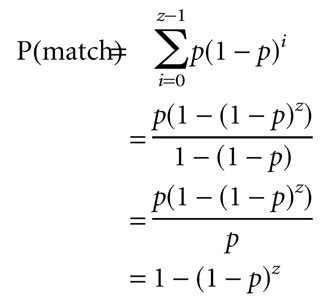
This can be checked by comparison with the probability that there is no match in the sequence, which is (1 − p)^z (i.e., the probability that a particular position fails to match raised to the power of the number of possible positions). Because there must either be no match or at least one match, these two probabilities sum to 1; this count of matches is exhaustive.

Having determined the probability for a matching single module, we now extend calculation to arbitrary numbers of modules (Fig. 12 ▶). Again, the size of the problem is given by z = (s − m + 2), and the dimension is given by the number of modules m. For the left-most module, the probabilities that there is a match at the first, second, third, etc., possible positions are given by the one-dimensional case. The number of spacer positions left over determines the size of the (m − 1)-dimensional problem that needs to be solved to determine the match probabilities for the remaining modules. Consequently, the problem can be solved in m dimensions by solving the problem for all possible sizes in (m − 1) dimensions and weighting the probability of each subproblem by the corresponding probability that the position leading to it was the left-most match.

FIGURE 12.

Probability of matching a set of modules. Example cases as for Figure 4 ▶, but note change in numbering (positions are now relative to the first position that the module can occupy under any circumstance, rather than relative to the first position that it can occupy relative to the positions of the other modules in the current case). The top line in each set shows the left-most position each module can take (given a particular state of the first module), and hence, the left-most possible match for each module. The position of the left-most match for the first module determines the size of the problem to solve for the remaining modules (in one fewer dimension). P_n is the probability of a match in the nth module; Q_n = (1 − P_n). For m = 1 (top), the probability of a match at the ith position is P₁Q₁^{(i − 1)}. For m = 2 (middle), the probabilities for the first module remain the same; however, depending on the position, a different size subproblem must be solved in one dimension to find the probability that the second module also matched. Similarly, for m = 3 (bottom), the position of the left-most match of the first module determines the size of the two-dimensional subproblem that needs to be solved to find the probability that all three modules matched. In general, to solve for m modules, it is necessary to solve all smaller problems in (m − 1) dimensions, and to weight each of these solutions by the probability that the first module matched in a position compatible with it. The diagrams to the right show the probabilities of each of the allowed combinations of positions (order the same as the ordering of the lines to the left); to find the probability that a particular combination was the left-most set of matches (e.g., first module at its second position, second module at its second position, third module at its fourth position), multiply the individual terms together (here, P₁Q₁ × P₂ × P₃Q₃², as can be seen either by examining the individual line corresponding to this case or by examining the relevant cell in the table). Arrows show the correspondence of terms in lower dimensions as parts of higher dimensional problems.

This progression provides an efficient way of computing the overall solution. Instead of calculating the probability of each possible module configuration directly (which would scale exponentially with the number of modules), the following algorithm reduces the calculation to linear in the number of modules and quadratic in the number of bases of spacer. The algorithm follows the flow of Figure 12 ▶, in which all successively smaller subproblems of a given dimension appear as terms in the calculation of the next dimension (weighted by the probability that there are that many bases of spacer left over for the remaining modules).

Initialization

Fill array current_dimension of size z with the one-dimensional case representing first module:

p₁, p₁(1 − p₁), p₁(1 − p₁)², …

Replace the terms of current_dimension with cumulative sums to get the probabilities of having found the module:

p₁, p₁ + p₁(1 − p₁), p₁ + p₁(1 − p₁) + p₁(1 − p₁)², …

current_dimension now holds solutions for all sizes of the one-dimensional case for the first module.

Loop

Fill array last_dimension with the values of current_dimension

Empty current_dimension

Fill array coefficients of size z representing the one-dimensional case for the current dimension

Reverse order of coefficients

While coefficients is not empty:

Set variable sum to zero

For each item in coefficients:

Find corresponding item in last_dimension

Multiply these two items and add to sum

Add sum as a new element at the start of current_dimension

Delete first element of coefficients

current_dimension now holds the first n terms in the current dimension.

Return

Last element from current_dimension

Perl programs implementing this algorithm, and an algorithm that tallies the number of unique motifs found when searching random sequences for a particular motif configuration, are available on request from the authors.

REFERENCES

- Ciesiolka, J., Illangasekare, M., Majerfeld, I., Nickles, T., Welch, M., Yarus, M., and Zinnen, S. 1996. Affinity selection-amplification from randomized ribooligonucleotide pools. Methods Enzymol. 267: 315–335. [DOI] [PubMed] [Google Scholar]
- Ellington, A.D. and Szostak, J.W. 1990. In vitro selection of RNA molecules that bind specific ligands. Nature 346: 818–822. [DOI] [PubMed] [Google Scholar]
- Ellington, A.D., Khrapov, M., and Shaw, C.A. 2000. The scene of a frozen accident. RNA 6: 485–498. [DOI] [PMC free article] [PubMed] [Google Scholar]
- Illangasekare, M., Sanchez, G., Nickles, T., and Yarus, M. 1995. Aminoacyl-RNA synthesis catalyzed by an RNA. Science 267: 643–647. [DOI] [PubMed] [Google Scholar]
- Illangasekare, M. and Yarus, M. 1999a. Specific, rapid synthesis of Phe-RNA by RNA. Proc. Natl. Acad. Sci. 96: 5470–5475. [DOI] [PMC free article] [PubMed] [Google Scholar]
- Illangasekare, M. and Yarus, M. 1999b. A tiny RNA that catalyzes both aminoacyl-RNA and peptidyl-RNA synthesis. RNA 5: 1482–1489. [DOI] [PMC free article] [PubMed] [Google Scholar]
- Lee, N., Bessho, Y., Wei, K., Szostak, J. W., and Suga, H. 2000. Ribozyme-catalyzed tRNA aminoacylation. Nat. Struct. Biol. 7: 28–33. [DOI] [PubMed] [Google Scholar]
- Lohse, P.A. and Szostak, J.W. 1996. Ribozyme-catalysed amino-acid transfer reactions. Nature 381: 442–444. [DOI] [PubMed] [Google Scholar]
- Lorsch, J.R. and Szostak, J.W. 1996. Chance and necessity in the selection of nucleic acid catalysts. Acc. Chem. Res. 29: 103–110. [DOI] [PubMed] [Google Scholar]
- Majerfeld, I. and Yarus, M. 1998. Isoleucine:RNA sites with essential coding sequences. RNA 4: 471–478. [PMC free article] [PubMed] [Google Scholar]
- Robertson, D.L. and Joyce, G.F. 1990. Selection in vitro of an RNA enzyme that specifically cleaves single-stranded DNA. Nature 344: 467–468. [DOI] [PubMed] [Google Scholar]
- Sabeti, P.C., Unrau, P.J., Bartel, D.P. 1997. Accessing rare activities from random RNA sequences: The importance of the length of molecules in the starting pool. Chem. Biol. 4: 767–774. [DOI] [PubMed] [Google Scholar]
- Salehi-Ashtiani, K. and Szostak, J.W. 2001. In vitro evolution suggests multiple origins for the hammerhead ribozyme. Nature 414: 82–84. [DOI] [PubMed] [Google Scholar]
- Sengle, G., Eisenfuhr, A., Arora, P.S., Nowick, J.S., and Famulok, M. 2001. Novel RNA catalysts for the Michael reaction. Chem. Biol. 8: 459–473. [DOI] [PubMed] [Google Scholar]
- Tarasow, T. 1997. RNA-catalyzed carbon-carbon bond formation. Nature 389: 54–57. [DOI] [PubMed] [Google Scholar]
- Tuerk, C. and Gold, L. 1990. Systematic evolution of ligands by exponential enrichment: RNA ligands to bacteriophage T4 DNA polymerase. Science 249: 505–510. [DOI] [PubMed] [Google Scholar]
- Wiegand, T.W., Janssen, R.C., and Eaton, B.E. 1997. Selection of RNA amide synthases. Chem. Biol. 4: 675–683. [DOI] [PubMed] [Google Scholar]
- Yarus, M. and Knight, R.D. 2002. The scope of selection. http://bayes.colorado.edu/Papers/scope_preprint.pdf
- Zhang, B. and Cech, T.R. 1997. Peptide bond formation by in vitro selected ribozymes. Nature 390: 96–100. [DOI] [PubMed] [Google Scholar]