Birth and death of protein domains: A simple model of evolution explains power law behavior

Abstract

Background

Power distributions appear in numerous biological, physical and other contexts, which appear to be fundamentally different. In biology, power laws have been claimed to describe the distributions of the connections of enzymes and metabolites in metabolic networks, the number of interactions partners of a given protein, the number of members in paralogous families, and other quantities. In network analysis, power laws imply evolution of the network with preferential attachment, i.e. a greater likelihood of nodes being added to pre-existing hubs. Exploration of different types of evolutionary models in an attempt to determine which of them lead to power law distributions has the potential of revealing non-trivial aspects of genome evolution.

Results

A simple model of evolution of the domain composition of proteomes was developed, with the following elementary processes: i) domain birth (duplication with divergence), ii) death (inactivation and/or deletion), and iii) innovation (emergence from non-coding or non-globular sequences or acquisition via horizontal gene transfer). This formalism can be described as a birth, death and innovation model (BDIM). The formulas for equilibrium frequencies of domain families of different size and the total number of families at equilibrium are derived for a general BDIM. All asymptotics of equilibrium frequencies of domain families possible for the given type of models are found and their appearance depending on model parameters is investigated. It is proved that the power law asymptotics appears if, and only if, the model is balanced, i.e. domain duplication and deletion rates are asymptotically equal up to the second order. It is further proved that any power asymptotic with the degree not equal to -1 can appear only if the hypothesis of independence of the duplication/deletion rates on the size of a domain family is rejected. Specific cases of BDIMs, namely simple, linear, polynomial and rational models, are considered in details and the distributions of the equilibrium frequencies of domain families of different size are determined for each case. We apply the BDIM formalism to the analysis of the domain family size distributions in prokaryotic and eukaryotic proteomes and show an excellent fit between these empirical data and a particular form of the model, the second-order balanced linear BDIM. Calculation of the parameters of these models suggests surprisingly high innovation rates, comparable to the total domain birth (duplication) and elimination rates, particularly for prokaryotic genomes.

Conclusions

We show that a straightforward model of genome evolution, which does not explicitly include selection, is sufficient to explain the observed distributions of domain family sizes, in which power laws appear as asymptotic. However, for the model to be compatible with the data, there has to be a precise balance between domain birth, death and innovation rates, and this is likely to be maintained by selection. The developed approach is oriented at a mathematical description of evolution of domain composition of proteomes, but a simple reformulation could be applied to models of other evolving networks with preferential attachment.

Background

Sequencing of numerous genomes from all walks of life, including multiple representatives of diverse lineages of bacteria, archaea and eukaryotes, creates unprecedented opportunities for comparative-genomic studies [1-3]. One of the mainstream approaches of genomics is comparative analysis of protein or domain composition of predicted proteomes [2,4,5]. These studies often concentrate on domains rather than entire proteins because many proteins have variable multidomain architectures, particularly in complex eukaryotes (throughout this work, we use the term domain to designate a distinct evolutionary unit of proteins, which can occur either in the stand-alone form or as part of multidomain architectures; often but not necessarily, such a unit corresponds to a structural domain). As soon as genome sequences of bacteria became available, it has been shown that a substantial fraction of the genome of each species, from approximately one third in bacteria with very small genomes, to a significant majority in species with larger genomes, consists of families of paralogs, genes that evolved via gene duplication at different stages of evolution [6-9]. Again, a comprehensive analysis of paralogous relationships between genes is probably best performed at the level of individual protein domains, first, because many proteins share only a subset of common domains, and second, because domains can be conveniently and with a reasonable accuracy detected using available collections of domain-specific sequence profiles [10-12]. Comparisons of domain repertoires revealed both substantial similarities between different species, particularly with respect to the relative abundance of house-keeping domains, and major differences [4,5]. The most notable manifestation of such differences is lineage-specific expansion of protein/domain families, which probably points to unique adaptations [13,14]. Furthermore, it has been demonstrated that more complex organisms, e.g. vertebrates, have a greater variety of domains and, in general, more complex domain architectures of proteins than simpler life forms [1,2].

Lineage-specific expansions and gene loss events detected as the result of comparative analysis of the domain compositions of different proteomes have been examined mostly at a qualitative level, in terms of the underlying biological phenomena, such as adaptation associated with expansion or coordinated loss of functionally linked sets of genes [15]. A complementary approach involves quantitative comparative analysis of the frequency distributions of proteins or domains in different proteomes. Several studies pointed out that these distributions appeared to fit the power law: P(i) ≈ ci^-γ where P(i) is the frequency of domain families including exactly i members, c is a normalization constant and γ is a parameter, which typically assumes values between 1 and 3 [16-19]. Obviously, in double-logarithmic coordinates, the plot of P as a function of i is a straight line with a negative slope. Power laws appear in numerous biological, physical and other contexts, which seem to be fundamentally different, e.g. distribution of the number of links between documents in the Internet, the population of towns or the number of species that become extinct within a year. The famous Pareto law in economics describing the distribution of people by their income and the Zipf law in linguistics describing the frequency distribution of words in texts belong in the same category [20-29]. Recent studies suggested that power laws apply to the distributions of a remarkably wide range of genome-associated quantities, including the number of transcripts per gene, the number of interactions per protein, the number of genes or pseudogenes in paralogous families and others [30].

Power law distributions are scale-free, i.e. the shape of the distribution remains the same regardless of scaling of the analyzed variable. In particular, scale-free behavior has been described for networks of diverse nature, e.g. the metabolic pathways of an organism or infectious contacts during an epidemic spread [20,25-27]. The principal pattern of network evolution that ensures the emergence of power distributions (and, accordingly, scale-free properties) is preferential attachment, whereby the probability of a node acquiring a new connection increases with the number of connections this node already has.

However, a recent thorough study suggested that many biological quantities claimed to follow power laws, in fact, are better described by the so-called generalized Pareto function: P(i) = c(i+a)^-γ where a is an additional parameter [31]. Obviously, although at i >>a, a generalized Pareto distribution becomes indistinguishable from a power law, at small i, it deviates significantly, the magnitude of the deviation depending on the value of a. Furthermore, unlike power law distributions, generalized Pareto distributions do not show scale-free properties.

The importance of the analysis of frequency distributions of domains or proteins lies in the fact that distinct forms of such distributions can be linked to specific models of evolution. Therefore, by exploring the distributions, inferences potentially can be made on the mode and parameters of genome evolution. For this purpose, the connections between domain frequency distributions and evolutionary models need to be explored theoretically within a maximally general class of models. In this work, we undertake such a mathematical analysis using simple models of evolution, which include duplication (birth), elimination (death) and de novo emergence (innovation) of domains as elementary processes (hereinafter BDIM, birth- death- innovation models). All asymptotics of equilibrium frequencies of domain families of different size possible for BDIM are identified and their dependence on the parameters of the model is investigated. In particular, analytical conditions on birth and death rates that produce power asymptotics are determined. We prove that the power law asymptotics appears if, and only if, the model is balanced, i.e. domain duplication and deletion rates are asymptotically equal up to the second order, and that any power asymptotic with the degree not equal to -1 can appear only if the assumption of independence of the duplication/deletion rates on the size of a domain family is rejected. We apply the developed formalism to the analysis of the frequency distributions of domains in individual prokaryotic and eukaryotic genomes and show a good fit of these data to a particular version of the model, the second-order balanced linear BDIM.

Results and Discussion

Mathematical theory and model

Fundamental definitions and assumptions

A genome is treated as a "bag" of coding sequence for protein domains, which we simply call domains for brevity. Domains are treated as independently evolving units disregarding the dependence between domains that tend to belong to the same multidomain protein. Each domain is considered to be a member of a family (including single-member families). We consider three types of elementary evolutionary events: i) domain birth, which generates a new member within a family; the principal mechanism of birth is duplication with divergence but additional mechanisms may be considered, including acquisition of a family member from a different species via horizontal gene transfer [32], ii) domain death, which results from domain inactivation and/or deletion, and c) domain innovation, which generates a new family with one member. Innovation may occur via horizontal gene transfer from another species, via domain evolution from a non-coding sequence or a sequence of a non-globular protein, or via major change of a domain from a pre-existing family after a duplication, which makes the relationship between the given domain and its family of origin undetectable (this latter process formally combines domain birth, death and innovation in a single event). The innovation rate (ν), is considered constant for a given genome. The rates of elementary events are considered to be independent of time (i. e. only homogeneous models are considered) and of the nature (structure, biological function etc.) of individual families.

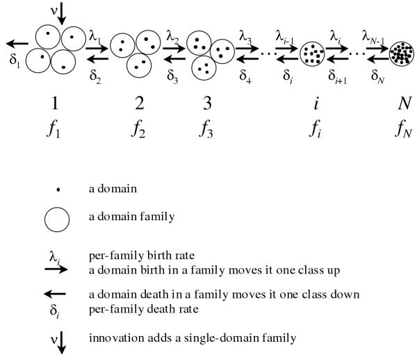
In a finite genome, the maximal number of domains in a family cannot exceed the total number of domains and, in reality, is probably much smaller; let N be the maximal possible number of domain family members. We consider classes of domain families, which have only one common feature, namely the number of members (Fig. 1). Let f_i be the number of domain families in i-th class, i.e. families that are represented by exactly i domains in the given genome, i = 1,2,...N. Birth of a domain in a family of class i results in the relocation of this family from class i to class i+1 (decrease of f_i and increase of f_i+1 by 1). Conversely, death of a domain in a family of class i relocates the family to class i-1; death of a domain in class 1 results in the elimination of the corresponding family from the given genome, this being the only considered mechanism of family death. We consider time to be continuous and suppose it very unlikely that more than one elementary event occur during a short time interval; formally, the probability that more than one event occurs during an interval Δt is o(Δt).

Figure 1.

Domain dynamics and elementary evolutionary events under BDIM.

The formulation of the model

The simple BDIM

Let us formulate the following independence assumption: i) all elementary events are independent of each other; ii) the rates of individual domain birth (λ) and death (δ) do not depend on i (number of domains in a family). Under this assumption, the instantaneous rate, at which a domain family leaves class i, is proportional to i and the following simple BDIM describes the evolution of such a system of domain family classes:

df₁(t)/dt = -(λ + δ) f₁(t) + 2δf₂(t) + ν

df_i(t)/dt = (i - 1)λf_i-1(t) - i(λ + δ)f_i(t) + (i + 1) δ f_i+1(t) for 1<i<N,     (2.1)

df_N(t)/dt = (N - 1)λ f_N-1(t) - Nδ f_N(t).

Similar models have been considered previously in several different contexts [33 v. 1, ch. 17, 34]. We will see in 3.2 that the solution of model (2.1) evolves to equilibrium, with a unique distribution of domain family sizes, f_i~(λ/δ)ⁱ/i; in particular, if λ = δ, then f_i~1/i. Thus, under the simple BDIM, if the birth rate equals the death rate, the abundance of a domain class is inversely proportional to the size of the families in this class. When the observations do not fit this particular asymptotic (as observed in several studies on distributions of protein family sizes), a different, more general model needs to be developed.

The Master BDIM

A more general BDIM emerges when the independence assumption is abandoned. Instead of constructing specific hypotheses regarding the dependence between the elementary events, let us simply suppose that the domain birth and death rates for a family of class i do not necessarily show proportionality to i. For the general case, we designate these rates, respectively, λ_i and δ_i; in the specific case of the simple BDIM (2.1), λ_i = λi and δ_i = δi. Then we have the following master BDIM:

df₁(t)/dt = -(λ₁ + δ₁)f₁(t) + δ₂f₂(t) + ν

df_i(t)/dt = λ_i-1f_i-1(t) - (λ_i + δ_i)f_i(t) + δ_i+1f_i+1(t) for 1<i<N,     (2.2)

df_N(t)/dt = λ_N-1f_N-1(t) - δ_Nf_N (t).

Let F(t)= f_i(t) be the total number of domain families at instant t; it follows from (2.2) that

dF(t)/dt = ν - δ₁f₁(t)     (2.3)

The system (2.2) has an equilibrium solution f₁,...f_N defined by the equality df_i(t)/dt = 0 for all i; this solution is described below under Proposition 1. Accordingly, there exists an equilibrium solution of equation (2.3), which we will designate F_eq (the total number of domain families at equilibrium). At equilibrium, ν = δ₁f₁, i.e. the processes of innovation and death of single domains (more precisely, the death of domain families of class 1, i.e. singletons) are balanced.

We can rewrite the model (2.2) in terms of the frequency of a domain family of class i p_i(t) = f_i(t)/F(t). Let x(t) = y(t)/Y(t); then

dx/dt = [dy/dt /y - dY/dt /Y] x.

Applying this identity to p_i(t) and rewriting equation (2.3) in the form

[dF(t)/dt]/F(t) = ν/F(t) - δ₁p₁(t)     (2.3')

we obtain the following model for frequencies of the domain family (master BDIM for frequencies), which is equivalent to (2.2):

dp₁(t)/dt = -(λ₁ + δ₁)p₁(t) + δ₂p₂(t) + ν/F(t) - (ν/F(t) - δ₁p₁(t))p₁(t),     (2.4)

dp_i(t)/dt = λ_i-1p_i-1(t) - (λ_i + δ_i)p_i(t) + δ_i+1p_i+1(t) - (ν/F(t) - δ₁p₁(t)) p_i(t) for 1<i<N,

dp_N(t)/dt = λ_N-1p_N-1(t) - δ_Np_N (t) - (ν/F(t) - δ₁p₁(t))] p_N(t).

System (2.4) should be solved together with equation (2.3).

The Master BDIM and Markov processes

Let us note that system (2.4) for frequencies is non-linear, so it is not a system of Kolmogorov equations for state probabilities of any homogeneous Markov process. Let us further suppose that a genome had ample time to arrive at an equilibrium with respect to the total number of domain families, such that F(t) = F_eq. This does not imply dp_i(t)/dt = 0 or df_i(t)/dt = 0; in other words, the system might rearrange the frequencies of individual families, although the total number of families remains stable. If F(t) = F_eq, the master system (2.4) turns into

d p₁(t)/dt = -(λ₁ + δ₁) p₁(t) + δ₂p₂(t) + ν/F_eq     (2.5)

d p_i(t)/dt = λ_i-1p_i-1(t) - (λ_i + δ_i) p_i(t) + δ_i+1p_i+1(t) for 1<i<N,

d p_N(t)/dt = λ_N-1p_N-1(t) - δ_Np_N (t).

System (2.5) can be rewritten as a matrix equation

dp(t)/dt = p(t)Q,

where p(t) = {p₁(t),...p_N(t)} and the matrix Q = (q_ij) is defined by equalities

q₁₁ = -(λ₁ + δ₁) + ν/F_eq, q₂₁ = δ₂ + ν/F_eq, q_s1 = ν/F_eq for all s > 2;

q_i-1,i = λ_i-1, q_i,i = -(λ_i + δ_i), q_i+1,i = δ_i+1, q_k,i = 0 for all k, |i-k| > 1, i = 2,...N-1,

q_N-1,N = λ_N-1, q_N,N = -δ_N.

It is easy to see that the sum of elements of each row (except for the first one) of the matrix Q is equal to ν/F_eq > 0. Therefore the matrix Q cannot be a matrix of transition rates for any Markov process (the sum of elements of each row of a matrix of transition rates for Markov process with continuous time should be non-positive [33 v. 1, ch.17, s. 8, 35 v. 2, ch. 3, s. 2]; in other words, there is no Markov process with continuous time and state space {1,2,...N} whose state probabilities satisfy system (2.5).

Thus, neither the initial BDIMs (2.1) or (2.2) nor the equilibrium model (2.5) can be described by any Markov process with continuous time.

Remark. If, in system (2.5), ν = 0, then this system turns into a system of state probabilities for a Markov birth and death process with continuous time.

Equilibrium in BDIMs

Equilibrium sizes and frequencies of the domain family system

Let us suppose that the genome had ample time to arrive at a complete equilibrium state, in which not only dF(t)/dt = 0, but also df_i(t)/dt = 0 for all i. Thus, the equilibrium sizes of domain families f_i satisfy the system

-(λ₁ + δ₁) f₁ + δ₂f₂ + ν = 0,

λ_i-1f_i-1 - (λ_i + δ_i)f_i + δ_i+1f_i+1 = 0 for 1<i<N,     (3.1)

λ_N-1f_N-1 - δ_Nf_N = 0.

It should be emphasized that the master model does not assign a priori the value of F_eq; this value has to be computed depending on the model parameters.

The following statement is central for further analysis.

Proposition 1. The master BDIM (2.2) has a unique equilibrium state (f₁,...f_N), which is the sole solution of system (3.1):

f₁ = ν/δ₁

f_i = ν λ_j / δ_j for all i = 2,...N.     (3.2)

The unique equilibrium state (3.2) is globally asymptotically stable.

In addition (formally assuming λ_j = 1 for i = 1),

F_eq = ν ( λ_j / δ_j     (3.3)

This proposition ascertains that all evolutionary trajectories of the system (2.2) exponentially (with respect to time) approach the equilibrium state (3.2). The proof is given in the Mathematical Appendix.

Remark. Let us denote the ratio of the birth rate to the innovation rate

G(N) ≡ λ_if_i/ν,

and the ratio of the death rate to the innovation rate

I(N) ≡ δ_if_i/ν.

Then, according to Proposition 1, for any BDIM in equilibrium,

G(N) - I(N) = λ_j / δ_j - λ_j/δ_j - 1 = -1.

The principal goal of the treatment that follows is the analysis of the asymptotic behavior of equilibrium frequencies and sizes of domain families (f₁,...f_N) at large N. We will differentiate two cases of asymptotic behavior according to the following

Definition. Let {q_i}, {s_i} be sequences of real numbers; let us denote q_is_i if lim q_i/s_i = 1 and q_i ~ s_i if lim q_i/s_i = c = const and 0<c<∞. We will also use this notation for finite but sufficiently long sequences.

Equilibrium frequencies for the simple BDIM

Let us apply Proposition 1 to the simple BDIM (2.1) with λ_i = λi, δ_i = δi.

Definition. A simple BDIM is balanced if θ = λ/δ = 1, i.e. if the rates of individual domain birth and death are equal.

Let us recall that a random discrete variable ξ has the logarithmic distribution with parameter θ < 1 if

P(ξ = i) = θⁱ/i [-ln(1-θ)]^-1, i = 1,2,...

A random variable ξ has the truncated logarithmic distribution with parameter θ if

P (ξ = i) = C_n θⁱ / i, i = 1,2,...n, C_n = 1/ θ^j/j.

Then, we have

Proposition 2.

1) For any simple BDIM (2.1)

f_i = (ν/δ)θ^i-1/i = (ν/λ)θⁱ/i,     (3.4)

F_eq = f_i = ν/δ θ^j-1/j,     (3.5)

and

p_i = (1/F_eq)(ν/δ)θ^i-1/i = (θⁱ/i) / θ^j/j     (3.6)

that is, the equilibrium frequencies have the truncated logarithmic distribution if θ < 1.

2) If a simple BDIM is balanced, then

F_eq = ν/δ 1/j,     (3.7)

and for all i = 1,2,...N

p_i = ν/δF_eq/i = ( 1/j)^-1 / i.     (3.8)

The proof is given in the Mathematical Appendix.

Thus, a simple BDIM can have equilibrium frequencies only of the form p_i = Cθⁱ/i, where C = const and θ is the distribution parameter. In particular, the equilibrium frequencies for a balanced simple BDIM have the power distribution with the degree equal to -1.

Simple methods exist for preliminary graphical estimation of the single distribution parameter θ [36 ch. 7, s. 7]. We will prove in the following section that, if we observe a power asymptotic for empirically observed equilibrium frequencies, then (assuming that the system can be described by a BDIM), the rates λ_i and δ_i should be asymptotically equal at large i. If, additionally, the degree of the asymptotic is not equal to -1, then the system dynamics cannot be described by a simple BDIM. In this case, it is necessary to consider more general models, such as the Master BDIM (2.2).

Asymptotic behavior of equilibrium frequencies of a Master BDIM: Main Theorems

Let us consider the master BDIM (2.2); we showed in 3.1 that its equilibrium frequencies are the solution of the system

-(λ₁ + δ₁)p₁ + δ₂p₂ + ν/F_eq = 0,     (3.9)

λ_i-1p_i-1 - (λ_i + δ_i)p_i + δ_i+1p_i+1 = 0 for 1<i<N,

λ_N-1p_N-1 - δ_Np_N = 0.

The following theorem gives all possible types of asymptotic behavior of the equilibrium frequencies and defines the connections between these asymptotics depending on model parameters. In particular, if there is no information on the exact form of dependence of the rates of birth and death of domains on the size of a domain family, the theorem can be used to qualitatively describe the dynamics of the asymptotic behavior of the equilibrium frequencies.

We will prove that the asymptotic behavior of a solution of system (3.9) is completely defined by the asymptotic relation between λ_i and δ_i. More precisely, let us define a function χ (i)= λ_i-1/δ_i; we consider only functions of power growth, i.e. χ (i) ~ i^s at i→∞ for a real s. We will see that this is not a serious restriction because the most realistic situations correspond to the case of s = 0. So, let us suppose that, for large i, the following expansion is valid:

χ (i) ≡ λ_i-1/δ_i = i^s θ (1+a/i + O(1/i²))     (3.10)

where s, a are real numbers and θ > 0. Evidently, if s ≠ 0, χ (i) tends either to 0 (s < 0) or to ∞ (s > 0) with the increase of i.

Definition. Let us refer to a BDIM (2.2), (3.10) as

i. non-balanced, if s ≠ 0;

ii. first-order balanced, if s = 0 and θ ≠ 1, i.e.

λ_i-1/δ_i = θ (1+a/i + O(1/i²)) at large i;     (3.11)

iii. second-order balanced, if s = 0, θ = 1 and a ≠ 0, i.e.

λ_i-1/δ_i = 1 + a/i + O(1/i²)) for large i;     (3.12)

iv. high-order balanced, if s = 0, θ = 1 and a = 0, i.e.

λ_i-1/δ_i = 1 + O(1/i²)) for large i.

We will show that the first three coefficients, s, θ and a, of asymptotic expansion (3.10) for χ (i) = λ_i-1/δ_I exactly specify all possible asymptotic behaviors of BDIM equilibrium frequencies.

Theorem 1. The equilibrium frequencies p_i of BDIM (2.2) have the following asymptotics

i. if the model is non-balanced, then

p_i ~ Γ (i)^sθⁱi^a, where Γ (i) is the Γ-function;

ii. if the model is first-order balanced, then

p_i ~ θⁱi^a;

iii. if the model is second-order balanced, then

p_i ~ i^a;

iv. if the model is high-order balanced, then

p_i ~ 1

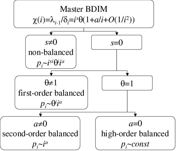
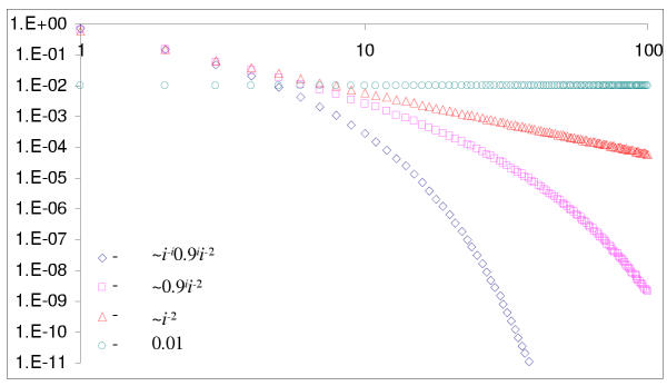
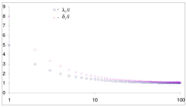
The proof is given in the Mathematical Appendix. The classification of BDIM according to the order of balance is illustrated in Fig. 2 and the asymptotics for different types of BDIMs are shown in Fig. 3.

Figure 2.

Different orders of balance in BDIMs.

Figure 3.

Asymptotics of equilibrium distributions for balanced BDIMs of different orders.

It follows from this theorem that, if a BDIM is non-balanced, then its equilibrium frequencies p_i (and equilibrium family sizes f_i) increase or decrease extremely fast (hyper-exponentially) with the increase of i. In contrast, if a BDIM has a non-zero order of balance, asymptotic behavior is observed.

Let us recall that a random discrete variable ξ has the Pascal (or negative binomial) distribution with parameters (r,q), r > 0, 0 <q < 1, if P(ξ = k) = Γ(r+k)/[Γ(r) Γ(1+k)] (1-q)^rq^k[36]. We will say that sequence {p_i} follows (or asymptotically has) a discrete probabilistic distribution {q_i} if p_i ~ q_i for large enough i.

Corollary 1.For a first-order balanced BDIM with θ < 1,

i. if a > -1, the equilibrium frequencies p_i follow Pascal distribution with parameters (a+1,θ);

ii. if a = -1, the equilibrium frequencies follow truncated logarithmic distribution with parameter θ;

iii. if a = 0, the equilibrium frequencies follow geometric distribution with parameter θ.

The following implication of Theorem 1 is of principal interest.

Corollary 2. Equilibrium frequencies of a BDIM have a power asymptotic behavior if and only if the BDIM is second-order balanced.

Corollary 3. For high-order balanced BDIM, if λ_i-1/δ_i = 1 for all i, the only possible distribution of equilibrium frequencies is uniform, p_i = const for all i. Moreover, even if λ_i-1/δ_i = 1 + O(1/i²), the equilibrium frequencies asymptotically tend to the uniform distribution.

Rational BDIM

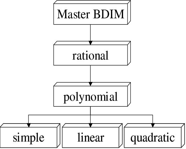
Rational models comprise a general class of BDIM (Fig. 4), for which the asymptotic behavior of the equilibrium frequencies and equilibrium sizes of domain families can be completely investigated.

Figure 4.

The hierarchy of BDIM types.

Let us suppose that the birth and death rates are of the form

λ_i = λ P(i) = λ (i + a_k)^α_k,     (4.1)

δ_i = δ Q(i) = δ (i + b_k)^β_k

for i > 0, where λ, δ are positive constants, α_k, β_k are real and a_k, b_k are non-negative for all k = 1,...N.

We will refer to BDIM (2.2.), (4.1) as rational BDIM.

It is known that a wide class of mathematical functions can be well approximated by rational functions of the form (4.1) (see, e.g. [37]).

Specific cases of the rational BDIM are simple BDIM with P(i) = i, Q(i) = i, linear BDIM with P(i) = i + a₁, Q(i) = i + b₁, where a₁, b₁ are constants, and polynomial BDIM, if P(i) and Q(i) are polynomials on i.

The following theorem describes all possible asymptotic behaviors of the equilibrium frequencies of a rational BDIM. Let us denote

θ =λ/δ,

η = α_k - β_k,

ρ = a_kα_k - b_kβ_k,

β = β_k.

Theorem 2. The equilibrium sizes of domain families of a rational BDIM have the following asymptotics

f_iCν/λ Γ(i)^η θⁱi^ρ-β     (4.2)

where the constant C = (Γ(1 + b_k)^β_k/ Γ(1 + a_k)^α_k.     (4.3)

The proof is given in the Mathematical Appendix.

Corollary 1. If η = 0, then the rational BDIM is first-order balanced and the sequence of equilibrium numbers of domain families {f_i} has a power-exponential asymptotics

f_iCν/λ θⁱi^ρ-β.     (4.4)

In particular, if ρ - β > -1, the equilibrium frequencies p_i follow the Pascal distribution with parameters (ρ - β + 1, θ);

if ρ - β = -1, then frequencies p_i follow the truncated logarithmic distribution;

if ρ - β = 0, then frequencies p_i follow the geometric distribution.

Corollary 2. The equilibrium sizes of domain families f_i and equilibrium frequencies p_i for a rational BMID have the power asymptotics if and only if η = 0 and λ = δ, i.e. the BDIM is second-order balanced, in which case

f_iCν/λ i^ρ-β.     (4.5)

Formula (4.4) gives the asymptotics for the equilibrium sizes of domain families f_i and, accordingly, for the total number of families F_eq. The exact expressions for these quantities are given in the proofs of Theorem 2 and Lemma (see Mathematical Appendix).

Proposition 3.

i. The equilibrium sizes of domain families f_i of a balanced (first or higher order) rational BDIM are

f_i = Cν/δθ^i-1 [(Γ(i + a_k))^α_k]/ [(Γ(i + 1 + b_k))^β_k] for all i = 1,2,...

where

C = [(Γ(1 + b_k))^β_k]/ (Γ(1 + a_k)^α_k].

ii. The total number of domain families at equilibrium is

F_eq = Cν/δ( θ^j-1 (Γ(j + a_k))^α_k/ (Γ(j + 1 + b_k))^β_k).

For the rational, second-order balanced BDIM, the ratio of the birth rate to the innovation rate is

G(N) = θⁱ [Γ(i + 1 + a_k)/Γ(1 + a_k)]^α_k / [Γ(i + 1 + b_k) / Γ(1 + b_k)]^β_k.

The asymptotic formulas for equilibrium frequencies of rational BDIM could be considered as particular cases of the corresponding formulas of general theorem 1. Proposition 3 allows one to calculate the constants in the corresponding asymptotic formulas for the sizes of domain families for a rational BDIM. If only equilibrium frequencies are analyzed, the values of these constants become irrelevant because they contract. However, if the actual values of f_i and F_eq are of interest, the values of the constants are required.

Properties of the main types of rational BDIM

Simple BDIM

As shown above, a simple BDIM can have equilibrium frequencies only of the form p_i = Cθⁱ/i, C = const;in particular, if the distribution parameter θ < 1, we get the (truncated) logarithmic distribution. Logarithmic distributions are seen in many biological contexts, e.g., the distribution of species by the number of individuals in populations or, what is more relevant, the distribution of protein folds by the number of families per fold [38]. Thus, a simple BDIM could be potentially used for modeling the dynamics of biological systems with a logarithmic distribution of equilibrium densities. We examine this possibility in greater detail starting with the case λ = δ (second-order balanced simple BDIM).

We can extract from Proposition 2 some additional information, which could be helpful for estimating the model parameters. It is known that

1/i = lnN + C_E + O (1/N), where C_E is the Euler constant, C_E = 0.5772157...

More precisely, the approximation 1/i = lnN + C_E + N^-1/2 - N^-2/12 has an error less then 10^-6 for N > 10. Thus, from (3.7), we obtain an interesting formula

F_eq (ν/δ) [lnN + C_E]     (5.1)

This means that, in the equilibrium state of the system, the total number of domain families grows only slowly (~ln N) with the increase of the maximal number (N) of domains in a family (which is equal to the maximal possible number of domain family size classes).

Furthermore, according to equation (2.3), in the equilibrium state of a simple BDIM ν/δ = f₁, so we have

F_eq / f₁ lnN + C_E     (5.2)

Formula (5.1) can be used for estimating the model parameters on the basis of empirical data.

In the more general case λ ≠ δ, we can also obtain an estimate of the rate of innovation ν. If λ < δ (θ < 1), then the series in the right part of (3.5) quickly converges,

θ^i-1/i → -ln(1-θ)/θ,

so -ln(1-θ)/θ is a good approximation for the sum θ^i-1/i for large N. Then

F_eq = (ν/δ) θ^i-1/i = (ν/λ) θⁱ/i ν/λ (-ln(1-θ)),

and

ν/δ = F_eq θ/(-ln(1-θ)).     (5.3)

Taking into account that ν/δ = f₁ (2.3), we have a relation

F_eq/f₁ -ln(1-θ)/θ,     (5.4)

which allows the parameter θ to be estimated on the basis of empirical data.

If N can be estimated independently and is not very large, we can use more exact relations:

θⁱ/i -ln(1-θ) + Ei(-N(1-θ)) - N^-1/2 + N^-2/12.

where the function .

Further, if (1-θ)N is small (i.e., θ is very close to 1), then the approximation

θⁱ/iC_E - N(1-θ)

has an error less then [N(1-θ)]²/4 and, in this case,

F_eq/f₁ (C_E - N(1 - θ))/θ.     (5.5)

If (1 - θ)N is large, then the following inequalities provide simple bounds for F_eq/f₁ = θ^i-1/i:

-(ln(1-θ)/θ-θ^N/[(N+1)(1-θ)] < θ^i-1/i < -ln(1-θ)/θ-θ^N[1/(N+1)-θ/(N+2)].     (5.6)

For the simple BDIM, the ratio of the rate of duplications to the innovation rate is

G(N) = λ_if_i/ν = θⁱ = θ(1-θ^N-1)/(1-θ),

so G(N) → ∞ if θ > 1 and G(N) → 1/(1-θ) if θ < 1 at N→∞.

If the simple BDIM is the 2^nd order balanced, θ = 1, then G(N) = N - 1.

Thus, for the simple, second-order balanced BDIM, the number of duplications per time unit is N-1 times greater than the number of innovations.

The total number of domains in the equilibrium state for the simple BDIM is

M(N) = if_i = ν/λθ(1-θ^N)/(1-θ).

If a simple BDIM is second-order balanced, then G(N) = ν/λ N.

Linear BDIM

We saw that the assumption of independence of birth and death rates of individual domains on each other and on the size of domain families is incompatible with any power distribution of the equilibrium frequencies with the degree not equal to -1. The simplest case of a BDIM, which can have, depending on the parameters, three types of asymptotic behavior described by Theorem 1 (excluding the first one, hyper-exponential, which corresponds to a non-balanced BDIM; all linear BDIMs are balanced) and, in particular, any power asymptotics, is a model with linear birth and death rates of the form:

λ_i = λ (i + a), δ_i = δ (i + b), where a and b are constants.     (5.7)

The parameters a and b account, in the simplest possible form, for the deviation of the domain birth and death rates from those under the independence assumption. More precisely, according to (5.7), the average birth rate per domain in a family of size i is λ_i/i = λ + λa/i. So, for small i, the average birth rate is close to λ + λa, whereas, for large i, it tends to λ. Similarly, the average death rate changes from δ + δb in a small family to the limit value δ in a large family. Thus, if a and b are positive (which seems to be the case for the available data; see below), both the birth rate and the death rate per domain decrease with the increase of the class number (size of the respective domain families); conversely, if a and b are negative, these rates increase with the class number (Fig. 5).

Figure 5.

Dependence of per domain birth and death rates on the domain family size for the second-order balanced linear BDIM.

Corollary 1 of Theorem 2 implies that equilibrium frequencies p_i of a linear BDIM have asymptotics

p_i ~ θⁱi^a-b-1, where θ = λ/δ.     (5.8)

In particular, if λ ≠ δ and a = b, the linear BDIM is first-order balanced and the equilibrium frequencies p_i follow the logarithmic distribution (in this case, the linear BDIM is asymptotically equivalent to the simple BDIM). If λ = δ, the linear BDIM is second-order balanced and the equilibrium frequencies p_i follow the power distribution

p_i ~ i^a-b-1.     (5.9)

Thus, the dependence of the domain frequency on the family size is actually determined by the difference a - b. If a >b, the birth rate decreases faster than the death rate with the increase of family size, i. e. there seems to be a "competition" between domains in a family; in contrast, if a <b, the death rate drops faster, i.e. a "synergy" between domains appears to exist (Fig. 4).

More detailed information can be obtained using Proposition 4:

i) for a first-order balanced linear BDIM, the equilibrium sizes f_i of domain families are

f_i = cν/δθ^i-1Γ(i + a)/(Γ(i + 1 + b)) for all i

where

c = Γ (1 + b)/Γ (1 + a)

and the total number of domain families at equilibrium is

F_eq = cν/δ[ θ^j-1Γ(j + a) / (Γ(j + 1 + b)].     (5.10)

ii) for a second-order balanced linear BDIM (θ = 1),

f_i = c₁ν/δ Γ (i + a)/Γ (i + 1 + b)

and

According to (2.3), in the equilibrium state of a linear BDIM, f₁ = ν/δ₁ = ν/(δ(1 + b)) and so, for a second-order balanced linear BDIM, we have the formula

Suppose that equilibrium frequencies obtained from empirical data follow the power distribution p_i ~ i^-γ; in this case, -γ is the slope of the empirical curve (lnf_i versus lni) and can be estimated from the data. Assuming that the system is well described by a linear BDIM, it follows from (5.9) that a - b = 1 - γ and λ = δ. Thus,

f_i = cν/δ Γ (i + a)/Γ (i + a + γ), where c = Γ (γ + a)/Γ (1 + a),     (5.12)

and

where a is the single free parameter.

For the linear second-order balanced BDIM, the ratio of the birth rate to the innovation rate is

if 1 + a - b ≠ 0. As

if 1 + a - b < 0 and G(N)→∞ if 1 + a - b > 0 at N→∞.

The case 1 + a - b = 0 (slope of the asymptote in double logarithmic coordinates equal to a - b - 1 = -2) is a critical one.

In this case,

G(N) = Γ(1 + b) / Γ(b) Γ (i + b) / (Γ (i + 1 + b) =

b₁/(i + b) = b [PolyGamma(0, b+N) - PolyGamma(0, b+1)].

Accordingly, G(N)→∞ at N→∞.

The total number of domains in the equilibrium state for a second-order balanced linear BDIM is

If the slope of the asymptote γ = -1, the linear second-ordered BDIM shows the same asymptotic behavior as a simple BDIM (2.1), but behaves differently at small i. If γ ≠ -1, the system cannot be described by a simple BDIM even asymptotically, but can be described by a linear BDIM. As indicated above, in this case, the average per-domain birth and death rates depend on the size of the domain family and the difference a-b characterizes this dependence.

Quadratic BDIM

The linear BDIM takes into account the dependence of average birth and death rates of individual domains on the size of domain family, but does not imply a specific form of interaction between domains. Let us consider the simplest, pairwise interaction, which leads to λ_i ~ i² and/or δ_i ~ i², i.e. one or both rates are polynomials on i of the second degree. If these degrees are different (i.e., λ_i ~ i and δ_i ~ i²), then the corresponding BDIM is non-balanced and equilibrium frequencies have hyper-exponential asymptotics. Thus, let

λ_i = λ (i² + r₁i + r₂), δ_i = δ (i² + q₁i + q₂),     (5.13)

where r_k, q_k, k = 1,2 are constants (such that λ_i, δ_i are positive for all i) or

λ_i = λ (i + a₁)(i + a₂),

δ_i = δ (i + b₁)(i + b₂)

Then, r₁ = a₁ + a₂, q₁ = b₁ + b₂, and

χ (i) = λ_i-1/δ_i = θ (1 + (r₁-q₁-2)/i + O(1/i²)),

where θ = λ/δ.

According to theorem 3 and Proposition 3, the quadratic BDIM with rates (5.13) has equilibrium sizes of domain families

f_i = c₂ ν/δ θ^i-1 Γ (i + a₁) Γ (i + a₂) / (Γ (i + 1 + b₁) (Γ (i + 1 + b₂)) c₂ν/δ θ^i-1i^ρ-2     (5.14)

where ρ = r₁ - q₁ and the constant c₂ = [(Γ (1+b₁) Γ (1+b₂)] / [Γ (1+a₁) Γ (1+a₂)], and the total number of domain families at equilibrium

F_eq = c₂ν/δ ( θ^j-1 Γ(j+a₁) Γ(j+a₂) / (Γ(j+1+b₁) (Γ(j+1+b₂)).     (5.15)

Note that the asymptotic behavior of frequencies p_i does not depend on free coefficients r₂, q₂ in (5.13), but only on θ and r₁-q₁ (as follows from (5.14)), although the values of f_i are proportional to the constant c₂, which could depend on the free coefficients r₂, q₂. Let us consider the case r₂ = q₂ = 0 in more detail.

If only square terms are present in the expressions for the birth and death rates, λ_i = λi², δ_i = δi², then a_k = b_k = 0, k = 1,2 and so c₂ = 1, f_i = ν/δ θ^i-1/i² and F_eq = ν/δ θ^j-1/j². So at N→∞

F_eq ν/δ θ^j-1 / j² = ν/λ Polylog(2,θ)     (5.16)

where Polylog is a special function, Polylog(k,x) = x^j/j^k.

According to (3.2), f₁ = ν/δ₁; for this particular case of quadratic BDIM, f₁ = ν/δ and

F_eq/f₁ Polylog(2,θ).     (5.17)

Formula (5.17) allows estimating parameter θ from empirical data if N is large enough.

More precisely, F_eq = ν/λ θ^j/j² = ν/λ (Polylog(2,θ)-θ^1+N LerchPhi(θ,2,1+N)), where LerchPhi is a special function (these and other special functions used below can be computed using program packages Mathematika or Maple).

If, additionally, θ = 1 (the BDIM is second-order balanced), then

f_i = (ν/δ)/i² = f₁/i²     (5.18)

and, at large N

F_eq ν/δ π²/6 1.645 ν/δ = 1.645f₁.     (5.19)

From formulas (5.8), (5.15), we can extract some additional information, which could be helpful for estimating the model parameters at relatively small N. Let us recall definitions of some special functions.

The digamma function φ(z) is logarithmic derivative of Γ(z), φ(z) = Γ'(z)/Γ(z).

The function PolyGamma(n,z) is n^th derivative of φ(z), PolyGamma(n,z) = dⁿφ(z)/dzⁿ, such that φ(z)= PolyGamma(0,z).

It is known that

1/i² = π²/6-PolyGamma(1,1+N),

Thus we have

F_eq = ν/δ 1/j² = ν/δ [π²/6-PolyGamma(1,1+N)]     (5.20)

F_eq/f₁ = π²/6-PolyGamma(1,1+N),

which can be used for estimating unknown parameters of the model.

The values of PolyGamma(1,x) are tabulated and can be computed using standard program packages; for a rough preliminary estimate, PolyGamma(1,x) = 1/x+1/2x²+O(1/x⁴).

If linear terms are also present in the quadratic BDIM, λ_i = λ (i²+a₁i), δ_i = δ (i²+b₁i), then

f_i = c₂ν/δ θ^i-1/i Γ (i+a₁)/Γ (i+1+b₁)

where c₂ = Γ (1+b₁)/Γ (1+a₁); F_eq = Σf_i can be computed using special functions. In particular, if the BDIM is second-order balanced, θ = 1, then

f_i = c₂ν/δ Γ (i+a₁) / (i Γ (i+1+b₁)).

For this variant of the model, f₁ = ν/δ₁ = ν/(δ(1+b₁)), and so

Polynomial BDIMs

The quadratic models take into account the dependence of birth and death rates of individual domains on the simplest, pairwise interactions. If interactions of higher orders are postulated, λ_i ~ P_n(i) and/or δ_i ~ Q_m(i), where P_n(i), Q_m(i) are polynomials on i of the n-th and m-th degrees. Again, if the degrees n and m are different, then the BDIM is non-balanced and equilibrium frequencies have hyper-exponential asymptotics. Thus, let n = m,

λ_i = λR (i) = λ r_ki^m-k, δ_i = δQ(i) = δ q_ki^m-k     (5.21)

where r_k, q_k are constants and r₀ = q₀ = 1. We suppose, of course, that R(i), Q(i) are positive for all integer i. Note that, in this case, χ (i) ≡ λ_i-1/δ_i = θ (1+(r₁ - q₁ - m)/i+O(1/i²)), where θ = λ/δ. We will suppose that θ ≤ 1.

According to Theorem 3, the polynomial BDIM with rates (5.21) has equilibrium sizes of domain families with power-exponential asymptotics

f_i ~ θⁱi^ρ-m     (5.22)

where ρ = r₁ - q₁.

In particular, if ρ - m > -1, the equilibrium frequencies p_i follow the Pascal distribution with parameters (ρ - m + 1, θ);

if ρ - m = -1, the equilibrium frequencies p_i follow the (truncated) logarithmic distribution;

if ρ - m = 0, the equilibrium frequencies p_i follow the geometric distribution;

if λ = δ, the polynomial BDIM is second-order balanced and the equilibrium frequencies p_i follow the power distribution

p_i ~ i^ρ-m.     (5.23)

Note that the degree of the power distribution (5.23) depends only on m, the common degree of the polynomials (5.21), and on ρ, the difference between the coefficients r₁ and q₁, and does not depend on other coefficients. In particular, if r₁ = q₁, then p_i ~ i^-m. This relation could be interpreted as follows: if the first two coefficients of polynomial rates λ_i and δ_i are equal, then the degree of the power distribution (5.19) is equal to the "order of interactions" of domains.

Formula (5.22) can be refined. Let R(i) = (i+a_k), Q(i) = (i+b_k).

Then (see Proposition 3) the equilibrium numbers of domain families f_i of the polynomial BDIM (5.18) are

f_i = Cν/δθ^i-1 [Γ(i+a_k)/Γ(i+1+b_k)]

where C = [Γ(1+b_k)/Γ(1+a_k)], and the equilibrium total number of domain families

F_eq = Cν/δ θ^j-1 [Γ(j+a_k)/Γ(j+1+b_k)].

For the polynomial model f₁ = ν/δ₁ = ν/(δ q_k), so

F_eq/f₁ = C θ^j-1 (Γ(j+a_k)/Γ(j+1+b_k))/q_k.

This formula can be used for estimating the model parameters.

For the polynomial second-order balanced BDIM, the ratio of the death rate to the innovation rate is

G(N) = λ_if_i/ν = ( Γ(1+b_k)/Γ(1+a_k)) Γ(i+1+a_k)/Γ(i+1+b_k) =

[Γ(i+1+a_k)/Γ(1+a_k)]/[Γ(i+1+b_k)/Γ(1+b_k)].

Approximation of the observed domain family size distributions in prokaryotic and eukaryotic genomes with different BDIMs

Having developed the mathematical theory of BDIMs, we sought to determine which of these models, if any, adequately described the empirical data on domain family size distribution. To identify the domain sets of domains encoded in each of the genomes, the CDD library of position-specific scoring matrices (PSSMs), which includes the domains from the Pfam and SMART databases, was used in RPS-BLAST searches [12] against the protein sequences from a set of completely sequenced eukaryotic and prokaryotic genomes http://www.ncbi.nlm.nih.gov/entrez/query.fcgi?db=Genome. The CDD domain library is partially redundant, so when the results obtained from individual PSSMs showed significant overlap (more than 50% of hits overlapped for more than 50% of their length), the corresponding domains were examined case-by-case for redundancy. PSSMs representing structurally similar domains and producing overlapping lists of hits were joined into "synonymy clusters".

The results of RPS-BLAST searches against the sets of protein sequences from individual genomes were interpreted as follows: non-overlapping hits to the same protein were treated independently; among overlapping hits, only the strongest one (lowest E-value) was recorded; all hits from a synonymy cluster were assigned to one representative domain family. The number of hits that a domain family had in a genome, with the cut-off of E = 0.001, was recorded as the number of domains of the given family encoded in the given genome. The CDD domain library certainly does not include all existing domains. In practice, domains from this collection were detected in >50% in each of the analyzed species, with the only exception of human, for which the analyzed protein set is likely to contain a substantial fraction of false predictions (Table 1).

Table 1.

Domain families in sequenced genomes and parameters of the best-fit second-order balanced linear BDIM

	No. of ORFs in genome	No. of detected domain families	No. of detected domains	No. of ORFs with RPS-BLAST hits	Maximum size of a family	f1 (f'1)	a	b	k	ν/δ = ν/λ	G = λifi/ν
Sceb	6340	1080	4575	3331	130	420 (436)	1.55	3.27	-2.72	1861.8	[3.28..3.53]
Dme	13605	1405	11734	7262	335	426 (435)	1.62	2.79	-2.17	1648.2	[8.44..15.50]
Cel	20524	1418	17054	11090	662	423 (421)	1.13	2.03	-1.89	1273.0	[16.18..∞ ]
Ath	25854	1405	21238	15006	1535	270 (277)	3.80	4.98	-2.18	1657.7	[17.09..26.89]
Hsa	39883	1681	27844	16755	1151	298 (288)	5.16	6.43	-2.27	2136.2	[17.14..22.88]
Tma	1846	772	1683	1268	97	501 (499)	0.14	2.22	-3.08	1606.4	[1.04..1.06]
Mth	1869	693	1480	1150	43	438 (436)	0.12	2.00	-2.88	1305.3	[1.18..1.27]
Sso	2977	695	1950	1614	81	386 (385)	0.36	2.04	-2.68	1167.8	[1.83..2.00]
Bsu	4100	1002	3413	2502	124	507 (510)	0.48	2.01	-2.53	1534.6	[2.46..2.79]
Eco	4289	1078	3624	2765	140	523 (519)	0.84	2.54	-2.70	1837.0	[2.45..2.61]

a: f₁(f'₁), the observed (predicted) number of domains in class 1 (represented only once in the genome); a, b, parameters of the second-order balanced linear BDIM; k, slope of the power asymptotic; ν/δ = ν/λ, ratio of the innovation rate to the per domain death (birth) rate; G, ratio of the innovation rate to the total (per genome) birth rate. b: Species abbreviations: Sce, Saccharomyces cerevisiae, Dme, Drosophila melanogaster, Cel, Caenorhabditis elegans, Ath, Arabidopsis thaliana, Hsa, Homo sapiens, Tma, Thermotoga maritima, Mth, Methanothermobacter thermoautotrophicum, Sso, Sulfolobus solfataricus, Bsu, Bacillus subtilis, Eco, Escherichia coli.

To enable statistical analysis using the χ²-method for the entire range of the data, including the sparsely distributed classes corresponding to large families, the data needed to be combined. For each genome, the observed domain family frequencies were grouped into bins, each containing at least 10 families; typically, bins corresponding to families with small number of members included a single size class (e.g. all single-member families, two-member families etc), whereas bins corresponding to large families may span hundreds of size classes, most of them empty. Theoretical distribution values for a bin combining observed data from m-th to n-th class were computed as , where f'_i is the predicted number of families in the i-th class and depends on the model parameters. Since the model displays only a weak dependence on the maximum number of domains in a family (N), instead of including N as a model parameter, the sum (where i_max is the number of domains in the most abundant of the detected families), was normalized to equal the total number of families detected in the given genome (a requirement for the χ² analysis). χ² values were computed to measure the quality of fit between the observed and the theoretical distributions. The distribution parameters (θ for the simple BDIM, a and b for the second-order balanced linear BDIM) were adjusted to minimize the χ² value.

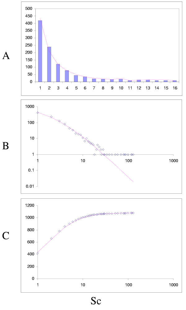
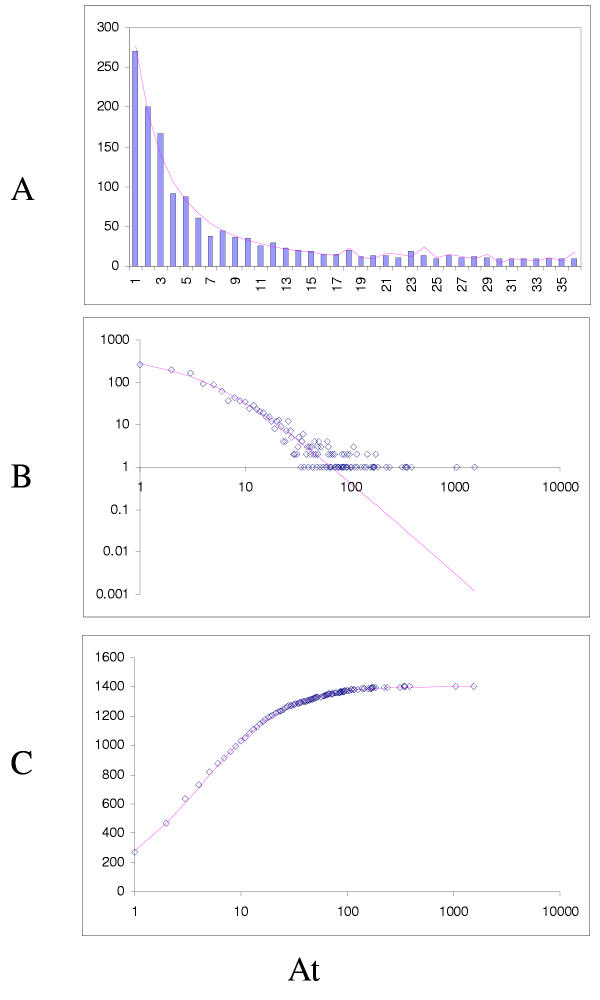
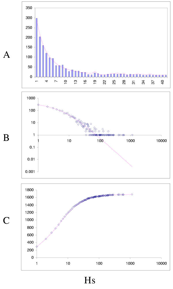
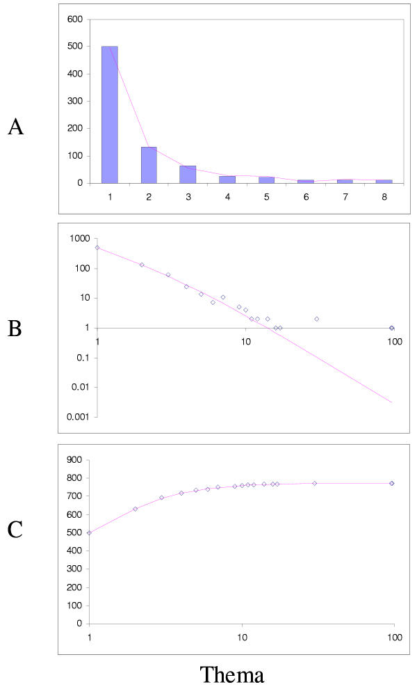
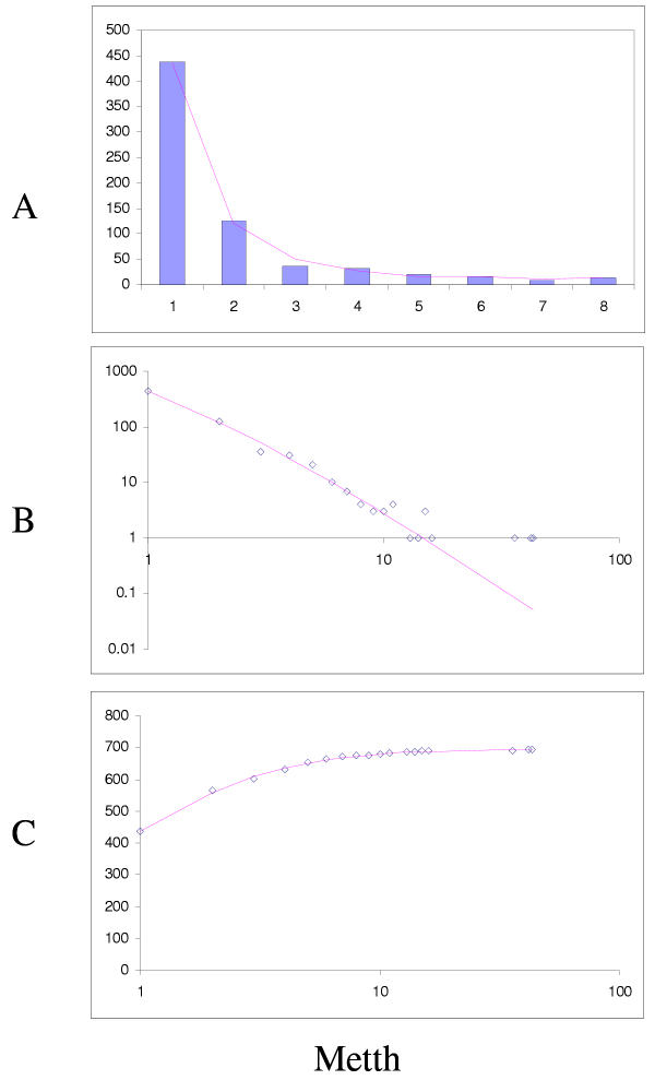
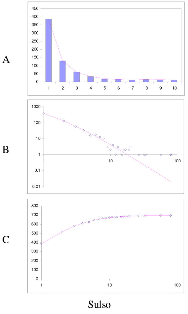
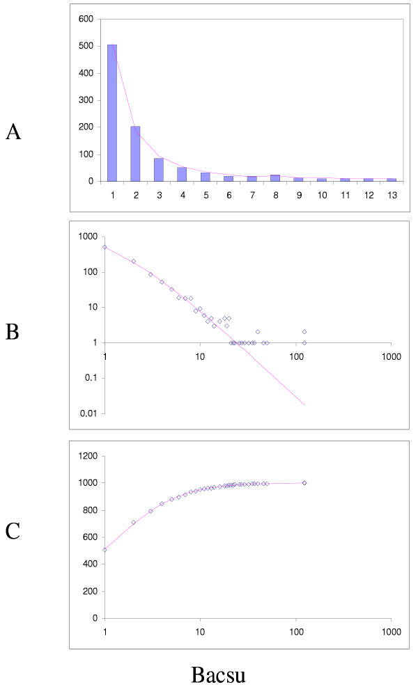
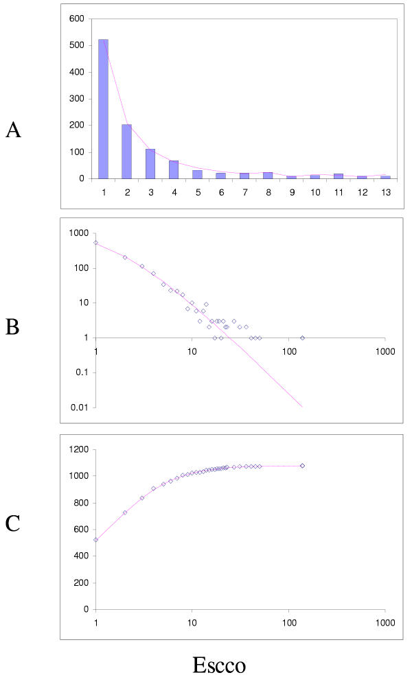
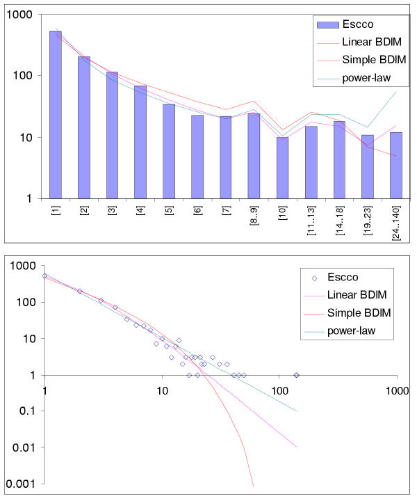
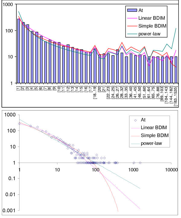
The simplest model that resulted in a good fit to the observed domain family size distributions was the second-order balanced linear BDIM (Fig. 6,7,8,9,10,11,12,13,14,15). For all analyzed genomes, P(χ²) for this model was >0.05, i.e. no significant difference between the model predictions and the observed data was detected. Considering the first-order balanced linear BDIM, which involves varying the parameter θ, did not result in a significant improvement of fit for any of the analyzed genomes (data not shown). In contrast, a fit to a truncated logarithmic distribution (prediction of a simple BDIM) failed for all genomes (P(χ²) < 10^-5; Fig. 16, 17, and data not shown). An exact power-law distribution, which is often used to approximate protein family frequency distributions, similarly failed to adequately fit the observed data, even when the most deviant class 1 families were excluded (P(χ²) = 0.0013 for T. maritima; P(χ²) < 10^-5 for the rest of the genomes; Fig. 16, 17 and data not shown). Notably, second-order balanced linear BDIM results in a correct prediction of the number of very large families, whereas simple BDIM systematically underestimates the number of families in the highest bins. Conversely, the power-law fit underestimates the slope of the best-fit line (in double logarithmic coordinates) compared to the asymptote of the linear BDIM prediction and, accordingly, significantly overestimates the number of families in the highest bins (Fig. 16, 17). These results are compatible with the recent observation that the domain family size distributions are better described by the generalized Pareto distribution than by power laws [31].

Figure 6.

Fit of empirical domain family size distributions to the second-order balanced linear BDIM: the yeast Saccharomyces cerevisiae. A. Distribution of the size of domain families grouped into bins B. Domain family size distribution in double logarithmic coordinates. Magenta line: f_i = 11521Γ(i+1.55)/Γ(i+4.27) C. Cumulative distribution function of domain family size. The line shows the prediction of the second-order balanced linear BDIM.

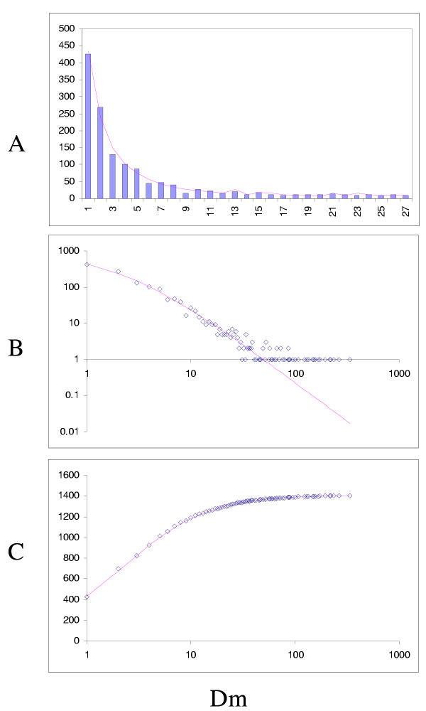
Figure 7.

Fit of empirical domain family size distributions to the second-order balanced linear BDIM: the fruit fly Drosophila melanogaster. The panels and the designations are as in Fig. 6. B. Magenta line: f_i = 5258Γ(i+1.62)/Γ(i+3.79)

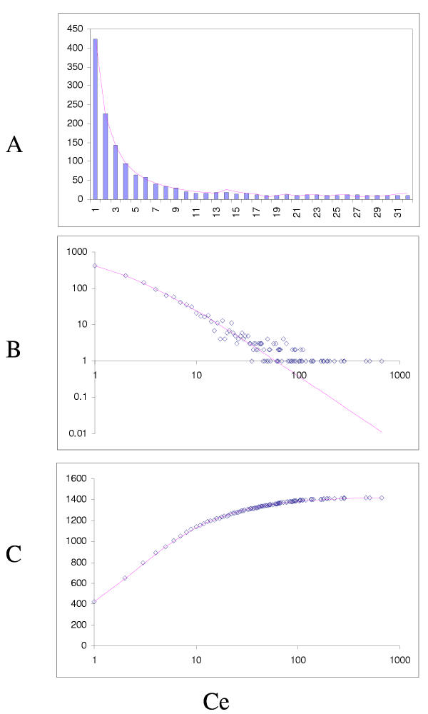
Figure 8.

Fit of empirical domain family size distributions to the second-order balanced linear BDIM: the nematode worm Caenorhabditis elegans. The panels and the designations are as in Fig. 6. B. Magenta line: f_i = 2453Γ(i+1.13)/Γ(i+3.03)

Figure 9.

Fit of empirical domain family size distributions to the second-order balanced linear BDIM: the thale cress Arabidopsis thaliana. The panels and the designations are as in Fig. 6. B. Magenta line: f_i = 10750Γ(i+3.80)/Γ(i+5.98)

Figure 10.

Fit of empirical domain family size distributions to the second-order balanced linear BDIM: Homo sapiens. The panels and the designations are as in Fig. 6. B. Magenta line: f_i = 22030Γ(i+5.16)/Γ(i+7.43)

Figure 11.

Fit of empirical domain family size distributions to the second-order balanced linear BDIM: the hyperthermophilic bacterium Thermotoga maritima. The panels and the designations are as in Fig. 6. B. Magenta line: f_i = 4256Γ(i+0.14)/Γ(i+3.22)

Figure 12.

Fit of empirical domain family size distributions to the second-order balanced linear BDIM: the thermophilic euryarchaeon Methanothermobacter thermautotrophicus. The panels and the designations are as in Fig. 6. B. Magenta line: f_i = 2753Γ(i+0.12)/Γ(i+3.00)

Figure 13.

Fit of empirical domain family size distributions to the second-order balanced linear BDIM: the hyperthermophilic crenarchaeon Sulfolobus solfataricus. The panels and the designations are as in Fig. 6. B. Magenta line: f_i = 2714Γ(i+0.36)/Γ(i+3.04)

Figure 14.

Fit of empirical domain family size distributions to the second-order balanced linear BDIM: the bacterium Bacillus subtilis. The panels and the designations are as in Fig. 6. B. Magenta line: f_i = 3489Γ(i+0.48)/Γ(i+3.01)

Figure 15.

Fit of empirical domain family size distributions to the second-order balanced linear BDIM: the bacterium Escherichia coli. The panels and the designations are as in Fig. 6. B. Magenta line: f_i = 6776Γ(i+0.84)/Γ(i+3.54)

Figure 16.

Comparison of different approximations of the empirical domain family size distribution: Escherichia coli. Magenta line: second-order balanced linear BDIM, f_i = 6776Γ(i+0.84)/Γ(i+3.54), Red line: simple BDIM, f_i = 528 × 0.87ⁱ/i, Cyan line: power law, f_i = 602i^-1.76.

Figure 17.

Comparison of different approximations of the empirical domain family size distribution: Arabidopsis thaliana. Magenta line: second-order balanced linear BDIM, f_i = 10750Γ(i+3.80)/Γ(i+5.98), Red line: simple BDIM, f_i = 344 × 0.98ⁱ/i, Cyan line: power law, f_i = 516i^-1.36.

Fitting the observed domain family size distribution with the second-order balanced linear BDIM resulted in positive values of the parameters a and b, with a <b, for all analyzed genomes (Table 1). Accordingly, domain family size distributions in all cases asymptotically tend to the power law with the power k < -1 and, for all species with the exception of C. elegans, k < -2 (Table 1 and Fig. 8). As discussed above, this seems to indicate the existence of "synergy" between domains in a family whereby the likelihood of survival is greater for a domain that belongs to a large family than for a domain from a small family (Fig. 5). For all species, we find that the innovation rate is approximately three orders of magnitude greater than the per domain birth (death) rate. Accordingly, the total per genome birth (duplication) rate is comparable to but, typically, several times greater than the innovation rate (Table 1). The ratio of the per genome birth rate to the innovation rate increases with the number of genes in a genome or the number of detected domains, with nearly identical rates seen for small prokaryotic genomes and values as high as 20 for the largest plant and animal genomes (Table 1).

The data used to fit the BDIM typically included 50–60% of the proteins encoded in a given genome (Table 1); the remaining proteins were not represented by sufficiently similar domains in the current CDD collection. It cannot be ruled out that the fit would be significantly affected as a result of including all proteins encoded in the genome, in case the proteins currently not recognized in CDD searches have a family size distribution substantially different from that of the recognized ones. However, second-order balanced linear BDIM can accommodate considerable perturbations of the distribution through adjustment of the parameters, so we believe that this model is likely to approximate well also the size distribution of domain families for complete sets of proteins encoded in a genome. An alternative approach that at least partially circumvents the sampling problem involves analysis of all families of paralogs detectable using clustering by sequence similarity, with employing a predefined library of domains; this analysis is beyond the scope of the present work but may be a subject of further investigation.

General discussion and conclusions

Here, we presented a complete mathematical description of the size distribution of protein domain families encoded in genomes for simple but not unrealistic models of evolution, which include three types of events: domain duplication (birth), domain elimination (death), and domain innovation. In biological terms, innovation could involve gene acquisition via horizontal gene transfer, emergence of a new domain from a non-coding sequence or a non-globular protein sequence, or major modification of a domain obliterating its connection with a pre-existing family. Innovation via horizontal gene transfer appears to be particularly common in prokaryotes [32,39], which might account for the apparent higher relative innovation rate in prokaryotic genomes observed in the present analysis (Table 1).

We showed that birth-death-innovation models (BDIMs) with different levels of complexity lead to readily distinguishable predictions regarding the distribution of domain family sizes in genomes. In particular, we defined the exact analytic conditions that lead, exactly or asymptotically, to power law distributions, which have recently received ample attention, as they were uncovered in various biological and social contexts [20,25]. In contrast to previous analyses [16,17,30] but in agreement with the results of a recent re-examination [31], we showed that the power law only asymptotically approximates the domain family size distributions.

Three groups of observations made in this work seem to have the greatest potential of enhancing our understanding of genome evolution and, perhaps, evolution of other complex systems. First, we proved that, within the BDIM framework, there is a unique equilibrium state of the system, which is approached exponentially, with respect to time, from any initial state. In this equilibrium state, the number of domain families in each size class remains constant and follows a unique distribution depending on the type and parameters of the BDIM. In particular, power asymptotics emerges when and only when a BDIM is second-order balanced, i.e. the rates of domain birth and death are asymptotically equal. Since we showed that the observed size distributions of domain families in all analyzed genomes indeed tend to power law asymptotics, the results are compatible with the notion that the genomes are close to a steady state with respect to the domain diversity (F_eq, the number of distinct domain families at equilibrium, under the using the BDIM convention) and distribution (f_i). Taking a broader biological perspective, this result might indicate that evolving lineages go through lengthy periods of relative stasis when the level of genomic complexity remains more or less the same. Under this view, the stasis epochs are punctuated by relatively short periods of dramatic changes when the complexity either greatly increases (the emergence of eukaryotes is the most obvious case in point) or decreases (e.g. evolution of parasites). These bursts of evolution might be described as transitions between different BDIMs in the parameter space, with some of the trajectories potentially involving non-balanced BDIMs. The analogy between this emerging picture of genome evolution and the punctuated equilibrium concept of species evolution, which has been developed through analysis of the paleontological record [40], is obvious.

Second, we showed that the simplest model that adequately describes the observed domain family size distributions is the second-order balanced linear BDIM; in contrast, simple BDIMs do not show a good fit to the observations. This has potentially important implications for the mode of domain family evolution. Simple BDIMs are based on the notion that the likelihood of duplication (birth) or elimination (death) of a domain is uniform across the genome and does not depend on the size or other characteristics of domain families (the independence assumption). Clearly, under the independence assumption, a duplication (birth) as well as elimination (death) of a domain is more likely to occur in a large family than in a small one, but only because the overall probability of such an event is proportional to the number of family members, whereas the birth (death) rate per domain remains the same. The key observation of this work, that the actual domain frequency distributions are well described by a linear but not by a simple BDIM, suggests that the independence assumption is an oversimplification. Instead, the linear BDIM includes parameters that describe the dependence of the per domain birth (death) rate on the family size. The asymptotics of the theoretical distribution that is the best fit for the actual data is a power law, with the power equal to a-b-1, where a and b are the parameters of a linear BDIM. We observed that, for all analyzed genomes, a-b-1 < -1 (a <b), which corresponds to "synergy" between domains in a family. Both the domain birth rate and the death rate drop with the increase of the size of a domain family, but the death rate decreases faster (Fig. 5). In general terms, this suggests that small families are more dynamic during evolution than large families. In particular, under the BDIM formalism, innovation contributes only to single-member families (class 1), which have the greatest evolutionary mobility, and either quickly proliferate and are stabilized or perish. An implication of these observations is that, in general, large families are older than small ones. Exceptions to this generalization, i.e. the existence of small, ancient families, probably point to selection for a specific family size; for example, it seems likely that selection acts against proliferation of certain essential proteins, e.g. ribosomal proteins, which typically form single-member families [41]. Another pertinent observation is that the linear BDIM seems to adequately accommodate even the largest of the identified domain families. Lineage-specific expansion of paralogous families appears to be one of the principal modes of organismic adaptation during evolution [13,14,42]. Thus, quantitatively, adaptive family expansion appears to fit within the BDIM framework, although these models do not explicitly incorporate the notion of selection. Of course, for BDIMs, it is irrelevant which families expand, and this choice is determined by selection.

Third, the BDIM equilibrium condition with respect to the total number of domain families, ν = δ₁f₁ (ν is the innovation rate, δ₁ is the domain death rate for class 1 families, and f₁ is the number of domain families in class 1) allows us to estimate the ratio between domain innovation rate and the domain death and birth rates. Indeed, according to the above and the definition of a second-order linear BDIM, which is the best fit for the actual data, λ = δ = ν/f₁(1+b). Since the number of domain families in class 1 (families with only one member) is in the hundreds for each genome, this translates into an innovation rate that is much greater than the duplication or elimination rate per domain (Table 1). Such high innovation rates might appear counter-intuitive, but let us note that the duplication rate over all domain families is a number that tends to be nearly identical to ν for small prokaryotic genomes and several-fold greater than ν for large eukaryotic genomes (Table 1). Thus, under the second-order balanced linear BDIM, the likelihood of appearance of a new domain in a genome is close to or several times less than the likelihood of a duplication or elimination of an existing domain. Nevertheless, the finding that the innovation rate is comparable to the overall duplication/elimination rate seems surprising. If the linear BDIM is indeed a realistic evolutionary model, this emphasizes the critical role of innovation in maintaining the balance (steady state) in genome evolution. In prokaryotes, innovation via horizontal gene transfer appears to be particularly extensive [32,39], which might underlie the greater relative innovation rate in these organisms (Table 1).

As already indicated, BDIMs do not explicitly incorporate selection. However, the present analysis shows that only models with precisely balanced domain birth, death and innovation rates can account for the observed distribution of domain family size in each of the analyzed genomes. It seems likely that the balance between these rates is itself a product of selection. There is little doubt that BDIMs will be eventually replaced by more sophisticated formalisms that will more realistically capture the mechanisms of genome evolution. Nevertheless, even the crude modeling described here seems to reveal several potentially interesting and non-trivial aspects of the evolutionary process.

Mathematical Appendix. Proofs of some statements

Proof of Proposition 1

When system (3.1) is solved consecutively from the last equation to the second one, it becomes obvious that the solution is unique up to a constant multiplier.

Next, if f_i = f_i-1λ_i-1/δ_i, f_i+1 = f_i-1λ_i-1λ_i/(δ_iδ_i+1), then the substitution shows that (f_i-1,f_i,f_i+1) satisfy the i-th equation of system (3.2). Substituting f₂ = f₁λ₁/δ₂ in the first equation, we get f₁ = ν/δ₁ and, consequently, for all i = 2,...N. By definition, F_eq = f_i, so we have (3.3).

Since system (2.2) is linear, the equilibrium state (f₁,...f_N) is asymptotically stable if the real parts of all characteristic values of the matrix

are negative.

The following theorem (see [43]) gives the desired criterion: the real part of all the characteristic values of a real matrix C = |c_ij|, i,j = 1,..n with non-negative non-diagonal elements are negative if and only if (-1)^kD_k > 0 for all k = 1,..n, where D_k is the main minor of the matrix C of the k-th order.

To apply this theorem, let us consider the n × n matrix, n ≤ N

It is easy to see that

det B_n = -(λ_n + δ_n)det B_n-1 - λ_n-1δ_n det B_n-2,     (A1)

det A_n = -δ_ndet B_n-1 - λ_n-1δ_n det B_n-2.

Using these equalities, we can prove that for any n

det A_n = (-1)ⁿδ_nδ_n-1... δ₂δ₁.

Indeed,

det A_n = -δ_n det B_n-1-λ_n-1δ_n det B_n-2=

δ_n((λ_n-1+δ_n-1) det B_n-2 + λ_n-2δ_n-1 det B_n-3) - λ_n-1δ_n det B_n-2=

δ_nδ_n-1 (det B_n-2 + λ_n-2 det B_n-3)= (subsequently using (A1))=

(-1)^n-2δ_nδ_n-1... δ₃(det B₂ + λ₂ det B₁) = (-1)ⁿδ_nδ_n-1... δ₂δ₁.

Further, it is easy to see that for any n

det B_n = det A_n - λ_n det B_n-1.

Taking into account that B₁ = -(λ₁ + δ₁) < 0 and that the sign of det A_n coincides with (-1)ⁿ, it is easy to prove that

det J_n > det A_n if det A_n > 0 and det J_n < det A_n if det A_n < 0.

Thus, the sign of det B_n coincides with the sign of det A_n and so (-1)ⁿB_n > 0 for all n = 1,..N. According to the aforementioned theorem, the real parts of all the characteristic values of a real matrix A_N are negative and so the single equilibrium is asymptotically stable, QED.

Proof of Proposition 2

For simple BDIM (2.1) f_i = ν λ_k / δ_k = (ν/δ)θ^i-1/i = (ν/λ)θⁱ/i, so

F_eq = f_i = ν/λ θⁱ/i, and

p_i = f_i/F_eq = (θⁱ/i)/ θ^j/j.

If a simple BDIM is balanced, then θ = 1 and so

F_eq = ν/λ θ^j/j.

p_i = ν/λ F_eq/i = 1/i ( 1/j)^-1.

Proof of Theorem 1

The condition (3.10) can be rewritten as λ_i-1/δ_i = i^sθ(1+a/i+O(1/i²)) = i^sθ (1+a/i)(1+O(1/i²)). Thus, we can choose S in such a way that (1 + O(1/s²)) converge, 0 < (1 + O(1/s²)) < ∞. It follows that

(λ_s-1/δ_s) ~ Γ(j)^s θ^j (1+a/s).

According to Proposition 1, p_i = f_i/F_eq ~ λ_k / δ_k. So

p_i ~ (λ_s-1/δ_s) ~ Γ(i)^s θⁱ (1+a/s) = Γ(i)^sθⁱ(i+a+1)/Γ(i+1).

Applying the main asymptotic property of Γ-function, i.e. Γ (i+c)/Γ(i)~i^c at large i for any c, we have

Γ (i+a+1)/ Γ (i+1) ~ i^a, and so p_i ~ Γ (i)^s θⁱi^a.

Proofs of Corollaries 1–3

If a discrete random variable ξ has the Pascal distribution, then

P(ξ = i) 1 / Γ (r) (1-q)^ri^r-1qⁱ ~ qⁱi^r-1 for large i,

and it becomes evident that, for a > -1, equilibrium frequencies p_j of the first-order balanced BDIM follow the Pascal distribution with parameters (a+1,θ).

If a = -1, then p_i ~ θⁱ/i and so p_i follows the truncated logarithmic distribution with parameter θ. If a = 0, then p_j ~ θⁱ and p_i follows the geometric distribution.

Further, p_i ~ i^a, that is the sequence p_i follows the power distribution with the power a, if and only if θ = 1, that is, if the BDIM is second-order balanced.

Finally, if λ_i-1/δ_i = 1 + O(1/i²), that is, if θ = 1 and a = 0, then p_i ~ const; in particular, if λ_i-1 = δ_i for all i, then, according to Proposition 1, f_i = ν for all i and p_i = 1/N.

Proof of Theorem 2

According to Proposition 1, system (3.1) has the unique solution:

f₁ = νδ₁, f_i = ν λ_s / δ_s for all i = 2,...N. So

f_i = ν/λθⁱP(s) / Q(s), i > 1.

Applying the Lemma (see below), we get

f_iCν/λ θⁱ Γ (i)^ηi^ρ-β, as i→∞,

where the constant C = [(Γ(1+b_k))^β_k] / [Γ(1+a_k)^α_k].

Lemma. Let P(j) = (j+a_k)^α_k, Q(j) = (j+b_k)^β_k, where a_k, b_k are positive. Let us denote

η = α_k - β_k, ρ = a_k α_k - b_kβ_k, β = β_k,.

Then with fixed j

N(j) = P(s) / Q(s) C Γ(j)^ηj^(ρ-β)

as j→∞, where

C = [(Γ(1+b_k))^β_k] / [Γ(1+a_k)^α_k].

Proof.

(s+a_k)^α_k = [Γ(j+a_k) / Γ(1+a_k)]^α_k,

(s+b_k)^β_k = [Γ(j+1+b_k) / Γ(1+b_k)]^β_k, so

N(j) = { [Γ(j+a_k) / Γ(1+a_k)]^α_k}/{ [Γ(j+1+b_k)/Γ(1+b_k)]^β_k}=

C [(Γ(j+a_k))^α_k]/ [(Γ(j+1+b_k))^β_k]

where

C = [(Γ(1+b_k))^β_k]/ [Γ(1+a_k)^α_k].

Let us use the known asymptotic relation

Γ (t+a)/Γ (t) t^a with t→∞.

Thus we have

[(Γ(j+a_k))^α_k]/ [(Γ(j+1+b_k))^β_k]

(Γ(j))^η [(Γ(j+a_k) / Γ(j))^α_k] / [(Γ(j+1+b_k) / Γ(j))^β_k]

(Γ(j))^ηj^[a_k α_k] / j^[ (b_k+1)β_k]=

(Γ(j))^ηj^(ρ-β),

and Lemma is proved.

Proof of Proposition 3

It follows from the proof of the Lemma that

f_i = Cν/λ θⁱ [(Γ(j+a_k))^α_k] / [(Γ(j+1+b_k))^β_k] for i > 1,

where C = [(Γ(1+b_k))^β_k] / [(Γ(1+a_k))^α_k].

Let us show that f₁ can be expressed by the same formula if i = 1. Indeed,

Cν/δ [(Γ(1+a_k))^α_k] / [(Γ(1+1+b_k))^β_k=

ν/δ ( (Γ(1+b_k))^β_k / (Γ(1+a_k))^α_k)) ( (Γ(1+a_k))^α_k / (Γ(2+b_k))^β_k=

ν/δ ( (Γ(1+b_k))^β_k / (Γ(2+b_k))^β_k = ν/δ ( (1+b_k))^β_k = f₁

Thus,

F_eq = Cν/δ ( θ^j-1 (Γ(j+a_k))^α_k/ (Γ(j+1+b_k))^β_k).

QED.

Contributions of individual authors

GPK developed most of the mathematical formalism and wrote the draft of the mathematical part of the manuscript; YIW performed the identification of domain in sequenced genomes and the statistical analysis of the resulting distributions and wrote the draft of the corresponding part of the manuscript; FSB proved some of the theorems; AYR largely incepted the work and contributed to the formulation of the models; EVK contributed to the inception of the work and the formulation of the models, gave the biological interpretation of the results, wrote the background and discussion sections and extensively edited the entire manuscript.

References

- Koonin EV, Aravind L, Kondrashov AS. The impact of comparative genomics on our understanding of evolution. Cell. 2000;101:573–576. doi: 10.1016/s0092-8674(00)80867-3. [DOI] [PubMed] [Google Scholar]
- Lander ES, Linton LM, Birren B, Nusbaum C, Zody MC, Baldwin J, Devon K, Dewar K, Doyle M, FitzHugh W, Funke R, Gage D, Harris K, Heaford A, Howland J, Kann L, Lehoczky J, LeVine R, McEwan P, McKernan K, Meldrim J, Mesirov JP, Miranda C, Morris W, Naylor J, Raymond C, Rosetti M, Santos R, Sheridan A, Sougnez C, Stange-Thomann N, Stojanovic N, Subramanian A, Wyman D, Rogers J, Sulston J, Ainscough R, Beck S, Bentley D, Burton J, Clee C, Carter N, Coulson A, Deadman R, Deloukas P, Dunham A, Dunham I, Durbin R, French L, Grafham D, Gregory S, Hubbard T, Humphray S, Hunt A, Jones M, Lloyd C, McMurray A, Matthews L, Mercer S, Milne S, Mullikin JC, Mungall A, Plumb R, Ross M, Shownkeen R, Sims S, Waterston RH, Wilson RK, Hillier LW, McPherson JD, Marra MA, Mardis ER, Fulton LA, Chinwalla AT, Pepin KH, Gish WR, Chissoe SL, Wendl MC, Delehaunty KD, Miner TL, Delehaunty A, Kramer JB, Cook LL, Fulton RS, Johnson DL, Minx PJ, Clifton SW, Hawkins T, Branscomb E, Predki P, Richardson P, Wenning S, Slezak T, Doggett N, Cheng JF, Olsen A, Lucas S, Elkin C, Uberbacher E, Frazier M, et al. Initial sequencing and analysis of the human genome. Nature. 2001;409:860–921. doi: 10.1038/35057062. [DOI] [PubMed] [Google Scholar]
- Dacks JB, Doolittle WF. Reconstructing/deconstructing the earliest eukaryotes: how comparative genomics can help. Cell. 2001;107:419–425. doi: 10.1016/s0092-8674(01)00584-0. [DOI] [PubMed] [Google Scholar]
- Chervitz SA, Aravind L, Sherlock G, Ball CA, Koonin EV, Dwight SS, Harris MA, Dolinski K, Mohr S, Smith T, Weng S, Cherry JM, Botstein D. Comparison of the complete protein sets of worm and yeast: orthology and divergence. Science. 1998;282:2022–2028. doi: 10.1126/science.282.5396.2022. [DOI] [PMC free article] [PubMed] [Google Scholar]
- Rubin GM, Yandell MD, Wortman JR, Gabor Miklos GL, Nelson CR, Hariharan IK, Fortini ME, Li PW, Apweiler R, Fleischmann W, Cherry JM, Henikoff S, Skupski MP, Misra S, Ashburner M, Birney E, Boguski MS, Brody T, Brokstein P, Celniker SE, Chervitz SA, Coates D, Cravchik A, Gabrielian A, Galle RF, Gelbart WM, George RA, Goldstein LS, Gong F, Guan P, Harris NL, Hay BA, Hoskins RA, Li J, Li Z, Hynes RO, Jones SJ, Kuehl PM, Lemaitre B, Littleton JT, Morrison DK, Mungall C, O'Farrell PH, Pickeral OK, Shue C, Vosshall LB, Zhang J, Zhao Q, Zheng XH, Zhong F, Zhong W, Gibbs R, Venter JC, Adams MD, Lewis S. Comparative genomics of the eukaryotes. Science. 2000;287:2204–2215. doi: 10.1126/science.287.5461.2204. [DOI] [PMC free article] [PubMed] [Google Scholar]
- Koonin EV, Tatusov RL, Rudd KE. Sequence similarity analysis of Escherichia coli proteins: functional and evolutionary implications. Proc Natl Acad Sci U S A. 1995;92:11921–11925. doi: 10.1073/pnas.92.25.11921. [DOI] [PMC free article] [PubMed] [Google Scholar]
- Brenner SE, Hubbard T, Murzin A, Chothia C. Gene duplications in H. influenzae. Nature. 1995;378:140. doi: 10.1038/378140a0. [DOI] [PubMed] [Google Scholar]
- Labedan B, Riley M. Widespread protein sequence similarities: origins of Escherichia coli genes. J Bacteriol. 1995;177:1585–1588. doi: 10.1128/jb.177.6.1585-1588.1995. [DOI] [PMC free article] [PubMed] [Google Scholar]
- Tatusov RL, Mushegian AR, Bork P, Brown NP, Hayes WS, Borodovsky M, Rudd KE, Koonin EV. Metabolism and evolution of Haemophilus influenzae deduced from a whole-genome comparison with Escherichia coli. Curr Biol. 1996;6:279–291. doi: 10.1016/s0960-9822(02)00478-5. [DOI] [PubMed] [Google Scholar]
- Ponting CP, Schultz J, Milpetz F, Bork P. SMART: identification and annotation of domains from signalling and extracellular protein sequences. Nucleic Acids Res. 1999;27:229–232. doi: 10.1093/nar/27.1.229. [DOI] [PMC free article] [PubMed] [Google Scholar]
- Bateman A, Birney E, Cerruti L, Durbin R, Etwiller L, Eddy SR, Griffiths-Jones S, Howe KL, Marshall M, Sonnhammer EL. The Pfam protein families database. Nucleic Acids Res. 2002;30:276–280. doi: 10.1093/nar/30.1.276. [DOI] [PMC free article] [PubMed] [Google Scholar]
- Marchler-Bauer A, Panchenko AR, Shoemaker BA, Thiessen PA, Geer LY, Bryant SH. CDD: a database of conserved domain alignments with links to domain three-dimensional structure. Nucleic Acids Res. 2002;30:281–283. doi: 10.1093/nar/30.1.281. [DOI] [PMC free article] [PubMed] [Google Scholar]
- Jordan IK, Makarova KS, Spouge JL, Wolf YI, Koonin EV. Lineage-specific gene expansions in bacterial and archaeal genomes. Genome Res. 2001;11:555–565. doi: 10.1101/gr.GR-1660R. [DOI] [PMC free article] [PubMed] [Google Scholar]
- Lespinet O, Wolf YI, Koonin EV, Aravind L. The role of lineage-specific gene family expansion in the evolution of eukaryotes. Genome Res. 2002;12:1048–1059. doi: 10.1101/gr.174302. [DOI] [PMC free article] [PubMed] [Google Scholar]
- Aravind L, Watanabe H, Lipman DJ, Koonin EV. Lineage-specific loss and divergence of functionally linked genes in eukaryotes. Proc Natl Acad Sci U S A. 2000;97:11319–11324. doi: 10.1073/pnas.200346997. [DOI] [PMC free article] [PubMed] [Google Scholar]
- Huynen MA, van Nimwegen E. The frequency distribution of gene family sizes in complete genomes. Mol Biol Evol. 1998;15:583–589. doi: 10.1093/oxfordjournals.molbev.a025959. [DOI] [PubMed] [Google Scholar]
- Qian J, Luscombe NM, Gerstein M. Protein family and fold occurrence in genomes: power-law behaviour and evolutionary model. J Mol Biol. 2001;313:673–681. doi: 10.1006/jmbi.2001.5079. [DOI] [PubMed] [Google Scholar]
- Rzhetsky A, Gomez SM. Birth of scale-free molecular networks and the number of distinct DNA and protein domains per genome. Bioinformatics. 2001;17:988–996. doi: 10.1093/bioinformatics/17.10.988. [DOI] [PubMed] [Google Scholar]
- Wuchty S. Scale-free behavior in protein domain networks. Mol Biol Evol. 2001;18:1694–1702. doi: 10.1093/oxfordjournals.molbev.a003957. [DOI] [PubMed] [Google Scholar]
- Barabasi AL. Linked: The New Science of Networks. New York: Perseus Pr; 2002. [Google Scholar]
- Barabasi AL, Albert R. Emergence of scaling in random networks. Science. 1999;286:509–512. doi: 10.1126/science.286.5439.509. [DOI] [PubMed] [Google Scholar]
- Albert R, Barabasi AL. Statistical mechanics of complex networks. Reviews of Modern Physics. 2002;74:47–97. doi: 10.1103/RevModPhys.74.47. [DOI] [Google Scholar]
- Albert R, Jeong H, Barabasi AL. Error and attack tolerance of complex networks. Nature. 2000;406:378–382. doi: 10.1038/35019019. [DOI] [PubMed] [Google Scholar]
- Amaral LA, Scala A, Barthelemy M, Stanley HE. Classes of small-world networks. Proc Natl Acad Sci U S A. 2000;97:11149–11152. doi: 10.1073/pnas.200327197. [DOI] [PMC free article] [PubMed] [Google Scholar]
- Gisiger T. Scale invariance in biology: coincidence or footprint of a universal mechanism? Biol Rev Camb Philos Soc. 2001;76:161–209. doi: 10.1017/S1464793101005607. [DOI] [PubMed] [Google Scholar]
- Jeong H, Mason SP, Barabasi AL, Oltvai ZN. Lethality and centrality in protein networks. Nature. 2001;411:41–42. doi: 10.1038/35075138. [DOI] [PubMed] [Google Scholar]
- Jeong H, Tombor B, Albert R, Oltvai ZN, Barabasi AL. The large-scale organization of metabolic networks. Nature. 2000;407:651–654. doi: 10.1038/35036627. [DOI] [PubMed] [Google Scholar]
- Dorogovtsev SN, Mendes JF. Scaling properties of scale-free evolving networks: Continuous approach. Phys Rev E Stat Phys Plasmas Fluids Relat Interdiscip Topics. 2001;63:056125. doi: 10.1103/PhysRevE.63.056125. [DOI] [PubMed] [Google Scholar]
- Krapivsky PL, Redner S. Organization of growing random networks. Phys Rev E Stat Phys Plasmas Fluids Relat Interdiscip Topics. 2001;63:066123. doi: 10.1103/PhysRevE.63.066123. [DOI] [PubMed] [Google Scholar]
- Luscombe N, Qian J, Zhang Z, Johnson T, Gerstein M. The dominance of the population by a selected few: power-law behaviour applies to a wide variety of genomic properties. Genome Biol. 2002;3:research0040.0041–0040.0047. doi: 10.1186/gb-2002-3-8-research0040. [DOI] [PMC free article] [PubMed] [Google Scholar]
- Kuznetsov VA. Statistics of the numbers of transcripts and protein sequences encoded in the genome. In: Zhang W, Shmulevich I, editor. 'Computational and Statistical Approaches to Genomics. Boston: Kluwer; 2002. pp. 125–171. [Google Scholar]
- Koonin EV, Makarova KS, Aravind L. Horizontal gene transfer in prokaryotes: quantification and classification. Annu Rev Microbiol. 2001;55:709–742. doi: 10.1146/annurev.micro.55.1.709. [DOI] [PMC free article] [PubMed] [Google Scholar]
- Feller W. An introduction to probability theory and its application. New York: Wiley; 1967–1968. [Google Scholar]
- Ijuri Y, Simon HA. Skew distributions and the sizes of business firms. Amsterdam, New York, Oxford: North-Holland Publishing Company; 1977. [Google Scholar]
- Gihman II, Skorohod AV. The theory of stochastic processes. New-York, Heidelberg, Berlin: Springer-Verlag; 1975. [Google Scholar]
- Johnson NL, Kotz S, Kemp AW. Univariate discrete distributions. New York: Wiley; 1992. [Google Scholar]
- Henrici P. Applied and computational complex analysis. New York: Wiley; 1986. [Google Scholar]
- Wolf YI, Grishin NV, Koonin EV. Estimating the number of protein folds and families from complete genome data. J Mol Biol. 2000;299:897–905. doi: 10.1006/jmbi.2000.3786. [DOI] [PubMed] [Google Scholar]
- Lawrence JG, Ochman H. Amelioration of bacterial genomes: rates of change and exchange. J Mol Evol. 1997;44:383–397. doi: 10.1007/pl00006158. [DOI] [PubMed] [Google Scholar]
- Gould SJ. The Structure of Evolutionary Theory. Cambridge, MA: Harvard Univ. Press; 2002. [Google Scholar]
- Tatusov RL, Galperin MY, Natale DA, Koonin EV. The COG database: a tool for genome-scale analysis of protein functions and evolution. Nucleic Acids Res. 2000;28:33–36. doi: 10.1093/nar/28.1.33. [DOI] [PMC free article] [PubMed] [Google Scholar]
- Remm M, Storm CE, Sonnhammer EL. Automatic clustering of orthologs and in-paralogs from pairwise species comparisons. J Mol Biol. 2001;314:1041–1052. doi: 10.1006/jmbi.2000.5197. [DOI] [PubMed] [Google Scholar]
- Gantmacher FR. The theory of matrices. New York: Chelsea Publishing Company; 1989. [Google Scholar]