Quantitative noise analysis for gene expression microarray experiments

Abstract

A major challenge in DNA microarray analysis is to effectively dissociate actual gene expression values from experimental noise. We report here a detailed noise analysis for oligonuleotide-based microarray experiments involving reverse transcription, generation of labeled cRNA (target) through in vitro transcription, and hybridization of the target to the probe immobilized on the substrate. By designing sets of replicate experiments that bifurcate at different steps of the assay, we are able to separate the noise caused by sample preparation and the hybridization processes. We quantitatively characterize the strength of these different sources of noise and their respective dependence on the gene expression level. We find that the sample preparation noise is small, implying that the amplification process during the sample preparation is relatively accurate. The hybridization noise is found to have very strong dependence on the expression level, with different characteristics for the low and high expression values. The hybridization noise characteristics at the high expression regime are mostly Poisson-like, whereas its characteristics for the small expression levels are more complex, probably due to cross-hybridization. A method to evaluate the significance of gene expression fold changes based on noise characteristics is proposed.

DNA microarray technology has a profound impact on biological research as it allows the monitoring of the transcription levels of tens of thousands of genes simultaneously. In the near future, it will be possible to profile the whole transcriptome of higher organisms, including Homo sapiens, with only a few DNA gene chips. This will allow us to obtain a global view of the genotypes corresponding to different cell phenotypes. Such capability will greatly accelerate and perhaps fundamentally change biomedical research and development in many areas, ranging from developing advanced diagnostics to unraveling complex biological pathways and networks, to eventually facilitating individual-based medicine (1, 2).

DNA microarray technology, however, is not without caveats. One of the major difficulties in deciphering high throughput gene expression experiments comes from the noisy nature of the data. In general, the changes in the measured transcript values between different experiments are caused by both biological variations (corresponding to real differences between different cell types and tissues) and experimental noise. To correctly interpret the gene expression microarray data, it is crucial to understand the sources of the experimental noise.

Previous works (3, 4) studied some aspects of the noise in DNA microarray experiments. In this article we report on detailed studies of the experimental noise occurring at subsequent steps in high-density oligonucleotide-based microarray (Affymetrix, Santa Clara, CA) assays. Elucidating the sources of noise may be of help for identifying the steps of the techniques that need to be modified to improve the signal-to-noise ratio. Our results show that it is the hybridization (including the subsequent readout) step, as opposed to the sample preparation step where most of the noise originates. Based on these results, we propose a data analysis method that takes into consideration the quantitative characterization of the noise, and thus provides a tool for evaluating the statistical significance of gene expression changes from different microarray experiments.

Materials and Methods

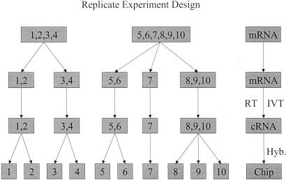
We study the measurement noise by replicate experiments in which gene expression levels of a cell line are measured multiple times. Two sources of experimental noise can be identified from the extracted mRNA to the final readout of the gene expression levels: the prehybridization target sample preparation steps and the hybridization and the subsequent readout processes (including staining and scanning). For simplicity, we refer to these two sources of noise as sample preparation noise and hybridization noise, respectively, throughout this article. To separate the noise sources caused by these two factors, we have carried out multiple replicate experiments, where at different stages of the experiment, the sample is divided equally into multiple aliquots, and the subsequent steps of the experiment are carried out independently. In this article, mRNA from cells of a human Burkitt's lymphoma cell line (Ramos) is used for the replicate experiments. Total RNA is extracted from the Ramos cells. The purified RNA sample subsequently is separated equally into several subgroups. Each subgroup independently goes through the target preparation steps, composed of the reverse transcription step and in vitro transcription (IVT) step. At the end of the target sample preparation, each of the subgroups is again split into several samples, each of which is independently hybridized to different Affymetrix U95A GeneChip arrays. The experimental design is shown schematically in Fig. 1. To have sound statistics and ensure the experimental statistics are independent of the starting mRNA, we have repeated the above replicate experiments with total RNA taken from two different cultures of the Ramos cells, as represented in Fig. 1, where experiments 1–4 and experiments 5–10 start from the different RNAs.

Fig 1.

Illustration of the replicate experiments setup. Two different mRNA samples are used, each being probed multiple times (replicates) with varying degrees of differences in measurement steps to separate the preparation error that occurred during the reverse transcription (RT) and IVT processes and the final hybridization (Hyb.) error.

Sample preparation starting from 5 μg total RNA, hybridization, staining, and scanning were performed according to the Affymetrix protocol. Unless indicated otherwise, our analysis uses the (average difference-based) expression values obtained by Affymetrix microarray suite (MAS) version 5.0 with all of the default parameters and target intensity set to 250. The expression values from earlier versions of MAS (versions 4.0 and 3.1) were used only for comparison purposes.

Results and Discussion

From the experiments described above, we obtain a gene expression value matrix {E_i,j}, where i = 1,2, … ,10 represents all of the experiments shown in Fig. 1 and j = 1,2, … , J labels all of the individual genes being probed. For the U95A chip we used, J ≈ 12,600. Due to the large variation in measured gene expression values, the analysis in this section is performed by using the logarithm of the expression level: θ_i,j = ln(E_i,j).

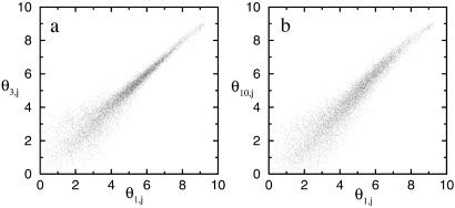
For a pair of experiments i₁ and i₂, the overall differences in gene expression can be visualized by plotting θ_i1,j versus θ_i2,j for all genes on the microarray. In Fig. 2, two pairs of experiments (1 and 3 and 1 and 10) are shown. The deviation of the scattered points from the diagonal line represents the difference between the two measured transcriptomes. Although Fig. 2 a and b appear similar, the reasons for the deviation of the expression values from the diagonal line are different. Experiments 1 and 3 measure mRNA levels of exactly the same sample, so the observed expression differences between these experiments are caused by measurement error alone. On the other hand, samples 1 and 10 are from different cultures of the cell line, so the measured expression value differences as shown in Fig. 2b contain the combined effect of the genuine gene expression differences between the two cultures together with differences caused by measurement error. Therefore, to correctly assess the statistical relevance of the measured gene expression differences between two experiments, such as 1 and 10, it is crucial to characterize the fluctuation caused purely by experimental measurement, such as the noise shown in Fig. 2a.

Fig 2.

The scatter plots of gene expression value pairs (,) for all genes j ∈ [1,J] and for: (a) experiments pair (1 and 3), where the deviation from the diagonal axis is caused purely by experimental error; (b) experiment pair (1 and 10), where true differences exist between the two transcriptomes.

Although experimental noise is known to be a feature of microarray experiments, only recently has it been studied systematically by replicate experiments (3, 4). In particular, for the oligonucleotide microarrays, Novak et al. (3) characterized the dispersion between two experiments by the SD of their corresponding gene expression levels. Using this measure of dispersion, they studied the different effects of experimental, physiological, and sampling variability, which provide important guidance for microarray experiment design. In this article, we focus on understanding how different experimental steps contribute to the total noise and what the possible mechanism for the noise could be. We also study the distribution of the noise in detail, which is used in devising a statistical method to determine differentially expressed genes.

To separate the different noise sources, we group all of the replicate experiment pairs into two groups. Group G₁ consists of all of the pairs that differ only in the hybridization step:

Group G₂ consists of all of the replicate experiment pairs that are carried out separately right after the extraction of the mRNA:

Although gene expression differences between pairs of experiments in G₂ represent the full experimental noise, G₁ has been constructed to extract the noise caused by hybridization alone. For reference, we also group all of the nonreplicate experiment pairs into group G₃ = {(i, j), 1 ≤ i ≤ 4, 5 ≤ j ≤10}.

The Noise Distribution.

It is evident from Fig. 2 that the noise depends strongly on the expression level. Therefore, an expression-dependent distribution function is needed to characterize the variability between replicates. Given two measured gene expression values, θ₁ and θ₂, for the same gene from two replicate experiments, the estimated value of the true expression level, θ̄, and the size of the measurement error, δθ, can be defined as: θ̄ = (θ₁ + θ₂)/2, δθ = (θ₁ −θ₂)/2. θ̄ is discretized with a relatively small bin size of 0.25 throughout this article to maintain a good resolution while having sufficient data points per bin. The results are insensitive to the exact choice of the bin size. For a given θ̄, the average of δθ between two experiments should be zero: 〈δθ|θ̄〉 = 0. Any significantly nonzero value of 〈δθ|θ̄〉 is caused by systematic experimental errors whose source is beyond the scope of our current study. This error typically appears as a departure from the diagonal of the scatter plots of Fig. 2. A hint of it can be seen at the higher values of Fig. 2b. Even though this was not a big problem for our data sets, we compensated for such error whenever it occurred by subtracting any nonzero 〈δθ|θ̄〉 from δθ for each replicate experiment pairs for all of the subsequent analysis.

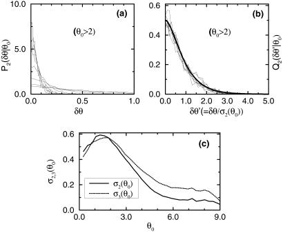
Within each group G_k (k = 1, 2), the distribution of δθ for a given θ̄ can be obtained from each pair of replicate experiments, these distributions are found to be highly consistent with each other (data not shown). To gain better statistics, we use the gene expression values from all of the pairs of replicate experiments in G_k to construct the noise distribution: P_k(δθ|θ₀) = Prob_k(δθ|θ̄ = θ₀). In Fig. 3a, the noise distribution functions for different values of θ₀ are shown. We use the second-order moment to quantify the strength of the noise and its dependence on the value of the expected expression level θ₀:

In Fig. 3c, we show the dependence of σ₂ on θ₀. For reference, we have calculated σ₃, the difference in gene expression between pairs of experiments in group G₃ in the same way as we calculated σ_1,2 and plotted it in Fig. 3c as well. It is interesting that σ₃ is consistently larger than σ₂ for θ₀ ≥ 2, indicating the existence of signal beyond noise even for the small differences between the same cell line from different cultures.

Fig 3.

The noise distribution functions at different values of mean expression values: θ₀ = 2,3,4,5,6,7,8,9 (a) before and (b) after rescaling by the SD σ₂(θ₀), which is shown in c. Only the positive region of δθ > 0 is shown in a and b for symmetry reasons. The rescaled distribution functions collapse onto a single curve well fitted by Φ(θ′) = 1/2exp(−x²/0.5 + 0.6|x|), plotted as the thick line shown in b.

For a given θ₀, we can define the rescaled noise δθ′ = δθ/σ_k(θ₀) and obtain the distribution function for δθ′: Q_k(δθ′|θ₀). We find that except for very small values of θ₀, the Q_k(δθ′|θ₀) collapse onto a single curve Φ(δθ′) independent of θ₀ and k, as shown in Fig. 3b (for k = 2 only). Equivalently, this means the distribution for δθ can be well approximated by:

for θ₀ ≥ 2, which includes more than 90% of the data. The rescaled distribution function is found to have an exponentially decaying tail in contrast with a Gaussian distribution. In fact, Φ(x) can be approximated very well by an empirical function Φ(x) ≈ 1/2 exp(−x²/0.5 + 0.6|x|) shown in Fig. 3b (thick solid line).

From Eq. 2, we see that all of the expression-dependent information in the noise is given by the variance σ(θ₀) for θ₀ ≥ 2. In the following two subsections, we focus on analyzing the dependence of the noise strength σ(θ₀) on the expression value.

Sample Preparation Noise.

To dissect the origins of noise, we divide the total measurement noise into two parts: the first is sample preparation noise δθ_prep caused by the prehybridization steps such as reverse transcription and IVT; the second is hybridization noise δθ_hyb. For replicate pairs in group G₁ and G₂, the noise can be expressed, respectively, as: δθ₁ = δθ_hyb, δθ₂ = δθ_prep + δθ_hyb. Assuming the two sources of noise are independent of each other, their variances can be obtained by: σ = 〈δθ〉 = σ, σ = 〈δθ〉 = σ − σ, where σ can be computed from Eq. 1.

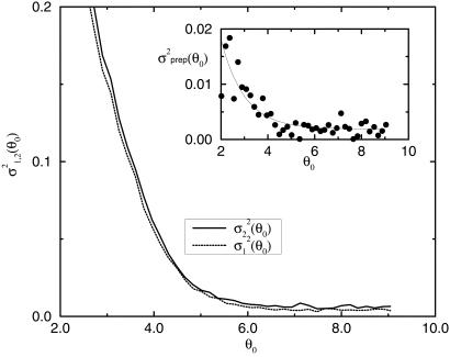
In Fig. 4, we show σ(θ₀) (dotted line) and σ(θ₀) (solid line) versus the expected value of the expression level θ₀. Although the difference between σ₂ and σ₁ is small in comparison with σ₂, σ₁(θ₀) is consistently smaller than σ₂(θ₀) for all of the values of θ₀ ≥ 2. This should be so because the difference between σ₂ and σ₁ accounts for the sample preparation noise: this difference, albeit small, is real.

Fig 4.

The dependence of the noise strength σ, on the expected values of the gene expression for replicates in groups G₁ and G₂. (Inset) The variance of the sample preparation noise σ = σ − σ is shown. σ_prep has very weak dependence on the expression value for the large expression levels θ₀ ≥ 4.0 and can be fitted by 1.9 × 10⁻³ + 0.12 × e^−θ₀ for θ₀ ≥ 2.

We have plotted the dependence of σ versus θ₀ in Fig. 4 Inset. We find that the dependence of σ on the expression level θ₀ can be well approximated by:

The constant first term dominates the sample preparation noise for expression values θ₀ ≥ 4.

To understand the possible mechanisms for such noise behavior as shown in Eq. 3, it is convenient to translate the above noise strength in θ (= ln(E)) to the noise strength in intensity E: σ(E₀) ≡ 〈δE²〉 ≈ E〈δθ²〉, where E₀ = exp(θ₀) and δE = E − E₀. By using the numerical fit for σ, the variance of the sample preparation noise δE_prep, σ, can written as:

The two terms in the above expression represent two independent sources of noise, which we discuss in the following.

For the first term, δE_prep is proportional to the gene expression E₀ itself. To understand this term, it is important to realize that during sample preparation the mRNA is first reverse-transcribed into cDNA, and cRNA is subsequently generated from cDNA by IVT. The number of RNA molecules is amplified during the IVT, i.e., N_cRNA = A × N_mRNA, where A is the amplification rate and N_mRNA, N_cRNA are the numbers of mRNA and cRNA molecules, respectively. A varies between one sample preparation process and another due to fluctuations in the reaction conditions, including fluctuation due to handling of the sample (human factors). The fluctuation of A between different sample preparation processes, denoted as δA, leads to a fluctuation in N_cRNA of the form δA × N_mRNA. Because N_mRNA is proportional to E₀, the first term in Eq. 4 can thus be explained by the fluctuation in A. Furthermore, σ_A, the SD of A, can be estimated: σ_A ≡ 〈δA²〉^1/2 ≈ (1.9 × 10⁻³)^1/2Ā, where Ā is the mean amplification rate. Assuming a typical value of Ā around 100 (5), we have σ_A ∼ 4.4.

For the second term in Eq. 4, δE_prep is only proportional to the square root of E₀, which is thus indicative of a Poisson-like noise. Such Poisson-like noise in the sample preparation may arise naturally from the probabilistic nature of the amplification process (IVT).

The accuracy of the sample preparation process inevitably depends on human factors, whose influence is difficult to estimate. Our result here can be best viewed as an upper limit for the noise caused by the intrinsic chemical processes involved in the sample preparation.

Hybridization Noise.

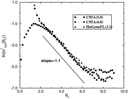
Most of the total measurement error comes from the hybridization noise, which depends strongly on the expression level (see Fig. 4). For expression level θ₀ ≥ 2, the hybridization noise σ decreases rapidly with increasing expression level as shown in Fig. 5, where ln(σ) is plotted versus θ₀. Empirically, σ can be fitted by:

with β = 4.6 ± 0.2 and γ = 1.1 ± 0.1 for the region 3.2 ≤ θ₀ ≤ 6.2, before saturating to a constant (3.2 × 10⁻³).

Fig 5.

Logarithm of the hybridization noise versus the expression level for our data obtained by different versions of Affymetrix MAS. •, Results from MAS 5.0; ▪, results from MAS 4.0. We have also calculated the noise strength from Lemon et al.'s replicate data (see ref. 6), which was performed with a different type of GeneChip array (HuGeneFL), with a different type of sample (human fibroblast cells) and by using MAS 3.1. The agreement between the three results indicates a certain universality of the noise characteristics in the region 3.0 ≤ θ₀ ≤ 7.0, where the variance of the noise decays exponentially (see text).

Also in Fig. 5, we have included the hybridization noise calculated by using expression values obtained from MAS version 4.0 [for 4.0 and earlier versions of MAS, θ_ij is defined as: θ_ij ≡ ln(max(E_ij, E_c)), where we choose a small E_c = 0.1 as a cutoff in avoiding negative expression values]. It is reassuring to see the results from the old and new versions of the software are consistent in the high-expression value region. The different behavior at low expression values reflects the major difference between versions 4.0 and 5.0 in dealing with negative differences between perfect match and mismatch probe pairs. This difference may be irrelevant because most of the genes with low expression values θ₀ ≤ 3 are considered to be absent from both versions of the software (see Fig. 6b).

Fig 6.

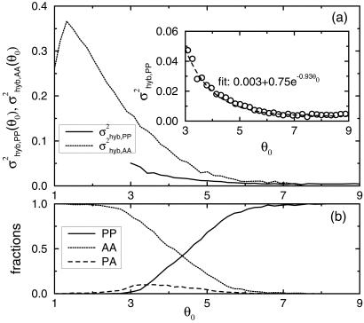
(a) The overall hybridization noise (black line) is decomposed into two parts: the hybridization noise for genes that are labeled by MAS 5.0 as present (σ_hyb,PP, solid line) or absent (σ_hyb,AA, dotted line). (Inset) σ is fitted by 3.2 × 10⁻³ + 0.75 × exp(−0.93θ₀). For reference, the fractions of the PP, PA, and AA pairs in all of the replicate experiments at a given mean expression value θ₀ are plotted in b.

To examine the robustness of the hybridization noise characteristics, we have also calculated the hybridization noise strength (σ′_hyb)² for nine pairs of replicate experiments (6), which were performed with a different type of Affymetrix GeneChip array (HuGeneFL), with a different type of cell (human fibroblast cells) and in a different laboratory. The results are shown in Fig. 5 along with our data. It is remarkable that the exponentially decaying part of the hybridization noise seems universal regardless of the type of genechip and the sample being used. Notice also the agreement of the noise behavior in the full θ₀ range between our data generated with MAS 4.0 and the independently generated data of ref. 6 with MAS 3.1, which uses the same analysis algorithm as MAS 4.0. This observation indicates that the noise as characterized in the present analysis seems to show a degree of universality; more work is needed in confirming this behavior.

Noise in the hybridization signal can come from fluctuations in both the target molecule binding and cross-hybridization (nonspecific binding), which may have different behaviors. To roughly separate between specific and nonspecific hybridization, we use the Affymetrix “present” (PP) and “absent” (AA) calls. In particular, we calculate the noise strengths σ and σ for only those genes whose calls are both present and both absent for the replicate experiment pair from G₁. The results are shown in Fig. 6a. For reference, we also plot the fractions of the PP, AA, and PA pairs for a given mean expression value θ₀ in Fig. 6b. From Fig. 6a, it becomes clear that the noise characteristics are different for σ and σ. This is most evident in the region 3 ≤ θ₀ ≤ 6, where PP pairs and AA pairs are both populated (see Fig. 6b). Their different behavior suggests that σ_hyb,PP and σ_hyb,AA have different origins.

For σ, we can fit the PP hybridization noise strength with

for θ₀ ≥ 3.0 and with α_PP = 3.2 × 10⁻³ ± 2.0 × 10⁻⁴, β_PP = 0.75 ± 0.1, and γ_PP = 0.93 ± 0.04 as shown in Fig. 6a Inset. The origins of the two noise terms in Eq. 6 may be understood as follows. In general, for a gene with a present call, the final expression readout E should be proportional to N_cRNA, the number of cRNA molecules of the gene: E = qN_cRNA. However, the proportional factor q, which depends on the hybridization and the subsequent readout processes, can vary between different gene chips [for example, due to differences in purity of the probes on different gene chips (7)]. Such fluctuation in q between different experiments can give rise to the (constant) first term in Eq. 6. The second term in Eq. 6, with γ_PP ∼ 1, indicates a Poisson-like noise (see earlier discussion of the sample preparation noise). Such Poisson-like noise may arise naturally from the probabilistic nature of the hybridization and the subsequent readout processes.

For σ_hyb,AA, it cannot be fitted with any simple form that would allow speculations about its origin. The best fit with an exponential function in the region 2 ≤ θ₀ ≤ 5.0 is (not shown in Fig. 6a): σ ∼ β_AAe^{−γ_AAθ₀} with β_AA = 1.3 ± 0.1 and γ_AA = 0.72 ± 0.1. Indeed, it is not clear what the expression intensity means when the gene is deemed absent by the Affymetrix call. Most likely, the intensity value and its fluctuation, if meaningful at all, are affected by cross-hybridization. The final intensity values and their fluctuations depend very much on the way one deals with negative differences between perfect match and mismatch probe pairs, which occur most frequently in the absent genes. This is consistent with our finding (data not shown) that σ_hyb,AA changes significantly when we use the intensity values from MAS 4.0 instead of MAS 5.0, whereas the change in σ_hyb,PP between the two versions is minimal.

USE-Fold: A Method for Uniform Significance of Expression Fold Change.

The results presented in the previous sections can be used to design a method for determining the statistical relevance of gene expression changes. The idea is simply that the fold change experienced by a gene under different biological conditions has to be larger than the fold change expected from the noise. We shall use the full noise distribution function discussed previously to evaluate the significance of the difference between a pair of gene expressions (θ₁,θ₂) for the same gene but different experiments. By using the fluctuation between replicate experiment pairs in G₂ as the null hypothesis, a gene expression-dependent p value can be defined as:

where Δθ₀ = |θ₁ − θ₂|/2, θ₀ = (θ₁ + θ₂)/2.

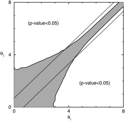
For θ₀ ≥ 2, we can use Eq. 2, and the p value can be expressed simply as a function of the signal-to-noise ratio R ≡ Δθ₀/σ₂(θ₀): p(θ₁,θ₂|θ₀) = 2∫ Φ(x)dx. In Fig. 7, the contour lines for p(θ₁,θ₂|θ₀) = 0.05 are shown together with two lines corresponding to a uniform 2-fold expression value change [|θ₁ − θ₂| = ln(2)]. This clearly shows that given a fixed confidence level (p value = 0.05), a requirement of a uniform 2-fold expression change is too stringent for the high expression level, while being inadequate for the low expression level (θ₀ ≤ 4). In fact, given the strong expression level dependence of the noise, no significance criterion based solely on the expression fold change is appropriate. Instead, to guarantee a fixed level of statistical relevance p₀, one can enforce a uniform (i.e., expression level independent) lower bound on the signal-to-noise ratio R ≥ R₀(p₀).

Fig 7.

The contour line of p value equal to 0.05. Any pair of expression values (θ₁,θ₂) outside the shaded area represents differently expressed genes beyond experimental noise with a p value of 0.05 or smaller. The two dotted lines represent 2-fold expression changes.

The above discussion suggests the following method of selecting differently expressed genes with user-defined statistical significance:

• Evaluate the noise level from replicate experiments such as those in group G₂. Ideally, each laboratory should carry out its replicate experiments to determine the noise level. If this is not possible, the results of this article may be used with some degree of confidence, as we have shown consistency between two sets of replicate data produced in different laboratories (our data and that of ref. 6, see Fig. 5).

• After obtaining σ₂(θ₀) from the previous step, pick a significance level p₀, and compute the corresponding threshold for the signal-to-noise ratio R₀ such that p₀ = 2∫Φ(x)dx, where Φ(x) is the noise distribution function. Using the empirical form of φ(x) = 1/2 exp(−x²/0.5 + 0.6|x|) found in this article, for significance level p₀ = 0.05, we find the corresponding R₀ ≈ 2.1.

• Given two expression values E₁ and E₂, corresponding to the fluorescence intensity of the same gene from different gene chips, compute θ₁ = ln(E₁) and θ₂ = ln(E₂), and define θ₀ = (θ₁ + θ₂)/2. The fold change φ = max(E₁/E₂, E₂/E₁) is statistically significant with a p value less or equal than p₀ if the signal-to-noise ratio ln(φ)/(2σ₂(θ₀)) ≥ R₀.

To demonstrate the utility of this method, we have applied it to discover differentially expressed genes between two developmentally distinct types of B lymphocytes, a centroblast (CB) and a naive (N) B cell (see Tables 1 and 2, Fig. 8, and additional Text, which are published as supporting information on the PNAS web site, www.pnas.org, for details). A total of 1,490 genes were found to change more than 2-fold in their expression values and have at least one present call in either of the two experiments. However, more than 10% of these genes do not pass the USE-Fold noise test with p₀ = 0.05. For example, one gene (GenBank accession no. AA143021) has present calls in both experiments with expression values E₁ = 48.3 and E₂ = 21.7 for CB and N, respectively. Even though the fold change φ = E₁/E₂ = 2.23 is greater than 2, at their mean (logarithmic) expression level of θ₀ = (ln(E₁) + ln(E₂))/2 = 3.48, the noise level is also large, σ₂(θ₀) = 0.32 (see Fig. 4) and the signal-to-noise ratio ln(φ)/(2σ₂(θ₀)) = 1.25 is smaller than R₀ = 2.1. Therefore, this gene cannot be considered to be differentially expressed with high confidence by just these two experiments. To test whether or not such gene is differentially expressed between the two types of B cell, more experiments need to be done to average out the effect of the random experimental noise (8). This is necessary particularly for genes with low expression, because the relative noise is much larger at low expression levels.

All of the data used in this article and free software implementing the USE-Fold method can be found at our web site (www.research.ibm.com/FunGen/index.html).

Conclusions

In this article, we have systematically studied the experimental noise characteristics of Affymetrix GeneChip microarray experiments. By designing replicate experiments that differ from each other at different stages of the experiments, we are able to decompose the total experimental noise into two parts: the sample preparation (prehybridization) noise and the hybridization (including the subsequent readout processes) noise. We have characterized these two sources of noise quantitatively, and in particular, their dependence on the gene expression level itself. For the sample preparation noise, we find that it is dominated by an expression-independent constant and is in general much smaller than the hybridization noise. For the hybridization noise, except for a small constant component, the noise strength is found to depend strongly on the expression level. Specifically, for the genes labeled by the Affymetrix call as present, the dependence of the hybridization noise strength on the expression indicates a Poisson-like noise, in accordance with the probabilistic nature of the hybridization process; for the absent genes, however, the hybridization noise characteristics does not have a simple explanation, because the noise and even the gene expression readout itself are affected by cross-hybridization.

Overall, the importance of this work is 2-fold. First, our study provides a quantitative measure of the experimental noise, which served us as a base for designing a simple method for determining statistical meaningful biological information from gene expression microarray data. Second, our study provides insight into the sources of the noise by decomposing the noise according to the individual steps of the genechip experiment. The insights gained from this study may help to further reduce the errors arising in DNA microarray experiments.

Abbreviations

• IVT, in vitro transcription

• MAS, microarray suite

References

- 1.Lockhart D. J. & Winzeler, E. A. (2000) Nature 405, 827-836. [DOI] [PubMed] [Google Scholar]
- 2.Brown P. O. & Botstein, D. (1999) Nat. Genet. 21,Suppl., 33-37. [DOI] [PubMed] [Google Scholar]
- 3.Novak J. P., Sladek, R. & Hudson, T. J. (2002) Genomics 79, 104-113. [DOI] [PubMed] [Google Scholar]
- 4.Lee M.-L. T., Kuo, F. C., Whitemore, G. A. & Sklar, I. (2000) Proc. Natl. Acad. Sci. USA 97, 9834-9839. [DOI] [PMC free article] [PubMed] [Google Scholar]
- 5.Lockhart D. J., Dong, H., Byrne, M. C., Follettie, M. T., Gallo, M. V., Chee, M. S., Mittmann, M., Wang, C., Kobayashi, M., Hortan, H. & Brown, E. L. (1996) Nat. Biotechnol. 14, 1675-1680. [DOI] [PubMed] [Google Scholar]
- 6.Lemon, W. J., Palatini, J. J. T., Krahe, R. & Wright, F. A. (2001) preprint, http://thinker.med.ohio-state.edu/projects/fbss/index.html.
- 7.Forman J. E., Walton, I. D., Stern, D., Rava, R. P. & Trulson, M. O. (1997) Am. Chem. Soc. Symp. Ser. 682, 2208-2228. [Google Scholar]
- 8.Pan W., Lin, J. & Le, C. T. (2002) Genome Biol. 3, 1-10. [DOI] [PMC free article] [PubMed] [Google Scholar]
Associated Data
This section collects any data citations, data availability statements, or supplementary materials included in this article.