Evaluating Statistical Significance in Two-Stage Genomewide Association Studies

Abstract

Genomewide association studies are being conducted to unravel the genetic etiology of complex human diseases. Because of cost constraints, these studies typically employ a two-stage design, under which a large panel of markers is examined in a subsample of subjects, and the most-promising markers are then examined in all subjects. This report describes a simple and efficient method to evaluate statistical significance for such genome studies. The proposed method, which properly accounts for the correlated nature of polymorphism data, provides accurate control of the overall false-positive rate and is substantially more powerful than the standard Bonferroni correction, especially when the markers are in strong linkage disequilibrium.

A decade ago, Risch and Merikangas (1996) suggested that genetic variants predisposing to complex human diseases could be identified through genomewide association scans involving hundreds of thousands or more markers and thousands of subjects. With the recent availability of genomewide surveys of genetic variants (The International SNP Map Working Group 2001; Hinds et al. 2005; The International HapMap Consortium 2005) and the rapid decrease in SNP genotyping costs, this vision has become a real possibility. Indeed, numerous genomewide association studies for a range of disorders are being planned or are already underway.

Despite recent advances in high-volume genotyping technology, it is still prohibitively expensive to genotype hundreds of thousands of markers in thousands of subjects. Thus, most genomewide association studies adopt a two-stage design: in the first stage, a dense set of SNP markers across the genome is genotyped and tested using a fraction of the available subjects, and, in the second stage, the most-promising markers are genotyped in the remaining subjects and tested using all subjects (Satagopan et al. 2002, 2004; Satagopan and Elston 2003; Maraganore et al. 2005; Thomas et al. 2005; Skol et al., in press).

Assessing statistical significance in such two-stage genome studies presents an important challenge. The current practice is to use the Bonferroni correction based on the total number of markers tested in the first stage (Maraganore et al. 2005; Thomas et al. 2005). This strategy is punitively conservative for two reasons. First, it assumes that none of the markers eliminated in stage 1 would reach statistical significance if they were genotyped and tested in stage 2. Second, it assumes that the test statistics are independent over all markers. The first assumption was relaxed by Skol et al. (in press). The second assumption fails when markers are in linkage disequilibrium (LD). The ENCODE data from the HapMap Project reveal that SNPs are typically in complete LD with several nearby SNPs and in strong LD with many others; thus, the Bonferroni correction is highly conservative (The International HapMap Consortium 2005).

In this report, I show how to properly incorporate the two-stage sampling and the correlation structure of the test statistics into the evaluation of statistical significance. The strategy relies on the fact that the statistics used in association testing can be represented by the so-called efficient score functions, which are sums of independent terms (see appendix A). This fact implies that the statistics are jointly normal in large samples, both over the markers and between the two stages, with correlations that can be estimated empirically from the data. I develop an efficient Monte Carlo algorithm to evaluate this joint distribution, providing appropriate thresholds for declaring statistical significance.

Suppose that a total of m markers are genotyped and tested on n₁ subjects in stage 1, and the most-promising markers are genotyped in the remaining n₂=n-n₁ subjects and tested using all n subjects in stage 2. All subjects are assumed to be unrelated. For s=1,2 and j=1,…,m, the test statistic for testing the mth marker in the sth stage can be written in the following form or can be approximated by the statistic of the following form:

where

U_ji involves only the data from the ith subject,

and

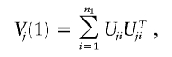
Note that U_j pertains to the efficient score function, and V_j is the covariance matrix of U_j (see appendix A). In most situations,

where Y_i is the phenotypic value of the ith subject, X_ji is the genotype score for the jth marker of the ith subject, and μ_y and μ_j are the population means of Y_i and X_ji, respectively. In the actual calculations of T_j(s), μ_y and μ_j are replaced with the sample means.

Under the null hypothesis of no association, U_j(s) is approximately normal with mean zero and covariance matrix V_j(s) in large samples, so T_j(s) has an approximate χ² distribution with d df, where d is the dimension of U_j(s). In addition, [U₁(1),…,U_m(1),U₁(2),…,U_m(2)] is approximately multivariate normal with mean zero and covariance matrices

and

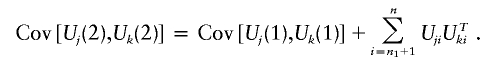Note that Cov(Z₁,Z₂+Z₃)=Cov(Z₁,Z₂) if Z₁ and Z₃ are uncorrelated. The values of U_ji (i=n₁+1,…,n) are unknown unless the jth marker is genotyped in stage 2. However,

can be estimated by

provided that the subjects are randomly chosen for genotyping in stage 1.

I derive a simple and efficient Monte Carlo procedure to evaluate the joint distribution of [U₁(1),…,U_m(1),U₁(2),…,U_m(2)]. Define

and

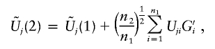where G₁,…,G_n1,G^′₁,…,G^′_n1 are independent standard normal random variables. Also, define

Conditional on the observed data, is multivariate normal with mean zero and (approximately) the same covariance matrix as [U₁(1),…,U_m(1),U₁(2),…,U_m(2)]. Thus, one can use the joint distribution of to approximate that of [T₁(1),…,T_m(1),T₁(2),…,T_m(2)].

Suppose that the jth marker is selected for genotyping in stage 2 if T_j(1)>c₁, where c₁ is chosen to achieve a certain level of statistical significance or to yield a desired proportion of markers for stage 2 testing. The null hypothesis of no association between the jth marker and disease is rejected if T_j(1)>c₁ and T_j(2)>c₂, where c₂ is chosen so that, under the global null hypothesis of no association,

where α is the nominal type I error rate or significance level. One can approximate this equation by

The probability on the left-hand side of equation (1) is estimated by generating a large number, say 10,000, of realizations of and .

Given c₁ and α, one can use equation (1) to determine c₂. This calculation can be done through a bisection search based on a single set of realizations of and . In practice, c₂ on the left-hand side of equation (1) is replaced with the observed value of T_j(2), and significant association with the jth marker is declared if the resulting probability is <α.

To assess the performance of the proposed method, I simulated 10,000 SNPs with minor-allele frequencies of 0.3 and varying degrees of LD. I set the disease prevalence in the population to be ∼5%. Under the null hypothesis, none of the SNP markers was associated with disease. Under the alternative hypothesis, the minor allele of SNP 5,000 had a dominant effect with a relative risk of 1.5. I selected 1,000 cases and 1,000 controls and used the Pearson χ² statistic under the dominant model to test the association between each SNP and disease status. I set the nominal significance level at 0.05.

Figure 1 displays the results for the two-stage design, under which 50% of the cases and controls are genotyped in stage 1; c₁ was set at 3, so that ∼10% of the markers are selected for genotyping in stage 2. The results for other designs are similar and thus omitted. The empirical type I error rate pertains to the probability of finding any association under the null hypothesis, and the empirical power pertains to the probability of identifying SNP 5,000 under the alternative hypothesis. Each of these probabilities was estimated from 1,000 simulated data sets; for each data set, the Monte Carlo evaluation was based on 10,000 normal samples.

Figure 1.

Empirical type I error rate and power at the nominal significance level of 0.05. The red and orange curves correspond to the type I error and power of the proposed method, respectively, and the blue and green curves correspond to the type I error and power of the Bonferroni correction, respectively. The X-axis pertains to the squared correlation coefficient, r², between two adjacent markers, which varies from 0.5 to 0.99.

As shown in figure 1, the proposed method maintains its type I error near the nominal level, whereas the Bonferroni correction is conservative. The type I error rates of the proposed method are ∼0.052, 0.055, and 0.050 when the squared correlation coefficient, r², between two adjacent markers is 0.5, 0.9, and 0.99, respectively. By contrast, the corresponding type I rates based on the Bonferroni correction are ∼0.037, 0.022, and 0.002.

The proposed method is considerably more powerful than the Bonferroni correction, especially when the markers are in strong LD. The power of the proposed method is ∼75%, whereas that of the Bonferroni correction is ∼65%, when r² between two adjacent markers is 0.9; the corresponding power estimates are 85% and 60% when r² is 0.99. For the Bonferroni correction to achieve the same power as that of the proposed method, the sample sizes would need to be increased by ∼15% and 30% when the r² values between two adjacent markers are 0.9 and 0.99, respectively. Thus, the power advantages of the proposed method have important implications.

In the studies above, LD was created by allowing the SNP allele frequencies of each marker to depend on those of the preceding marker, so that the LD decays exponentially as the intermarker distance increases. When r² is 0.9 between two adjacent markers, the value of r² is 0.8 between every second marker and 0.3 between SNPs that are 10 markers apart; when r² is 0.99 between two adjacent markers, the value of r² is 0.98 between every second marker and 0.8 between SNPs that are 20 markers apart.

To generate more-realistic LD structures, I considered the HapMap data (The International HapMap Consortium 2005). I simulated data in the same manner as in the studies above, except that the genotypes were sampled from the white phasing data in the ENCODE region of chromosome 4, which consists of 1,393 SNPs. Under the null hypothesis of no association, the type I error rates were found to be ∼0.047 and 0.009 for the proposed and Bonferroni methods, respectively. Under the alternative hypothesis that SNP 1,100, which has a minor-allele frequency of ∼0.2, had a dominant effect with a relative risk of 1.5, the power was ∼0.91 for the proposed method, compared with 0.78 for the Bonferroni correction.

The results in figure 1 pertain to 10,000 SNPs, which is approximately the number of markers on a single chromosome in the currently available 100K–500K SNP platforms. Since the test statistics are generally uncorrelated among the chromosomes, the proposed method can be applied to each chromosome separately. It is unclear whether one should adjust for multiple comparisons among chromosomes when hundreds of thousands or more markers are tested. It is perhaps more sensible to control a few (say, 10–20) false positives rather than a single one in such massive-scale hypothesis testing (Lehmann and Romano 2005).

The above studies were concerned with single-locus effects. The proposed method is certainly applicable to multilocus searches, including interactions and haplotype effects (Epstein and Satten 2003). The method is also potentially useful for complex multistage studies.

This method combines the raw data from the two stages in the final analysis. An alternative approach is to combine the two test statistics (i.e., to sum the two standardized statistics) (Skol et al., in press). It is trivial to modify this method for the combined test statistics, provided that the subjects are randomly selected for genotyping in stage 1. However, a major motivation for combining the two test statistics is to allow for heterogeneity between the first-stage and second-stage samples. The work of Zaykin et al. (2002) and Dudbridge and Koeleman (2004) can also be extended to two-stage studies through this Monte Carlo approach. Although I have focused on studies of unrelated individuals, the proposed method can be adapted to family studies by changing “subject” to “family” in the description.

Because of the two-stage sampling, the method described here is different from that of Lin (2005a, 2005b). In particular, the new Monte Carlo procedure circumvents the problem that the genotype data are unobserved for those markers eliminated in the first stage.

Unlike for single-stage studies, it is not possible to evaluate statistical significance for two-stage studies by permutation. If the value of T_j(1) based on the original data does not exceed c₁, then the jth marker is not genotyped in stage 2. When the data are permuted, the value of T_j(1) based on the permuted data may exceed c₁. In that case, one needs to evaluate T_j(2) on the basis of the permuted data, but that evaluation is not possible because the jth marker is missing in all n₂ subjects.

The proposed method provides an essential ingredient for designing genomewide association studies. In the design stage, one would simulate the genotype data for the specific SNPs to be tested and use equation (1) to determine c₂. One would then determine the power by evaluating the probabilities of true detection for various relative risks through simulation.

I found that two-stage designs in which ∼50% of the available subjects are genotyped in stage 1 and the top 1%–10% of the markers are genotyped in stage 2 are nearly as powerful as the single-stage design that genotypes all markers in all subjects (data not shown). Similar findings were reported elsewhere for independent test statistics (Satagopan and Elston 2003; Skol et al., in press). Thus, two-stage designs are highly cost effective. With the Bonferroni correction, the penalty is proportional to the number of markers tested in stage 1, regardless of the marker density. By contrast, the proposed method properly accounts for the actual correlations of SNPs and does not unfairly penalize SNP platforms with very high density.

A computer program that implements the proposed method is freely available at the author's Web site (see Web Resource section). The computing time is linear in relation to the number of markers and the number of subjects. The analysis for a typical genome scan (100K–500K markers and 1,000–5,000 subjects) can be completed in a short amount of time on any high-performance computer.

Appendix A: Score Statistics

For quantitative traits, it is natural to consider the linear regression model

where X_ji is the ith subject’s genotype score for the jth marker and ε_i is normal with mean 0 and variance σ². For simplicity of description, the dependence of the parameters on j is suppressed. Under the additive model, X_ji denotes the number of minor alleles that the ith subject has; under the dominant (or recessive) model, X_ji indicates, with values of 1 and 0, whether or not the ith subject has at least one minor allele (or, for the recessive model, two minor alleles); under the codominant model, X_ji consists of two components indicating one and two minor alleles. For dichotomous traits, it is common to employ the logistic regression model

One is interested in testing the null hypothesis H₀:β=0 against the alternative hypothesis H₁:β≠0 at every marker. The parameters μ and σ² in model (A1) and ν in model (A2) are nuisance parameters, which are denoted by η. There are three asymptotically equivalent test statistics: the Wald statistic, the likelihood-ratio statistic, and the score statistic. Here, it is convenient to work with score statistics.

The log-likelihood function for (β,η) at the jth marker is , where l_ji(β,η) pertains to the contribution from the ith subject. Let U_β,ji(β,η)=∂l_ji(β,η)/∂β and U_η,ji(β,η)=∂l_ji(β,η)/∂η. The score statistic for testing H₀:β=0 takes the form

where is the (restricted) maximum-likelihood estimator of η under H₀—that is, the solution to the equation . Note that U_j is the score function for β evaluated at β=0 and and is not a sum of independent terms for a given j. It follows from the Taylor series expansions and the law of large numbers that n^-1/2U_j has the same asymptotic distribution as , where

and Σ_βη(β,η) and Σ_ηη(β,η) are the limits of n^-1∂²l_j(β,η)/∂β∂η and n^-1∂²l_j(β,η)/∂η² as n goes to infinity (Cox and Hinkley 1974, section 9.3(iii)). One calls U_ji the ith subject’s efficient score function. Under both models (A1) and (A2),

where μ_y and μ_j are the population means of Y_i and X_ji, respectively. Since U_ji involves only the observations from the ith subject, U_ji are independent zero-mean random vectors for any given j. Thus, it follows from the multivariate central limit theorem that, under the null hypothesis of no association, n^-1/2(U₁,…,U_m) is asymptotically multivariate normal with mean 0 and with as the covariance matrix between the jth and kth markers.

In the actual calculations of the test statistics, the unknown parameters in U_ji are replaced with the (restricted) maximum-likelihood estimators. Since by the definition of , the replacement of η with in U_ji yields , which is consistent with the definition of the score statistic given in equation (A3). It can be shown that, under model (A1) with a dichotomous genotype score,

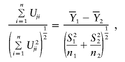where n₁ and n₂ are the numbers of subjects in the two groups and and (S²₁,S²₂) are the sample means and sample variances in the two groups. This is, of course, the well-known two-sample t statistic. Likewise, the familiar Pearson χ² statistics can be generated under model (A2).

The above description pertains to single-stage studies. However, all the results can be extended to two-stage designs in an obvious manner.

References

- Cox DR, Hinkley DV (1974) Theoretical statistics. Chapman and Hall, New York [Google Scholar]
- Dudbridge F, Koeleman BPC (2004) Efficient computation of significance levels for multiple associations in large studies of correlated data, including genomewide association studies. Am J Hum Genet 75:424–435 [DOI] [PMC free article] [PubMed] [Google Scholar]
- Epstein MP, Satten GA (2003) Inference on haplotype effects in case-control studies using unphased genotype data. Am J Hum Genet 73:1316–1329 [DOI] [PMC free article] [PubMed] [Google Scholar]
- Hinds DA, Stuve LL, Nilsen GB, Halperin E, Eskin E, Ballinger DG, Frazer KA, Cox DR (2005) Whole-genome patterns of common DNA variation in three human populations. Science 307:1072–1079 10.1126/science.1105436 [DOI] [PubMed] [Google Scholar]
- Lehmann EL, Romano JP (2005) Generalizations of the familywise error rate. Ann Stat 33:1138–1154 10.1214/009053605000000084 [DOI] [Google Scholar]
- Lin DY (2005a) An efficient Monte Carlo approach to assessing statistical significance in genomic studies. Bioinformatics 21:781–787 10.1093/bioinformatics/bti053 [DOI] [PubMed] [Google Scholar]
- ——— (2005b) On rapid simulation of P values in association studies. Am J Hum Genet 77:513–514 [DOI] [PMC free article] [PubMed] [Google Scholar]
- Maraganore DM, de Andrade M, Lesnick TG, Strain KJ, Farrer MJ, Rocca WA, Pant PVK, Frazer KA, Cox DR, Ballinger DG (2005) High-resolution whole-genome association study of Parkinson disease. Am J Hum Genet 77:685–693 [DOI] [PMC free article] [PubMed] [Google Scholar]
- Risch N, Merikangas K (1996) The future of genetic studies of complex human diseases. Science 273:1516–1517 [DOI] [PubMed] [Google Scholar]
- Satagopan JM, Elston RC (2003) Optimal two-stage genotyping in population-based association studies. Genet Epidemiol 25:149–157 10.1002/gepi.10260 [DOI] [PMC free article] [PubMed] [Google Scholar]
- Satagopan JM, Venkatraman ES, Begg CB (2004) Two-stage designs for gene-disease association studies with sample size constraints. Biometrics 60:589–597 10.1111/j.0006-341X.2004.00207.x [DOI] [PMC free article] [PubMed] [Google Scholar]
- Satagopan JM, Verbel DA, Venkatraman ES, Offit KE, Begg CB (2002) Two-stage designs for gene-disease association studies. Biometrics 58:163–170 10.1111/j.0006-341X.2002.00163.x [DOI] [PMC free article] [PubMed] [Google Scholar]
- Skol AD, Scott LJ, Abecasis GR, Boehnke M. Forget replication: joint analysis is more efficient for genomewide association studies. Nat Genet (in press) [DOI] [PubMed] [Google Scholar]
- The International HapMap Consortium (2005) A haplotype map of the human genome. Nature 437:1299–1320 10.1038/nature04226 [DOI] [PMC free article] [PubMed] [Google Scholar]
- The International SNP Map Working Group (2001) A map of human genome sequence variation containing 1.42 million single nucleotide polymorphisms. Nature 409:928–933 10.1038/35057149 [DOI] [PubMed] [Google Scholar]
- Thomas DC, Haile RW, Duggan D (2005) Recent developments in genomewide association scans: a workshop summary and review. Am J Hum Genet 77:337–345 [DOI] [PMC free article] [PubMed] [Google Scholar]
- Zaykin DV, Zhivotovsky LA, Westfall PH, Weir BS (2002) Truncated product method for combining P-values. Genet Epidemiol 22:170–185 10.1002/gepi.0042 [DOI] [PubMed] [Google Scholar]