Water and heat transport in hilly red soil of southern China: II. Modeling and simulation

Abstract

Simulation models of heat and water transport have not been rigorously tested for the red soils of southern China. Based on the theory of nonisothermal water-heat coupled transfer, a simulation model, programmed in Visual Basic 6.0, was developed to predict the coupled transfer of water and heat in hilly red soil. A series of soil column experiments for soil water and heat transfer, including soil columns with closed and evaporating top ends, were used to test the simulation model. Results showed that in the closed columns, the temporal and spatial distribution of moisture and heat could be very well predicted by the model, while in the evaporating columns, the simulated soil water contents were somewhat different from the observed ones. In the heat flow equation by Taylor and Lary (1964), the effect of soil water evaporation on the heat flow is not involved, which may be the main reason for the differences between simulated and observed results. The predicted temperatures were not in agreement with the observed one with thermal conductivities calculated by de Vries and Wierenga equations, so that it is suggested that K _h, soil heat conductivity, be multiplied by 8.0 for the first 6.5 h and by 1.2 later on. Sensitivity analysis of soil water and heat coefficients showed that the saturated hydraulic conductivity, K _S, and the water diffusivity, D(θ), had great effects on soil water transport; the variation of soil porosity led to the difference of soil thermal properties, and accordingly changed temperature redistribution, which would affect water redistribution.

INTRODUCTION

It is recognized that the transfer of soil moisture and heat occur simultaneously and are interrelated. Since the 1950s, many models have been developed, based on two nonisothermal water-heat coupled models by Philip and de Vries (1957) and Taylor and Lary (1964), respectively. In China, some researches on modeling coupled transfer of soil moisture and heat have also been conducted on the arid soils in northern China (Kang et al., 1993; Guo and Li, 1997; Hu et al., 1992; Ren et al., 1998), but only little preliminary work has been done on red soils in southern China. Because of much difference in the soil properties and soil water conditions between northern and southern China, it is necessary to revalidate the applicability of the simulation model, especially regarding the sensitivity of the parameters (Lu, 1998; Han, 1999).

We aimed to develop the simulation model for the transfer of water and heat in hilly red soil and to determine the conditions for the model application. Experimental methods and results are presented in Part I (Lu et al., 2005). After comparison of the results between the simulation and the experiment, we focused on the analysis of the solution methods of the equations for the coupled transfer of moisture and heat in the red soil, the boundary conditions, and the coefficients of the soil and water transfer in both the evaporating and the closed soil columns.

THEORY AND MODEL EQUATIONS

The theory used to establish the model of soil moisture and heat transport in this paper is based upon that developed by Philip and de Vries (1957). They put forward the theory of coupled transfer of moisture and heat in porous media to describe moisture movement, in liquid or gas state, under the simultaneous control of moisture and thermal gradients, which was based on the principle of conservation of mass and energy.

Equation systems

The one-dimensional, vertical moisture flow equation is (downward direction as positive):

(1)

where θ is the soil moisture content (m³/m³), D_θ is the isothermal moisture diffusivity (m²/s), D_T is the thermal moisture diffusivity (m²/(°C·s)), K is the unsaturated hydraulic conductivity (m/s), t is time (s), Z is the depth from the soil surface (m), and T is temperature (°C).

Generally, under normal temperature, the water vapor transfer is assumed to be negligible, and the heat flow equation is often stated as (Genuchten, 1980; Mao et al., 1998; Kang et al., 1993):

(2)

where C _v is the volumetric specific heat capacity of soil (J/(°C·m³)) and K _h is the thermal conductivity (W/(m·°C)). In this equation, the influence of soil water transport on soil temperature is not considered. The effect of heat on water transfer must be further corrected when the particular conditions, such as freezing and melting in soil, are studied, or more precise calculation of interaction between heat and water is required (Yang et al., 1996; Yang and Sui, 1997; Sang et al., 1997; Kijune et al., 2002). To simply the calculation, the above Eq.(2) was adopted.

Initial and boundary conditions

This experiment (Part I, Lu et al., 2005) was conducted in vertical columns with the upper and lower ends at controlled constant temperature. The initial condition for soil moisture content along the solution domain was:

(3)

where θ_i is the initial moisture content (m³/m³) in the soil profile, and T_i is the initial temperature (°C).

In the closed column, the net water transported was equal to zero due to the closed upper and lower ends. Thus, the upper boundary condition in the closed column was:

(4)

where T ₀ is the temperature (°C) at the upper end of the soil column, a constant at any time.

The lower boundary condition was:

(5)

where T ₁ is also the temperature at the lower end of the column, and always less than T ₀.

In the evaporating column, the lower end of the column was closed, but the upper end was open to the atmosphere. During the experiment, the evaporation intensity at the upper end decreased with the decrease of soil surface moisture content. The relationship could be approximately described as a linear equation (Cai and Zhang, 1991):

E=(aθ₀+c)E₀ (6)

where E is soil surface evaporation intensity (m/s), θ ₀ is the soil surface moisture content (m³/m³), E ₀ is the water surface evaporation intensity (m/s), nearly a constant value during the whole period of evaporation, and a, c are empirical coefficients.

The upper boundary condition of the soil water movement equation was (Kang et al., 1992):

(7)

The rest of the conditions were the same as those of the closed column.

Transport coefficients and variables

To a great extent, parameters and variables had effect on the predicted values. Most of the moisture and heat parameters were difficult to measure, so they were calculated from empirical equations, but the soil moisture characteristic curve was measured. Thus, the transport coefficients of moisture and heat through soil could be easily and economically obtained from available research results. Even if the parameters were measured, they would likely deviate from the actual ones due to soil spatial variation. Additionally, the precision of the empirical equation results will greatly influence the predicted values.

Water transport coefficients and variables

The soil water retention curve ψ(θ) value was obtained by a pressure membrane meter (Yao, 1986). The empirical equation ψ=ψ _e(θ/θ _s)^−b (Saxton et al., 1986) was used to fit parameter b, where ψ is the matric potential (m H₂O), ψ _e, is the soil moisture potential at air entry (m H₂O), θ _s is the saturated moisture content (m³/m³), and b is an empirical coefficient.

Soil unsaturated conductivity K was obtained by the empirical equation K=K _s(θ/θ _s)^2b+3 (Campbell, 1974), where K _s is the saturated hydraulic conductivity (m/s).

Soil moisture diffusivity D was computed by the following equation:

D=K(θ)/C(θ)=K(θ)dψ/dθ=−bK_sψ_eθ_s^−b−3θ^b+2 (8)

where C(θ) is the specific moisture capacity.

Moisture diffusivity D_T changes very little under the impact of the thermal gradient, so it could be regarded as a constant, D_T=2.074×10⁻⁷ m²/(°C·s) (Guo and Li, 1997).

Heat transport coefficients and variables

To determine the volumetric specific heat capacity C _v of soil, the following equation was used (de Vries, 1963):

C_v=1.92(1−θ_s)+4.18θ (9)

The value of heat conductivity, K _h (W/(m·°C)), was obtained by the following semi-theoretical equation proposed by de Vries (1963) and used by Wierenga et al.(1969) and Shiozawa and Campbell (1991).

(10)

where X _m, X _om, X _a and θ are the volume fraction of minerals, organic matter, air, and moisture respectively; K _hm, K _hom, K _ha and K _hw are the thermal conductivity of minerals, organic matter, air, and moisture respectively; λ_i (i=m, om, a, w) is the ratio of the average temperature gradient in the ith constituent to the average gradient of the bulk medium, and g_j (j=1, 2, 3) is an empirical coefficient. λ_i is given by

(11)

where g ₁+g ₂+g ₃=1 and g ₁=g ₂.

Model establishment and solution

The constructed equations were simultaneous parabolic equations. The most effective solution was approximately computed by a numerical calculation method. To transform partial differential equations to linear equations, implicit finite difference method was used, and then the prediction-correction method (Guan and Chen, 1990) was used to solve the linear equation.

The programmed solution flow for the model of coupled transfer of moisture and heat was as follows:

1. Input the basic needed transport coefficients and other data;

2. Use the initial moisture content θ _i ^k and initial temperature T _i ^k (replacing T _i ^k+1 with T _i ^k) at any point (i, k+1) to obtain D _i ^k, K _i ^k to be used as the predicted values of D _i ^k+1, K _i ^k+1. The following double sweeping method was used to solve the linear equation group: with the iterative moisture content value θ _i ^k+1(1) obtained at the first time, and D~θ, K~θ curves, D _i ^k+1 and K _i ^k+1 were computed as the corrected value for this time, and at the same time as the predicted value for the next time. Then D _i ^k+1 and K _i ^k+1 were used in the equation to obtain the second iterative moisture content value θ _i ^k+1(2). Such procedures were repeated till the deviation between the two iterative moisture contents θ _i ^k+1(p) and θ _i ^k+1(p−1) was less than the regulated deviation, i.e.,

max|(θ_i^k+1(p)−θ_i^k+1(p−1))/θ_i^k+1(p−1)|≤e, (e=0.01)

3. Compute the predicted T _i ^k+1 value with θ _i ^k+1(p) input into the heat flow equation, and then use T _i ^k+1 in the moisture flow equation to calculate the validated T _i ^k+1 value, and then repeating step 2. Finally, input the calibrated T _i ^k+1 value into the moisture flow equation to get the moisture content and temperature value at the time of (i, k+1).

4. The above steps were repeated to calculate the moisture content and temperature at the next point. When the moisture content and temperature are needed, to output them, and then use them to compute those at the next time point; if the moisture content and temperature are not needed, just continue to calculate the next values without outputting. Repeat such procedures until the end condition, and then output the moisture content and temperature at this time point.

SIMULATION RESULTS AND ANALYSIS

Experiment method

The design of experiments and soil column equipment are the same as those in Part I (Lu et al., 2005), except for the temperatures at both ends of the closed and evaporating columns, which will be shown in the following text.

Simulation results and analysis

A Visual Basic 6.0 computer program (Gu and Hong, 1996) using two implicit differential equations was written. In the program, after time step of DT=0.5 h and space step of DZ=0.03 m inputted, the simulated moisture and temperature values were outputted at the output window. Results showed that the thermal conductivity value K _h, calculated with the model of de Vries and Wierenga, was less than the measured one. When K _h was multiplied by 8 at the first 6.5 h, and by 1.2 later, the predicted temperature would accord with the observed one. Similar result obtained showed that almost all measured conductivities were larger than those predicted by the de Vries model (Bachmann et al., 2001).

Simulation results and analysis in the closed column

The results of experiment done in the one-dimensional vertical closed column are presented in Table 1.

Table 1.

Coefficients of soil moisture and temperature in the closed column experiment

Soil column	Initial volume moisture content (%)	Temperature of soil column		Time (h)
		Upper end (°C)	Lower end (°C)
A	18.5	19.6	2.0	48
B	15.0	19.6	2.0	48
C	18.5	24.6	3.2	48
D	22.8	24.6	3.2	48

The predicted and observed temperature and moisture content distribution in the closed column after 48 h are presented in Fig.1.

Fig. 1.

Comparison of observed and simulated soil moisture and soil temperature distribution in the closed columns with initial water contents of 0.185 m³/m³ (A), 0.150 m³/m³ (B), 0.185 m³/m³ (C), and 0.228 m³/m³ (D), respectively

The predicted values of temperature agreed well with the observed values in all columns at average relative deviation of less than 4%, and maximum and minimum deviations, of 0.46 °C and 0.09 °C respectively. It was shown that with some exceptions, most of the predicted moisture content values were in good agreement with those measured. The averages of soil moisture content deviations were 0.0032 cm³/cm³, 0.0066 cm³/cm³, 0.0045 cm³/cm³, 0.0032 cm³/cm³ in A, B, C and D columns respectively. As a whole, the prediction for the medium section of the soil columns was better than those for the ends, because in calculation, constant values were used as the temperatures at both ends, while the actual temperatures at both ends fluctuated slightly (with positive or negative deviation of 0.5 °C) due to the influence of the air and ice-water mixture in contact at each end and the change of temperature in the soil column. Compared to that at both ends, the predicted value of soil temperature at the medium section of the column agreed better with the measured one because the temperature had less fluctuation at both ends.

Fig.2 shows the predicted and measured temperature values at 1 h, 4 h, and 24 h in the four columns. In all columns, predicted temperature values agreed well with those of measured ones, and for longer times, the predicted values were more accurate due to the weakening influence of temperature change.

Fig. 2.

Comparison of observed and simulated soil temperature values in the closed columns at different time

Simulation results and analysis of soil moisture and temperature in the evaporating column

The relationship between evaporating intensity and surface moisture content in the evaporating column was measured in the following experiment (Table 2). The relationship in the evaporating column with initial moisture content of 25.5% and 17.9% could be expressed by the following linear equations (unit of cm/s):

(12)

and

(13)

Table 2.

Coefficients of soil moisture and temperature in the evaporating column experiment

Soil column	Initial volume moisture content (%)	Temperature of soil column		Time (h)
		Upper end (°C)	Lower end (°C)
E	25.5	20.5	3.0	48
F	25.5	20.5	3.0	96
G	17.9	23.5	2.4	48

The observed and simulated values of soil moisture and soil temperature in the evaporating columns with initial water contents of 25.5% at 48 h (E), initial soil moisture of 25.5% at 96 h (F), and initial soil moisture of 17.9% at 48 h (G) are presented in Fig.3.

Fig. 3.

Comparison of observed and simulated soil moisture and soil temperature distribution in the evaporating columns with initial water contents of 25.5% at 48 h (E), initial soil moisture of 25.5% at 96 h (F), and initial soil moisture of 17.9% at 48 h (G), respectively

In Figs.3E and 3F, the predicted moisture content values at the cold end were lower than the measured values, with maximum deviation of 2.7% and 3.2% at 48 h and 96 h, while the predicted values of temperature distribution tallied very well with the measured distribution. Fig.3G compares the predicted and measured values of soil moisture and temperature distribution in the evaporating column with initial moisture content of 17.9% at 48 h, when the predicted moisture values agreed well with the measured but with slight deviation at the surface, while the predicted temperature values were also similar to the observed.

Compared to the closed column, the deviation of the simulated moisture value in the evaporating column with higher initial moisture content was quite large, because: (1) The temperature used was the average at the upper end and a constant value, while the actual value was not a constant. It was expected that the discrepancy might be reduced if the observed temperature was used as the upper condition. (2) Eq.(2) for heat flow only considered the influence of soil temperature on water transfer, and neglected the influence of soil water movement on heat transfer. This latter influence may be not so important for the closed columns or usual water content state; while for the evaporating columns with higher initial water content, due to the higher evaporation, the influence should not be neglected.

Sensitivity analysis of soil moisture and heat coefficients

1. Sensitivity analysis of soil moisture transport coefficients

(1) Sensitivity analysis of Ks and D

The soil moisture and temperature distribution before and after Ks (saturation hydraulic conductivity) was magnified 5 times were compared. This experiment was done in the closed soil column with initial water content of 18.5%, and temperatures at the upper and lower ends, being respectively, 24.6 °C and 3.2 °C. The result is shown in Fig.4K, from which it could be concluded that soil water transport was greatly influenced by K. Also, in the same soil column under the same condition, the sensitivity of D was analyzed in the same way: magnifying D (soil moisture diffusivity) 5 times. Comparison of moisture and temperature distributions is shown in Fig.4D, indicating that D greatly affected soil moisture transport.

Fig. 4.

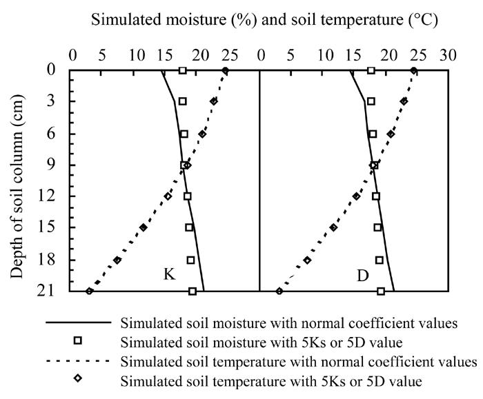
Simulated soil moisture and temperature distribution with saturation hydraulic conductivity of Ks and 5Ks (K) and soil moisture diffusivity of D and 5D (D), respectively, at initial soil water content of 18.5%, the upper and lower temperatures of 24.6 °C and 3.2 °C, respectively

(2) Sensitivity analysis of soil heat conductive coefficient

Sensitivity analysis of soil heat conductive coefficient was computed with changing soil porosity from 55.4% to 44.0% (Fig.5). The change of soil porosity had great impact on the change of soil thermal properties, resulting in the change of temperature, which would greatly influence moisture distribution.

Fig. 5.

Temperature distribution with soil porosity of 55.4% and 44.0%

CONCLUSION

1. For the closed column, the model of coupled soil moisture and heat transfer could predict well the spatial and temporal distributions of water and temperature, especially, those of temperature. But for the evaporating column, the simulation results for moisture contents did not agree very well with the measured results, so future improvement is needed.

2. Because the simulated thermal conductivity with empirical de Vries and Wierenga equations was less than the observed one, the predicted temperature did not accord with the observed one. So soil heat conductivity K _h should be corrected to fit the observed one. It is suggested that K _h, be modified by being multiplied by 8.0 at the first 6.5 h, and by 1.2 later.

3. The sensitivity of soil moisture transport coefficient was analyzed. Results indicated that the change of the unsaturated hydraulic conductivity K(θ) had a slight effect on moisture distribution in drier soils, and had significant effect for wetter soils. The changes of the moisture diffusivity D(θ) and soil moisture retention curve both had greater influence on moisture transport than on temperature distribution. Temperature distribution was more affected by the change of soil heat coefficients.

References

- 1.Bachmann J, Horton R, Ren T, Van der Ploeg RR. Comparison of the thermal properties of four wettable and four water-repellent soils. Soil Science Society American Proceedings. 2001;65:1675–1679. [Google Scholar]
- 2.Cai SY, Zhang YF. A numerical analysis of evaporation from soil under the effect of temperature. Journal of Hydraulic Engineering. 1991;11:1–8. (in Chinese) [Google Scholar]
- 3.Campbell GS. A simple method for determining unsaturated conductivity from moisture retention data. Soil Sci. 1974;117(6):311–314. [Google Scholar]
- 4.de Vries DA. Thermal Properties of Soils. In: van Wijk WR, editor. Physics of the Plant Environment. North-Holand, Amsterdam: 1963. [Google Scholar]
- 5.Genuchten V. A closed-form equation for predicting the hydraulic conductivity of unsaturated soils. Soil Science Society American Journal. 1980;44:892–898. [Google Scholar]
- 6.Gu ZY, Hong GS. Introduction and Application of Visual Basic. Beijing, China: Tsinghua University Press; 1996. (in Chinese) [Google Scholar]
- 7.Guan Y, Chen JL. Numerical Analysis. Beijing, China: Tsinghua University Press; 1990. (in Chinese) [Google Scholar]
- 8.Guo QR, Li YS. Mathematical simulation of heat and moisture coupling flow in soil under unsteady temperature. Journal of China Agricultural University. 1997;12(Suppl.):33–38. (in Chinese) [Google Scholar]
- 9.Han XF. Research on Coupled Soil Moisture and Heat Transport and Its Simulation Model. 1999. Dissertation of Master Degree of Huajia Campus, Zhejiang University, China (in Chinese) [Google Scholar]
- 10.Hu HP, Yang SX, Lei ZD. A numerical simulation for heat and moisture transfer during soil freezing. Journal of Hydraulic Engineering. 1992;7:1–8. (in Chinese) [Google Scholar]
- 11.Kang SZ, Liu XM, Gao XK, Xiong YZ. Computer simulation of moisture transport in SPAC (Soil-Plant-Atmosphere Continuum) Journal of Hydraulic Engineering. 1992;3:1–12. (in Chinese) [Google Scholar]
- 12.Kang SZ, Liu XM, Zhang GY. Simulation of soil water and heat movement with crop canopy shading. Journal of Hydraulic Engineering. 1993;3:11–17. 27. (in Chinese) [Google Scholar]
- 13.Kijune S, Corapcioglu MY, Malcolm CD. Heat and mass transfer in the vadose zone with plant roots. Journal of Contaminant Hydrology. 2002;57:99–127. doi: 10.1016/s0169-7722(01)00212-1. [DOI] [PubMed] [Google Scholar]
- 14.Lu J. Simulation of the effects of soil water condition on winter wheat growth. Journal of Hydraulic Engineering. 1998;7:68–72. (in Chinese) [Google Scholar]
- 15.Lu J, Huang ZZ, Han XF. Water and heat transport in hilly red soil of southern China: I. Experiment and analysis. J Zhejiang Univ SCI. 2005;6(5):331–337. doi: 10.1631/jzus.2005.B0331. [DOI] [PMC free article] [PubMed] [Google Scholar]
- 16.Mao XM, Yang SX, Lei ZD. Research on water and heat transfer in SPAC of winter wheat in Yerqiang irrigation area. Journal of Hydraulic Engineering. 1998;7:35–45. (in Chinese) [Google Scholar]
- 17.Philip JR, de Vries DA. Moisture movement in porous materials under temperature gradients. Transactions, American Geophysical Union. 1957;38:222–232. [Google Scholar]
- 18.Ren L, Zhang YF, Shen RK. Field experiments and numerical simulation of soil moisture and heat regimes under the condition of summer corn partially covered by mulch strips. Journal of Hydraulic Engineering. 1998;2:1–9. (in Chinese) [Google Scholar]
- 19.Sang SH, Lei ZD, Yang SX. Numerical simulation of soil moisture and thermal regime in winter. Irrigation and Drainage. 1997;16(3):12–17. (in Chinese) [Google Scholar]
- 20.Saxton KE, Rawls WJ, Romberger JS, Papendick RI. Estimating generalized soil-moisture characteristics from texture. Soil Science Society American Journal. 1986;50:1031–1036. [Google Scholar]
- 21.Shiozawa S, Campbell GS. On the calculation of mean particle diameter and standard deviation from sand, silt and clay fractions. Soil Science. 1991;152(6):427–431. [Google Scholar]
- 22.Taylor SA, Lary JW. Linear equations for the simultaneous flux of matter and energy in a continuous soil system. Soil Science Society American Journal. 1964;28:167–172. [Google Scholar]
- 23.Wierenga PJ, Nielson DR, Hagan RM. Thermal properties of a soil based upon field and laboratory measurements. Soil Science Society American Proceedings. 1969;3:354–360. [Google Scholar]
- 24.Yang BJ, Blackwell PS, Nicholson DF. Modeling heat and water movement in a water-repellent sandy soil. Acta Pedologica Sinica. 1996;33(4):351–359. (in Chinese) [Google Scholar]
- 25.Yang BJ, Sui HJ. Model and Application of Soil Moisture and Heat Movement. Beijing, China: Chinese Science and Technology Press; 1997. (in Chinese) [Google Scholar]
- 26.Yao XL. Soil Physics. Beijing, China: Agriculture Press; 1986. (in Chinese) [Google Scholar]