Feedback Functions, Optimization, and the Relation of Response Rate to Reinforcer Rate

Abstract

The present experiment arranged a series of inverted U-shaped feedback functions relating reinforcer rate to response rate to test whether responding was consistent with an optimization account or with a one-to-one relation of response rate to reinforcer rate such as linear system theory's rate equation or Herrnstein's hyperbola. Reinforcer rate was arranged according to a quadratic equation with a maximum at a unique response rate. The experiment consisted of two phases, during which 6 Long Evans rats lever pressed for food. In the first phase of the experiment, the rats responded on six fixed-interval-plus-quadratic-feedback schedules, and in the second phase the rats responded on three variable-interval-plus-quadratic-feedback schedules. Responding in both phases was inconsistent with a one-to-one relation of response rate to reinforcer rate. Instead, different response rates were obtained at equivalent reinforcer rates. Responding did vary directly with the vertex of the feedback function in both phases, a finding consistent with optimization of reinforcer rate. The present results suggest that the feedback function relating reinforcer rate to response rate imposed by a reinforcement schedule can be an important determinant of behavior. Furthermore, the present experiment illustrates the benefit of arranging feedback functions to investigate assumptions about the variables that control schedule performance.

Behavior can be conceptualized as the outcome of a feedback system wherein responding produces environmental changes that then affect responding, that then produces further environmental changes, and so on (Baum, 1973, 1981; McDowell & Wixted, 1986, 1988). Baum (1981) described an optimization account based on the concept of behavior as the outcome of a feedback system. According to Baum's optimization account, behavior is adjusted to maximize net gain, where net gain is defined as the benefits obtained from responding (e.g., reinforcer rate) minus the costs of responding (e.g., response effort). Baum concluded that this cost-benefit optimization account provided a better description of single-schedule variable-interval (VI) and variable-ratio (VR) performance than did the matching law (Herrnstein, 1970). More recent results from negative slope schedules, however, have been taken as strong evidence against optimization accounts of single-schedule performance (Jacobs & Hackenberg, 2000; Reed & Schachtman, 1989, 1991; Vaughan & Miller, 1984). On negative slope schedules, pigeons (Vaughan & Miller, 1984), rats (Reed & Schachtman, 1989, 1991), and humans (Jacobs & Hackenberg, 2000) typically respond at rates higher than necessary to maximize reinforcer rate, a finding inconsistent with optimization accounts that predict maximization of overall reinforcer rate.

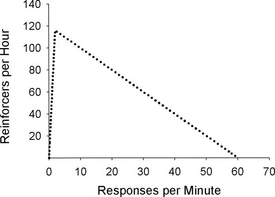
The use of negative slope schedules as tests of optimization derives from the feedback function relating reinforcer rate and response rate arranged by the schedules. Negative slope schedules arrange an inverted U-shaped relation of reinforcer rate to response rate. The dotted plot in Figure 1 illustrates the feedback function arranged by negative slope schedules. Negative slope schedules are constructed using linear VI schedules in combination with a fixed-ratio (FR) subtraction constraint. For response rates that are, on average, greater than 1 divided by the mean interreinforcer interval (IRI) of the linear VI schedule, reinforcer rate decreases linearly as response rate increases. Over the range of response rates less than 1 divided by the mean IRI, reinforcer rate is an increasing function of response rates. Thus negative slope schedules arrange a bitonic relation between reinforcer rate and response rate such that reinforcer rate first increases to a unique maximum and then decreases as a function of increasing response rate, providing a clear reference point for testing optimization accounts.

Fig 1. Reinforcer rate as a function of response rate on negative slope schedules.

An alternative to the optimization account of Baum (1981) that retains the notion of behavior as the outcome of a feedback system is an extension of the account provided by McDowell and Wixted (1986, 1988) for VR responding. According to McDowell and Wixted, stable state responding on VR schedules results from the interaction of two relations. One relation is the quantitative relation of response rate to reinforcer rate that is a property of the organism and the second is the quantitative relation of reinforcer rate to response rate imposed by the schedule of reinforcement. Specifically, McDowell and Wixted proposed that stable-state VR responding results from the interaction of linear system theory's rate equation (McDowell & Kessel, 1979) and the VR feedback function. The linear system theory rate equation can be written as:

1

where R represents response rate, r represents reinforcer rate, and m and b are parameters that must be estimated from fitting. Equation 1 states that response rate is an increasing, negatively accelerated function of reinforcer rate, given appropriate values of m and b.

The feedback function for VR schedules can be written as:

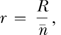2

where r and R are as defined previously and n ¯ represents the average response requirement. Equation 2 states that reinforcer rate is a linear function of response rate with slope 1/n ¯ and intercept 0.

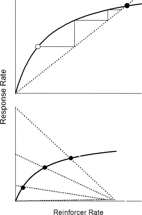
According to McDowell and Wixted (1988), an initial level of responding produces an initial reinforcer rate according to Equation 2, which then feeds back into Equation 1 to produce a new response rate, which then generates a new reinforcer rate according to Equation 2, and so on until responding stabilizes at the intersection of the two equations. This process is shown graphically in the top panel of Figure 2. Responding begins at the open circle and produces a reinforcer rate denoted by the horizontal line extending to the VR feedback function (dotted line), which produces a new response rate according to Equation 1 (solid curve) indicated by the vertical line, and so on until responding stabilizes at the level denoted by the filled circle.

Fig 2. Interaction of linear system theory rate equation and feedback functions on VR and negative slope schedules.

Top panel depicts the interaction of the rate equation (Equation 1; solid curve) and the VR feedback function (Equation 2; dotted line). Bottom panel depicts steady-state responding on three negative slope schedules.

The account described by McDowell and Wixted (1988) can be extended to any schedule of reinforcement for which the feedback function can be specified. For example, if an animal is exposed to a series of negative slope schedules, responding should stabilize at the intersection of the negative slope schedule feedback functions and Equation 1 as depicted in the bottom panel of Figure 2. Because the general form of Equation 1 is equivalent to Herrnstein's (1970) hyperbola, data from negative slope schedules that are consistent with Herrnstein's hyperbola are also consistent with McDowell and Wixted's account. Thus data such as those collected by Vaughan and Miller (1984), which those authors noted are consistent with Herrnstein's hyperbola, are also consistent with McDowell and Wixted's account.

One criticism of negative slope schedules as tests of optimization is that the apex of the feedback function typically occurs at very low response rates (e.g., for a negative slope schedule constructed using a linear VI 30-s schedule, the apex occurs at two responses per minute; see Figure 1). The present experiment sought to arrange a schedule using a bitonic feedback function that avoided this criticism of negative slope schedules. It arranged an inverted U-shaped feedback function for which the response rate at which reinforcer rate was maximized could be varied over a wide range. Additionally, the feedback function was chosen such that all positive response rates produced a positive reinforcer rate; a feature common to typical schedules such as VI and VR but different from negative slope schedules.

Feedback was arranged in the present experiment using the following equation:

3

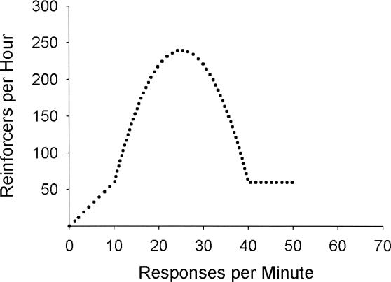
where r represents reinforcers per hour, R represents response per minute, and a, b, c, p₀, and p₁ are experimenter-chosen parameters. The dotted curve in Figure 3 depicts the relation described by Equation 3. Equation 3 is a piecewise-defined function where for response rates less than p₀, the operative equation is a straight line of slope with intercept zero. This portion of the function is necessary to ensure that the function intersects the origin. For response rates between p₀ and p₁, the operative equation is a quadratic equation with parameters a, b, and c. Finally, for response rates greater than or equal to p₁, the operative equation is a horizontal line equal to . The third portion of Equation 3 was chosen to ensure that all positive response rates produce a positive reinforcer rate.

Fig 3. Reinforcer rate as a function of response rate according to Equation 3.

In the first phase of the experiment, feedback was arranged by adjusting a fixed-interval (FI) schedule according to Equation 3 (a FI-plus-quadratic-feedback or FI+QF schedule). In the second phase of the experiment, feedback was arranged by adjusting the mean of a VI schedule according to Equation 3 (a VI-plus-quadratic-feedback or VI+QF schedule). Both FI and VI schedules were used to determine if differences in IRI variability between the two schedules would affect the pattern of response rates obtained. In either case, the main question concerned the pattern of response rates across schedules.

One possible outcome is for response rates to be consistent with a one-to-one relation of response rate to reinforcer rate such as Herrnstein's (1970) hyperbola or linear system theory's rate equation (Equation 1). In contrast, strict optimization of overall reinforcer rate predicts that responding should equal the vertex of Equation 3. Alternatively, Baum's (1981) cost-benefit optimization account predicts that subjects should maximize net gain, which in the present experiment is equivalent to maximizing overall reinforcer rate given a constraint on maximal response rate. Thus Baum's account predicts that responding should vary with the vertex of Equation 3 but should deviate from the vertex at high vertex rates (i.e., as the cost of responding becomes substantial).

Method

Subjects

Six Long Evans hooded rats, approximately 6 months old at the start of the experiment and maintained at 85% of free-feeding weight, served as subjects. Rats were fed following each daily session. Rats were housed individually in a colony room illuminated 12 hr daily from 8:00 a.m. until 8:00 p.m. Access to water was unrestricted in the home cages.

Apparatus

The experimental chambers were six standard, two response lever operant chambers (Med Associates, Inc. ENV-007), 240 mm wide, 305 mm deep, and 290 mm high. Each chamber was housed in a sound-attenuating cubicle. The response levers were positioned on the front panel of the chamber 70 mm above the floor and were separated by 115 mm. Each lever required a force of approximately 0.68 N to register a response. A food receptacle measuring 50 mm by 50 mm by 30 mm was located equidistant between the two response levers. Three stimulus lights, 8 mm in diameter, were arranged 70 mm above each response lever. The light colors from left to right were red, yellow, and green. Each chamber was equipped with a ventilation fan that along with an external white noise generator masked extraneous sounds. A 28-V DC houselight was centered on the back panel of the chamber 20 mm from the ceiling.

Procedure

Sessions were conducted 7 days per week in the mornings. Rats initially were trained to lever press through exposure to an FR 1 schedule for eight sessions. Following FR 1 exposure, the ratio was increased to 2 for two sessions. Following FR 2 exposure, rats were exposed to VI 4, 10, and 20 s for 1, 4, and 20 sessions, respectively. Finally, rats were exposed to VR 4 and then VR 8 for 10 and 7 sessions, respectively. Following VR 8 exposure, the first phase of the experiment began.

In the first phase, rats were exposed to six FI+QF schedules: Feedback was arranged according to Equation 3 in the following manner: Each time a response occurred, the response rate since the previous reinforcer or since the beginning of the session if no reinforcers had been delivered, was calculated. A scheduled IRI was then calculated by first calculating reinforcer rate according to Equation 3 and then taking its reciprocal. If the time elapsed since the previous reinforcer, or the start of the session if no reinforcers had been delivered, was equal to or longer than the scheduled IRI, a reinforcer was delivered. Otherwise, the calculations repeated with the next response. Reinforcers consisted of deliveries of 45-mg sucrose pellet (NOYES, Formula P). Sessions were terminated after 60 reinforcers or 60 min, whichever occurred first.

In the second phase of the experiment, rats were exposed to three VI+QF schedules. Fleshler and Hoffman's (1962) equation for generating individual IRIs was used in combination with Equation 3 to generate the VI+QF schedules. Fleshler and Hoffman's equation can be written as:

4

where N is the number of IRIs, i is an integer between 1 and N, and is the mean IRI. Feedback was arranged according to Equation 3 in the following manner: At the beginning of each session and following each reinforcer, i in Equation 4 was randomly set to an integer value between 1 and 20. Each time a response occurred, the response rate was calculated as in the first phase of the experiment, and a calculated reinforcer rate was generated from Equation 3. The reciprocal of the calculated reinforcer rate, the calculated , then was used to generate 20 intervals according to Equation 4. The chosen index value, i, then was used to select a particular IRI from the 20 generated intervals. If the time elapsed from the previous reinforcer, or start of the session if no reinforcers had been delivered, was longer than or equal to the selected IRI, a reinforcer was delivered. Otherwise, the calculations began anew with the next response.

Table 1 lists the schedule parameters employed in both phases of the experiment. The values of a, b, c, p₀, and p₁ in Equation 3 are given along with the name used to describe the schedule in the text. The naming convention designates the schedule type (FI+QF or VI+QF) followed by the vertex and the maximum obtainable reinforcer rate in parentheses. For example, FI+QF (25, 240) designates the FI-plus-quadratic-feedback schedule for which the vertex of the equation occurred at 25 responses per minute and the peak reinforcer rate at that response rate was 240 reinforcers per hour. Rats 151, 152, and 153 were exposed to the schedules in the following order: FI+QF (25, 240), FI+QF (37.5, 240), FI+QF (50, 240), FI+QF (50, 156), FI+QF (37.5, 156), FI+QF (25, 156), VI+QF (25, 240), VI+QF (37.5, 240), and VI+QF (50, 240). Rats 154, 155, and 156 were exposed to the schedules in the following order: FI+QF (50, 240), FI+QF (37.5, 240), FI+QF (25, 240), FI+QF (25, 156), FI+QF (37.5, 156), FI+QF (50, 156), VI+QF (50, 240), VI+QF (37.5, 240), and VI+QF (25, 240).

Table 1. Parameters of Equation 3 used for each schedule. Schedules are named by designating the type (FI+QF or VI+QF) followed by the response-rate vertex of the function (responses per minute) and the maximum obtainable reinforcers per hour in parentheses.

Schedule	a	b	c	p0	p1
FI+QF (25, 240)	0.8	40	260	10	40
FI+QF (37.5, 240)	0.8	60	885	22.5	52.5
FI+QF (50, 240)	0.8	80	1,760	35	65
FI+QF (25, 156)	0.25	12.5	0.25	5.4	44.6
FI+QF (37.5, 156)	0.25	18.75	195.6	17.9	57.1
FI+QF (50, 156)	0.25	25	469	30.4	69.6
VI+QF (25, 240)	0.8	40	260	10	40
VI+QF (37.5, 240)	0.8	60	885	22.5	52.5
VI+QF (50, 240)	0.8	80	1,760	35	65

Rats were exposed to each schedule until a seven-session block of responding met the following criteria: the average within-IRI response rate (response rate calculated only from responses and time occurring between two reinforcers or between the start of the session and the first reinforcer delivery) of the first three sessions and the last three sessions in the seven-session block differed by no more than 20%, the average within-IRI response rate of the first three sessions and the last three sessions in the seven-session block differed from the average of the seven sessions by no more than 10%, and no visible trends were evident over the seven-session block.

Results

Table 2 presents the number of sessions at which stability was achieved on each schedule for each rat. The number of sessions required to achieve stability varied between 7 and 31. The median number of sessions required to achieve stability was 13.

Table 2. Number of sessions required for stability. The response-rate vertex of the function (responses per minute) and the maximum obtainable reinforcers per hour are in parentheses.

Schedule	Rat
	151	152	153	154	155	156
FI+QF (25, 240)	31	31	28	11	22	9
FI+QF (37.5, 240)	12	19	13	13	13	12
FI+QF (50, 240)	9	16	11	28	29	29
FI+QF (25, 156)	10	14	20	23	18	14
FI+QF (37.5, 156)	14	16	13	14	12	19
FI+QF (50, 156)	17	30	23	18	11	20
VI+QF (25, 240)	12	7	15	7	7	8
VI+QF (37.5, 240)	9	11	7	9	10	9
VI+QF (50, 240)	12	8	7	7	10	10

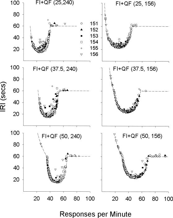
Because the schedules employed are unfamiliar, it is instructive to understand how the feedback arranged by Equation 3 actually worked from IRI to IRI. Figure 4 plots the obtained IRI preceding each reinforcer as a function of the response rate during the IRI for each FI+QF schedule. Each panel depicts IRIs for all 6 rats from the last session of stable responding for each schedule. Figure 4 illustrates that obtained IRIs were governed by the reciprocal of Equation 3, which is plotted as a dashed line in each panel. Some IRIs fall above the dashed line, consistent with the requirement that the elapsed time at the reinforced response equal or exceed the scheduled IRI.

Fig 4. IRI as a function of within-IRI response rate for FI+QF schedules.

Each panel depicts data from an individual schedule. The dashed line represents the reciprocal of Equation 3.

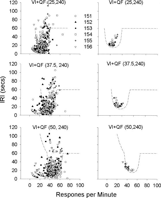
The left column of Figure 5 depicts obtained IRI preceding each reinforcer as a function of response rate during the IRI in the last session of exposure to the VI+QF schedules. The right column of Figure 5 depicts average IRI obtained from each session of stable responding as a function of average within-IRI response rate for the VI+QF schedules. The left column of graphs shows that more variability occurred in obtained IRIs on the VI+QF schedules than on the FI+QF schedules (see Figure 4), as to be expected. The right column of graphs shows that at the session level, average IRI falls closer to the feedback function than do individual IRIs.

Fig 5. IRI as a function of within-IRI response rate for VI+QF schedules.

Each panel depicts data from an individual schedule. The dashed line in each panel represents the reciprocal of Equation 3. The left column depicts the obtained IRI preceding each reinforcer from the last session of stable responding for each rat. The right column depicts the average IRI obtained from each session of stable responding for each rat.

Table 3 shows obtained reinforcer rates and within-IRI response rates. One noteworthy feature of Table 3 is the difference in response rates obtained on the different schedules despite relatively equivalent reinforcer rates. A two-factor repeated measures analysis of variance (ANOVA) was conducted on response rates using schedule as a within-subjects factor and group as a between-subjects factor. The ANOVA revealed a main effect of schedule, F(8, 32)  =  58.07, p < 0.05, no significant effect of group, F(1, 4)  =  0.97, p > 0.05, and a significant interaction of schedule and group, F(8, 32)  =  23.29, p < 0.05. A post hoc Tukey analysis revealed a significant difference between the mean response rates of the two groups on the FI+QF (37.5, 156) and FI+QF (50, 156) schedules. All remaining comparisons were not significant. Thus the ANOVA revealed a possible effect of order of schedule presentation on responding for the FI+QF (37.5, 156) and FI+QF (50, 156) schedules.

Table 3. Reinforcers per hour, responses per minute, and standard deviation (SD) of responses per minute on each schedule.

Rat	Schedule	Reinforcers per hour	Responses per minute (SD)
151	FI+QF (25, 240)	152.75	27.61 (7.52)
	FI+QF (37.5, 240)	152.75	36.01 (7.98)
	FI+QF (50, 240)	155.75	46.69 (7.24)
	FI+QF (25, 156)	117.54	29.07 (9.05)
	FI+QF (37.5, 156)	115.84	37.95 (10.80)
	FI+QF (50, 156)	105.19	50.32 (12.65)
	VI+QF (25, 240)	155.85	25.13 (8.57)
	VI+QF (37.5, 240)	163.42	37.98 (9.26)
	VI+QF (50, 240)	171.94	49.87 (9.29)
152	FI+QF (25, 240)	164.32	24.48 (7.25)
	FI+QF (37.5, 240)	162.93	35.62 (7.57)
	FI+QF (50, 240)	150.22	45.35 (7.75)
	FI+QF (25, 156)	132.84	24.09 (6.06)
	FI+QF (37.5, 156)	123.64	35.83 (8.99)
	FI+QF (50, 156)	104.11	44.90 (12.24)
	VI+QF (25, 240)	163.69	19.48 (7.85)
	VI+QF (37.5, 240)	136.50	28.99 (10.39)
	VI+QF (50, 240)	135.59	39.55 (12.88)
153	FI+QF (25, 240)	167.68	21.75 (5.57)
	FI+QF (37.5, 240)	159.72	31.95 (5.82)
	FI+QF (50, 240)	151.39	43.23 (6.21)
	FI+QF (25, 156)	133.57	23.43 (6.27)
	FI+QF (37.5, 156)	129.35	33.70 (7.50)
	FI+QF (50, 156)	111.33	41.88 (7.50)
	VI+QF (25, 240)	178.65	23.66 (7.13)
	VI+QF (37.5, 240)	161.58	31.87 (7.39)
	VI+QF (50, 240)	130.82	39.46 (9.78)
154	FI+QF (25, 240)	139.27	26.11 (9.00)
	FI+QF (37.5, 240)	145.92	37.60 (9.12)
	FI+QF (50, 240)	141.21	49.90 (9.47)
	FI+QF (25, 156)	114.62	22.98 (9.70)
	FI+QF (37.5, 156)	119.67	32.22 (8.75)
	FI+QF (50, 156)	49.98	38.14 (10.95)
	VI+QF (25, 240)	126.43	23.75 (10.18)
	VI+QF (37.5, 240)	135.97	33.43 (11.00)
	VI+QF (50, 240)	138.60	39.06 (13.74)
155	FI+QF (25, 240)	136.23	24.78 (9.46)
	FI+QF (37.5, 240)	132.10	37.98 (10.80)
	FI+QF (50, 240)	99.04	44.40 (11.94)
	FI+QF (25, 156)	120.21	25.17 (9.21)
	FI+QF (37.5, 156)	111.40	29.34 (7.90)
	FI+QF (50, 156)	56.78	32.63 (7.86)
	VI+QF (25, 240)	106.53	29.55 (10.43)
	VI+QF (37.5, 240)	147.28	38.45 (10.01)
	VI+QF (50, 240)	146.74	42.12 (12.69)
156	FI+QF (25, 240)	159.75	19.95 (5.61)
	FI+QF (37.5, 240)	133.72	28.64 (4.19)
	FI+QF (50, 240)	69.46	38.56 (5.40)
	FI+QF (25, 156)	108.97	15.49 (5.83)
	FI+QF (37.5, 156)	66.52	24.81 (8.55)
	FI+QF (50, 156)	47.68	37.89 (9.61)
	VI+QF (25, 240)	159.35	22.09 (7.10)
	VI+QF (37.5, 240)	137.55	31.31 (9.62)
	VI+QF (50, 240)	101.30	39.74 (11.29)

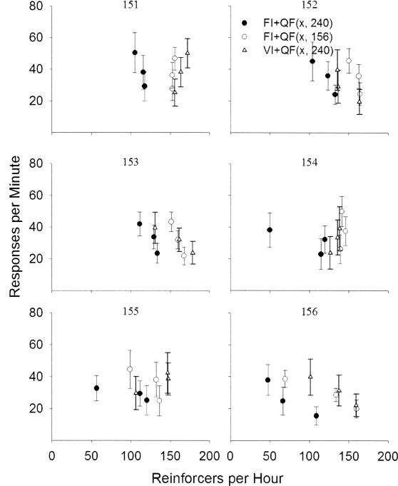
Figure 6 depicts average within-IRI response rate as function of average reinforcer rate. Each panel depicts data for an individual rat. One noteworthy feature of Figure 6 is that response rates do not appear to be systematically related to reinforcer rate.

Fig 6. Response rate as a function of reinforcer rate.

Each panel represents data for an individual rat. Open and filled circles represent data from FI+QF (x, 156) and FI+QF (x, 240) schedules, respectively, where x was 25, 37.5, or 50 responses per minute, and open triangles represent data from VI+QF schedules. Error bars represent plus or minus one standard deviation.

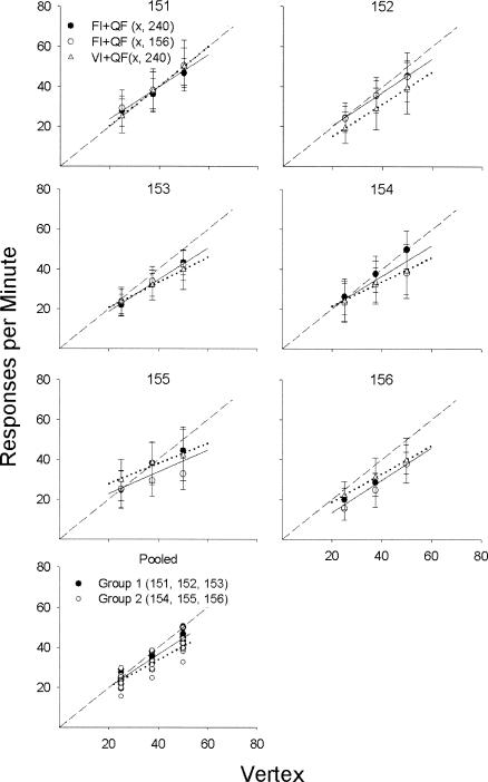
Figure 7 depicts average within-IRI response rates as a function of the vertex of Equation 3, b/(2a). The top six panels each depict data for an individual rat. Regression lines were fitted to the FI+QF data and VI+QF data separately. The slope and intercept of the best-fitting regression line and the obtained percentage of variance accounted for (%VAC) are listed in Table 4. Overall, responding was well described by a straight line. For the FI+QF schedules, the average %VAC by the regression equation was 89.07 with a high of 99.63 and a low of 62.19. For the VI+QF schedules, the average %VAC by a straight line was 98.58 with a high of 99.93 and a low of 96.32.

Fig 7. Response rate as a function of the vertex of Equation 3.

Each of the upper six panels represents data for an individual rat. Open and filled circles represent data from FI+QF (x, 156) and FI+QF (x, 240) schedules, respectively, where x was 25, 37.5, or 50 responses per minute, and open triangles represent data from VI+QF schedules. Error bars represent plus or minus one standard deviation. The solid line in each panel represents the best-fitting regression equation for the FI+QF schedules. The dotted line in each panel represents the best-fitting regression equation for the VI+QF schedules. The bottom panel shows the data pooled across the 6 rats. The solid regression line is for Rats 151, 152, and 153; the dotted line is for Rats 154, 155, and 156.

Table 4. Slope (m), intercept (b), and percentage of variance accounted for (%VAC) by a straight line fitted to the response rate versus vertex data.

Rat	FI+QF schedules			VI+QF schedules
	m	b	%VAC	m	b	%VAC
151	0.81	7.70	97.06	0.99	0.56	99.95
152	0.83	3.78	99.63	0.80	−0.76	99.91
153	0.80	2.71	99.02	0.63	7.96	99.95
154	0.78	5.28	80.98	0.61	9.11	97.73
155	0.54	12.07	62.19	0.50	17.85	94.55
156	0.82	−3.20	95.55	0.71	4.58	99.93

The bottom panel of Figure 7 depicts pooled data for all rats. Response rates are plotted separately for each group of rats. Regression equations were fitted to the data for the two groups of rats separately. The solid and dotted lines represent the best-fitting regression equations for Group 1 (151, 152, and 153) and 2 (154, 155, and 156), respectively. The slopes and intercepts of the regression equations were 0.81 and 4.02 for Group 1 and 0.68 and 6.65 for Group 2. The best-fitting regression equations diverge for the two groups as the vertex increases, which is consistent with the ANOVA results indicating a significant difference between the two groups' response rates on the FI+QF (37.5, 156) and FI+QF (50, 156) schedules. Still, the general pattern is the same: the slopes of the regression equations are positive and less than 1.0, and the y-intercepts are positive.

Discussion

The main finding of the present experiment was that response rate varied directly with the vertex of Equation 3 (see Figure 7). Response rate versus the feedback function vertex data were well described by a straight line, which in most cases had a slope less than 1.0 and a positive y-intercept (exceptions were 156 for the FI+QF schedules and 152 for the VI+QF schedules). Although order of schedule presentation may have affected absolute response rates on the FI+QF (37.5, 156) and FI+QF (50, 156) schedules (see bottom panel of Figure 7), the general pattern of response rates was the same for both groups of rats. Additionally, response rate versus reinforcer rate data were not consistent with a one-to-one relation of response rate to reinforcer rate as evidenced by differences in response rate obtained at equivalent reinforcer rates (see Table 3 and Figure 6).

The results from the FI+QF and VI+QF schedules did not differ substantially. The relation between response rate and the vertex of Equation 3 was linear for both schedule types, although the slopes of the regression equations from the VI+QF fits tended to be lower than those obtained from the FI+QF fits. This may have been due to differences in the discriminability of the relation between reinforcer rate and response rate on the two schedule types. This possibility seems unlikely, however, because a decrease in discriminability presumably would result in a greater number of sessions required to reach stability, yet the median number of sessions required for stability on the FI+QF schedules (16) was higher than on the VI+QF schedules (9). Thus further research is necessary to determine if the difference between FI+QF and VI+QF schedules can be replicated and if so, to determine the variables responsible for the difference.

One issue of interest is why rats in the present experiment tended to respond at the vertex of the feedback function whereas subjects in experiments on negative slope schedules respond at rates much higher than the vertex of the feedback function (Jacobs & Hackenberg, 2000; Reed & Schachtman, 1989, 1991; Vaughan & Miller, 1984). One possibility is the difference in the vertex of the feedback function in the present experiment and in negative slope schedule experiments. In the present experiment, the response rates at which reinforcer rate was maximized were higher (25 to 50 responses per minute) than in negative slope schedule experiments (typically less than or equal to two responses per minute). The finding of slopes less than 1.0 and positive y-intercepts of the regression equation relating response rate and the vertex of Equation 3 might explain the difference in results. This is because the finding of slopes less than 1.0 and positive y-intercepts suggests that as the vertex of the function decreases, response rate will increasingly exceed that vertex. Of course, this assumes that the straight-line relation holds at lower vertex values, a suggestion requiring experimental confirmation. Future research can inform this suggestion by arranging FI+QF and VI+QF schedules for which the apex occurs at a very low response rate, as on negative slope schedules.

Another question of interest is why, in the present experiment, it appears that rats were sensitive to the molar relation between reinforcer rate and response rate, but in experiments where linear feedback has been added to VI schedules (VI+LF schedules), some researchers have concluded that subjects were not sensitive to the arranged feedback function (Cole, 1999; Reed, Hildebrandt, DeJongh, & Soh, 2003; Reed, Soh, Hildebrandt, DeJongh, & Shek, 2000). An explanation is not readily available, and differences in design make comparison difficult. Two of the studies noted (Reed et al., 2003; Reed et al., 2000) did not vary the parameters of the arranged feedback function; rather, comparisons were made between a single VI+LF schedule and a yoked VI schedule. If responding on the VI+LF schedule was different from responding on the yoked VI schedule but not optimal, the authors concluded that subjects were not sensitive to the feedback arranged by the VI+LF schedule, the presumption being that if differences in responding reflected sensitivity to the feedback function, then responding should be optimal. Therefore, the authors concluded that some other factor, such as interresponse time (IRT) reinforcement, must be responsible for the differences in responding. This argument assumes, however, that sensitivity will produce optimal responding, an assumption that may or may not be correct.

An alternative approach to assessing sensitivity to the feedback function is to arrange a series of VI+LF schedules and examine whether response rate varies systematically with the feedback function parameters. A finding of systematic variation in response rate would support the conclusion that subjects are sensitive to the feedback arranged by the VI+LF schedules. The studies by Cole (1999) and McDowell and Wixted (1986) provided data of this kind. In both studies, response rate varied with the parameters of the arranged feedback function, suggesting some degree of sensitivity to the feedback function. Such data do not rule out the possibility of IRT reinforcement, however, because without explicit controls, response rate and reinforced IRT measures typically will be confounded.

Although speculative, another possibility that may explain the sensitivity to the molar relation between reinforcer and response rate in the present experiment is that the present schedules may partially mimic contingencies in the natural environment. One property of the current schedules is that too low or high of a response rate produces a low reinforcer rate. Consider the analogy of visiting a feeding patch in the wild. Infrequent visits to the patch fail to produce significant gains. Overly frequent visits may deplete the patch and reduce overall gains. The feedback function employed in the present experiment partially captures this aspect of patch visiting. One important difference, however, is the third portion of the feedback function, which arranges a constant reinforcer rate for response rates greater than p₁. This feature has no obvious counterpart in natural environments. Still, if the analogy is accurate for the bitonic portion of the feedback function, FI+QF and VI+QF schedules might capture an important aspect of the natural environment, and animals, therefore, might be particularly well suited to maximize reinforcer rate on such schedules.

The present results demonstrate that under some conditions, rats can respond at rates that produce the maximum obtainable reinforcer rate and that the feedback function relating reinforcer rate and response rate can be an important determinant of behavior. Although the variation in response rates across schedules is incompatible with accounts that specify a one-to-one relation between response rate and reinforcer rate (e.g., linear system theory and Herrnstein's hyperbola), the pattern of response rates across schedules generally is consistent with Baum's (1981) cost-benefit optimization account. The finding that response rates tended to fall beneath the optimal rate as the vertex of Equation 3 increased (see Figure 7) is consistent with the prediction of Baum's account that responding should maximize overall reinforcer rate given a constraint on maximal response rate, especially given the relatively high response cost required for lever pressing (0.68 N).

The finding that the y-intercepts of the regression equations relating response rate to the vertex of Equation 3 usually were greater than 0 suggests that as the vertex is decreased, responding will increasingly exceed the optimal rate. This suggestion, if confirmed, would be inconsistent with Baum's account. It is important to note, however, that in the present experiment, response rates rarely exceeded the vertex even at the lowest vertex values. Still, if this prediction was confirmed, Baum's account might easily be modified to incorporate a limit on how slowly subjects can respond. Such a limit is supported by data suggesting that, at least on VI schedules, low response rates may be associated with response bursting (Baum, 1992).

The present experiment provides an example of how the use of feedback functions can illuminate schedule performance. The methods employed here can be used to arrange virtually any relation between reinforcer rate and response rate. Furthermore, the approach need not be restricted to interval schedules. For example, the mean ratio of a VR schedule might be adjusted based on response rate. In fact, any property of the environment under experimenter control can be adjusted based on any measured property of behavior. Of course, the properties for which an experimenter chooses to arrange a feedback relation will say something about the variables the experimenter assumes control behavior (Baum, 1973). In any case, the use of feedback functions to arrange new and interesting environments can test our assumptions about the variables that control behavior and should therefore improve our understanding of behavior.

References

- Baum W.M. The correlation-based Law of Effect. Journal of the Experimental Analysis of Behavior. 1973;20:137–153. doi: 10.1901/jeab.1973.20-137. [DOI] [PMC free article] [PubMed] [Google Scholar]
- Baum W.M. Optimization and the matching law as accounts of instrumental behavior. Journal of the Experimental Analysis of Behavior. 1981;36:387–403. doi: 10.1901/jeab.1981.36-387. [DOI] [PMC free article] [PubMed] [Google Scholar]
- Baum W.M. In search of the feedback function for variable-interval schedules. Journal of the Experimental Analysis of Behavior. 1992;57:365–375. doi: 10.1901/jeab.1992.57-365. [DOI] [PMC free article] [PubMed] [Google Scholar]
- Cole M.R. Molar and molecular control in variable-interval and variable-ratio schedules. Journal of the Experimental Analysis of Behavior. 1999;71:319–328. doi: 10.1901/jeab.1999.71-319. [DOI] [PMC free article] [PubMed] [Google Scholar]
- Fleshler M, Hoffman H.S. A progression for generating variable-interval schedules. Journal of the Experimental Analysis of Behavior. 1962;5:529–530. doi: 10.1901/jeab.1962.5-529. [DOI] [PMC free article] [PubMed] [Google Scholar]
- Herrnstein R.J. On the law of effect. Journal of the Experimental Analysis of Behavior. 1970;13:243–266. doi: 10.1901/jeab.1970.13-243. [DOI] [PMC free article] [PubMed] [Google Scholar]
- Jacobs E.A, Hackenberg T.D. Human performance on negative slope schedules of points exchangeable for money: A failure of molar maximization. Journal of the Experimental Analysis of Behavior. 2000;73:241–260. doi: 10.1901/jeab.2000.73-241. [DOI] [PMC free article] [PubMed] [Google Scholar]
- McDowell J.J, Kessel R. A multivariate rate equation for variable-interval performance. Journal of the Experimental Analysis of Behavior. 1979;31:267–283. doi: 10.1901/jeab.1979.31-267. [DOI] [PMC free article] [PubMed] [Google Scholar]
- McDowell J.J, Wixted J.T. Variable-ratio schedules as variable-interval schedules with linear feedback loops. Journal of the Experimental Analysis of Behavior. 1986;46:315–329. doi: 10.1901/jeab.1986.46-315. [DOI] [PMC free article] [PubMed] [Google Scholar]
- McDowell J.J, Wixted J.T. The linear system theory's account of behavior maintained by variable-ratio schedules. Journal of the Experimental Analysis of Behavior. 1988;49:143–169. doi: 10.1901/jeab.1988.49-143. [DOI] [PMC free article] [PubMed] [Google Scholar]
- Reed P, Hildebrandt T, DeJongh J, Soh M. Rats' performance on variable-interval schedules with a linear feedback loop between response rate and reinforcement rate. Journal of the Experimental Analysis of Behavior. 2003;79:157–173. doi: 10.1901/jeab.2003.79-157. [DOI] [PMC free article] [PubMed] [Google Scholar]
- Reed P, Schachtman T.R. Instrumental responding by rats on free operant contingencies with componenents that schedule response-dependent reinforcer omission. Animal Learning and Behavior. 1989;17:328–338. [Google Scholar]
- Reed P, Schachtman T.R. Instrumental performance on negative schedules. The Quarterly Journal of Experimental Psychology. 1991;43B:177–197. [Google Scholar]
- Reed P, Soh M, Hildebrandt T, DeJongh J, Shek W.Y. Free-operant performance on variable interval schedules with a linear feedback loop: No evidence for molar sensitivities in rats. Journal of Experimental Psychology: Animal Behavior Processes. 2000;26:416–427. doi: 10.1037//0097-7403.26.4.416. [DOI] [PubMed] [Google Scholar]
- Vaughan W, Jr, Miller H.L., Jr Optimization versus response-strength accounts of behavior. Journal of the Experimental Analysis of Behavior. 1984;42:337–348. doi: 10.1901/jeab.1984.42-337. [DOI] [PMC free article] [PubMed] [Google Scholar]