A method for evaluating the structural quality of protein models by using higher-order φ–ψ pairs scoring

Abstract

A method is presented for scoring the model quality of experimental and theoretical protein structures. The structural model to be evaluated is dissected into small fragments via a sliding window, where each fragment is represented by a vector of multiple φ–ψ angles. The sliding window ranges in size from a length of 1–10 φ–ψ pairs (3–12 residues). In this method, the conformation of each fragment is scored based on the fit of multiple φ–ψ angles of the fragment to a database of multiple φ–ψ angles from high-resolution x-ray crystal structures. We show that measuring the fit of predicted structural models to the allowed conformational space of longer fragments is a significant discriminator for model quality. Reasonable models have higher-order φ–ψ score fit values (m) > −1.00.

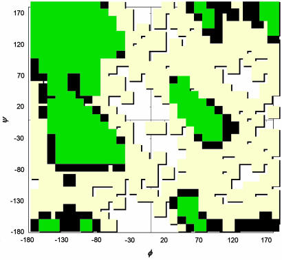
The typical end scenario for those who try to predict protein structure by theoretical means (ab initio) or for crystallographers with poorly resolved data is a model for which there are no assessment methods at present for the quality of the model. Assessment can only occur, post facto, after the high-quality experimental structures become available. One of the earliest methods for determining structural quality was implemented in the suite of utilities distributed as procheck by the Thornton laboratory (1, 2). The G-factor, a measure of fit to the most frequently occupied regions of φ–ψ space (Fig. 1), and the φ–ψ plot itself became tools of the crystallographer for standardizing the quality of the model as a whole and troublesome portions of the structure (perhaps a coil region with poorly resolved electron density). In a more recent study, Shortle (3, 4) used a scoring function with finer subdivisions of the φ–ψ plot (and sequence-specific probabilities assigned to each subdivision) to distinguish between native and non-native decoys.

Fig. 1.

Ramachandran φ–ψ plot. Regions of the φ–ψ space are divided into “core” favorable regions (green), allowed regions (blue), unfavored regions (tan), and disallowed regions (white). Overall, the plot shows four conformational clusters with their centers around the (φ,ψ) values of (−100, −30), (−100, 120), (60, 0), and (60, 180) degrees.

Unfortunately, the G-factor and the simple φ–ψ plot cannot, in most cases, be used as tools to evaluate the quality of a theoretical structure, because information from the φ–ψ plot itself (in the form of minimum contact distances and torsion angle force constants) is used as a constraint in the refinement and minimization processes. Thus, a predicted structure may fit the constraints of the φ–ψ plot exceedingly well at the single-residue level, yet be composed of very unnatural building blocks consisting of multiple residues, as opposed to the commonly observed fragments of structure we see in high-resolution experimental structures.

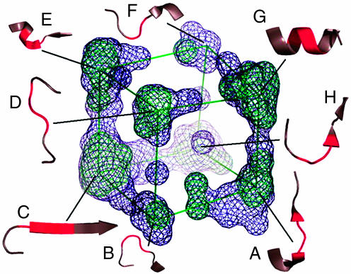
In our previous work (5), we investigated the angular conformational spaces of longer peptide fragments, fragments >3 residues in length with multiple φ–ψ angle pairs. Because each fragment was represented by its torsion angles, the length of the fragment is represented by the number of φ–ψ angle pairs. We used a multivariate analysis method called multidimensional scaling to reduce multiangle spaces to 3D conformational maps to extract and visualize the major features of the multidimensional φ–ψ angle space, the higher-order φ–ψ (HOPP) maps. An example for the peptides with three pairs of φ–ψ angles is given in Fig. 2. What we observed is that there were defined regions of space representing discrete conformations or common building blocks, and the number of conformational clusters, y, is related to the number of φ–ψ pairs, k, via the simple relationship,

Fig. 2.

3D map of conformational space for the peptides with three φ–ψ values and representative conformations. To extract and visualize the major features of a HOPP map, the highest three eigen values of the HOPP space are plotted in this map. The multidimensional scaling projections are represented as wire mesh surfaces at two colored contour (σ) levels into a medium- and high-density region (blue, 2σ; green, 3σ). Each conformation (in red) is indicated in the context of the local structure in which the sample conformation was found in crystal structures. Annotated conformations are as follows: A, turn type II; B, turn type II; C, β-extended; D, turn type I; E, helical N-cap; F, turn type II; G, helix; H, turn type I. For more information see ref. 5.

which compares well with other estimates by Dill (6) and Tendulkar et al. (7), but dramatically smaller than estimates implied by Levinthal (8) (y = 9^k; three possible φ values × three possible ψ values for each φ–ψ pair) or Ramachandran and Sasisekharan (9) (y = 4^k; four observed conformational clusters for each φ–ψ pair as shown in Fig. 1). Thus, the size of accessible conformational space is significantly reduced by steric hindrances that extend beyond nearest-chain residues (10). This observation suggests that: (i) protein structure might best be represented as blocks of fragments with designated accessible φ–ψ values, and (ii) it may be possible to construct and delineate a conformational space into a finite number of conformational clusters for a given number of φ–ψ pairs.

In this work we present a method, HOPPscore, for defining the conformational space of multiple φ–ψ pairs and testing the fit of queried protein structural models to each of those conformational spaces. We show the relationship between model resolution and HOPPscore and how HOPPscore can be used to assess the overall quality of theoretical structural models, e.g., from the Critical Assessment of Protein Structure Prediction (CASP) contests (11), or identify the local quality of less reliable regions of an experimental structural model.

Results and Discussion

Construction of the HOPPscore Database.

Conformational hash tables.

Our first task was to collect a data set of nonredundant (<25% sequence identity) x-ray crystal structures from the October 2004 PDBselect Database (12). We then divided the database into bins by resolution in 0.2-Å intervals from 0.5 to 3.0 Å (The actual resolution of the structures ranges from 0.54 to 2.9 Å.) We then created reference hash table databases of multiple φ–ψ angles for a given peptide length for each resolution threshold (i.e., the 1.6-Å resolution level contains all structures from 0.54 to 1.6 Å inclusively). These hash tables form a conformational reference database or “lookup table” used for scoring the quality of query structures within the HOPPscore. The backbone φ–ψ angles for each structure were calculated by using dssp (13), and fragments were extracted by using windows of size k = 1–10 φ–ψ pairs, creating vectors of multiple φ and ψ angles describing each fragment. For each resolution threshold level, window size (k), and grid size (the coarseness by which the φ–ψ space is divided) we created a lookup table. The lookup or hash table contains the frequency for which a particular conformation appears within the database. For further information regarding the method of constructing the hash tables see Materials and Methods.

CASP model database.

All of the CASP models were collected from the CASP web site (http://predictioncenter.org) (11). The list of models was culled to those models predicted by ab initio methods or for which no parent or template structure was used for homology modeling or threading (indicated by the line PARENT N/A in the file header). (Note: It is difficult at this stage of CASP to state exactly the type of modeling that predictors are using, as it can be a combination of all three above-mentioned methods.) The goal was to compare the structural quality of a predicted model with its experimental target. The corresponding experimental targets for each of the predictions were collected from the Protein Data Bank (PDB) and correspondence tables were created to keep track of models and targets. In some cases a target PDB file contained more than one identical amino acid chain, so a model might correspond to several target chains within the table. Another difficulty involved in comparing the models with targets is the occurrence of chain discontinuities within either the experimental target or the model. In the case of chain breaks, only the alignable regions from both structures can be compared. A further complication is the discrepancy in residue numbering conventions between some of the models and the targets. The problems were easily overcome by performing a simple Smith-Waterman local alignment (14) between model and target with no gaps and only comparing alignments >10 residues.

Scoring CASP Models.

HOPPscore scoring method.

A query Protein Data Bank file can be scored by the HOPPscore package that we have made available for download at http://compgen.lbl.gov. Queries are scored against conformational hash tables taken from structures with resolution levels ranging from 0.54 to 3.0 Å. Torsion angles for the query structure are calculated and segmented into fragments by a sliding window of 1–10 φ–ψ pairs. Scores for the query are derived for each fragment length separately. Unique keys are generated for each fragment conformation (see Materials and Methods), and the frequency of that conformation is looked up in the hash table. Based on the frequency of that conformation, relative to the average frequency within the conformational hash table, the fragment is assigned to one of four categories: favored, allowed, unfavored, and disallowed. Each of those categories has an associated score value. For instance, highly favored conformations have a +2 contribution to the overall score. An overall score is calculated by averaging the contributions of each fragment. See Table 1 for definitions of each category and default penalties and bonuses.

Table 1.

HOPPscore allowed regions

Category	Frequency, f	Symbol	Score
Favored	f > = x + 0.5σ	F	+2
Allowed	x + 0.5σ > f > = x	A	+1
Unfavored	x > f	U	+0.5
Disallowed	f = 0	D	−4

x, average frequency; σ, SD.

HOPPscore relationship to resolution.

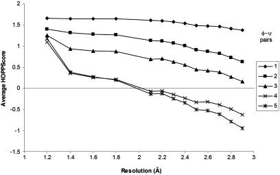
The most-recognized indicator of overall structural quality is the resolution of a crystal structure. To determine what range of resolution we might expect for a particular HOPPscore value we tested each of the resolution bins (1.2–3.0 Å) from the crystal structures in the PDBselect data against the reference hash table for structures >1.2-Å resolution (Fig. 3).

Fig. 3.

HOPPscore values correlate with resolution. Average HOPPscore values are collected for structures falling within a resolution bin. Scores for all fragment lengths (one to five φ–ψ pairs) inversely vary with resolution. The score dependency on resolution is greatest for longer lengths. The variable grid size is 12°, and the resolution set is 1.2 Å. (Note: the 1.2-Å bin is a self-score, i.e., scored with a hash table constructed from the identical 1.2-Å structures.)

Comparing model scores to their high-resolution CASP targets.

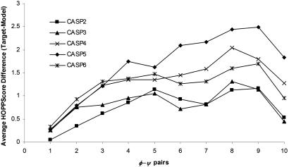
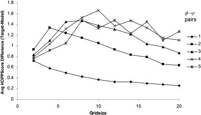
As a control, we collected only the high-resolution targets with resolutions >1.8 Å and compared their scores with each of the predicted models. We assumed the targets were of good structural quality and would score better than their models. The conformational hash table used for scoring was derived from structures >1.8 Å (a threshold comparable to the targets being tested). Fig. 4 shows the results of the score comparison for k values of 1–10 for CASP6 models with a default grid size of 12°. The grid size is an important parameter because it determines the coarseness with which structures are scored. If conformational space is binned too finely, relatively minor difference in conformation will be recognized as completely different structures. On the other hand, a grid size that is too coarse leads to overgeneralization of conformations. For each k = 1. . . 10, the variable, grid size, is tested between 2° and 20°. The range of grid size and k was then tested on the CASP4 models. The maximal difference in score (Fig. 5) provides us with a default grid size of 12° value.

Fig. 4.

Comparing the scores of CASP models to their high-resolution targets. For each fragment size from 1 to 10 φ–ψ pairs both the predicted model and the corresponding experimental target (for high-resolution structures ≤ 1.8 Å) HOPPscore values are calculated and the difference between scores is tallied. Average scores for each of the CASP trials are displayed. Variable grid size = 12°, and resolution set = 1.8 Å.

Fig. 5.

Best grid size for binning conformational space. For grid size values 2–20° and a fragment size of 1–10 φ–ψ pairs the CASP4 predicted model and the corresponding experimental target (high-resolution structure) HOPPscore difference scores are calculated. Decent choices for grid size lie in a range of 8° to 12°. Resolution set = 1.8 Å.

HOPPscore correlates with resolution.

The HOPPscore values we obtained for each resolution bin highly depended on the resolution (Fig. 3). The worse the resolution (i.e., higher values) the worse the HOPPscore values obtained. The longer fragments lengths exhibited the greatest dependency on resolution. The slope decreased much more quickly at higher Å (lower-resolution) levels for four and five φ–ψ pairs, indicating the greater degree of sensitivity to resolution. This result is particularly useful, because it indicates that quality analysis of experimental structures might provide more information if longer fragment lengths are used, as opposed to the single φ–ψ pair analysis commonly used now in procheck.

Scoring models of high-resolution targets.

We show that the predicted models of high-resolution CASP targets score significantly lower than the targets themselves. Fig. 4 shows the results of the scoring by individual CASP trial separately. The horizontal score axis is a difference score (experimental target score minus model score). If a model scores better than its experimental target, then the resulting difference score is <0. A global peak in scoring is reached at a fragment size of eight or nine φ–ψ pairs. However, these score differences are also obtained in several of the CASP trials using a shorter fragment length of four or five φ–ψ pairs. This fragment length provides a reasonable discrimination between poorly fitting models from all of the CASP trials and experimental targets. A fragment length of one φ–ψ pair results in the least amount of discrimination for all five CASP trials. This finding is most likely caused by the inclusion of φ–ψ restraints in the CASP predictors’ optimization algorithms.

A reasonable grid size was found by scoring the CASP6 models against their high-resolution targets and using a set of grid values from 2° to 20° (Fig. 5). The best grid size appears to be a range of values between 8° and 12°. These values are actually fairly large, because the bin size also depends on the fragment length. For instance, the angles within a fragment four φ–ψ pairs long would be placed into bins of 48° wide when grid size is 12°. See Materials and Methods.

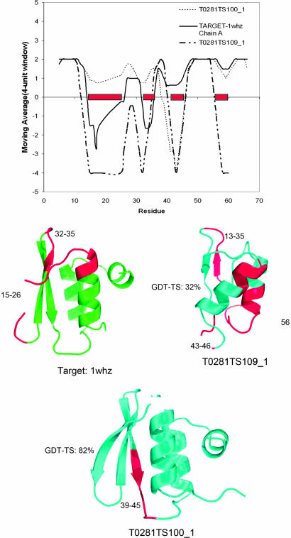
Some scoring examples are shown in Table 2to reveal the utility of HOPPscore for measuring model quality. We scored both model and target structure by using k = 4, grid size = 12°, and resolution set = 1.8 Å and compared the score differences to the global distance test total score (GDT-TS), which is a CASP measure of model quality. GDT-TS is defined as the percent of model residues matching the target structure residues within 2 Å. HOPPscore and GDT-TS values are not perfectly correlated (R² ≈ 0.05), because our scoring method contains no target structure information. However several of the models with GDT-TS <35% also have comparatively large HOPPscore differences. In general, HOPPscore values for model structures <0.50 (k = 4) should be re-examined very carefully. Two specific models are profiled in Fig. 6, showing which regions of the target and models are poor-scoring. In the target 1whz chain A, there are several poor-scoring regions, turns at residues 17–19 and 35–36. In model T0281TS100_1, the poorest-scoring region ranges from 42 to 49 in a coil between a sheet and helix. Despite this segment, this model has a fairly good GDT-TS (>80%) and a good HOPPscore. The majority of the residues in T0281TS109_1 score poorly. Fig. 6 also shows structural representations highlighting poorly scoring regions.

Table 2.

HOPPscore examples, scoring with k = 4 (φ−ψ) pairs

CASP model	Target Protein Data Bank	Residues	GDT-TS	HOPPscore model (φ−ψ)4	HOPPscore target (φ−ψ)4	Difference (φ−ψ)4	scop class
T0281TS109_1	1 whz: A	5–18, 25–60	31%	−0.79	0.89	1.00	α+β or α/β
T0281TS100_1		5–18, 25–66	82%	0.81	1.08	0.27
T0130TS001_1	1no5:A	7–101	55%	.35	1.35	1.00	α+β or α/β
T0130TS132_1		7–101	25%	0.64	0.98	0.34
T0137TS001_1	1o8v:A	70–129,2–29,35–58	86%	.09	1.02	.93	All β
T0137TS548_1		65–129, 2–58	14%	−3.04	0.99	4.03
T0073TS009_1	1g6u:A	2–44	82%	0.79	1.77	0.98	All α
T0073T155_1u		2–43	62%	0.23	1.85	1.57
T0083TS005_1	1dw9:A	3–62	30%	1.69	1.32	−0.37	All α
T0083TS009_1		3–72	10%	0.61	1.39	0.78

GDT-TS, a CASP measure of model quality; percentage of model Cα carbons within 2 Å of distances from target structure.

Fig. 6.

Moving average-score profiles and low-scoring regions in model and target. Both target and model fragments are scored with variables k = 4, grid size = 12°, and resolution set = 1.8 Å (“See Fragment” scores range from −4 to 2). Overall scores for Protein Data Bank files are summarized in Table 2. High-scoring model T0281TS100_1 (dashed line) is compared with its target 1whz (solid line). Low-quality portions of the models are observed in residues 45–50 and near residues 17 and 34 in the target structure. Scoring of model T0281TS109_1 (dot-dash line) shows that much of the structure is of low quality. Low-scoring regions (<0) in models T0281TS100_1, T0281TS109_1, and target 1whz are highlighted in red.

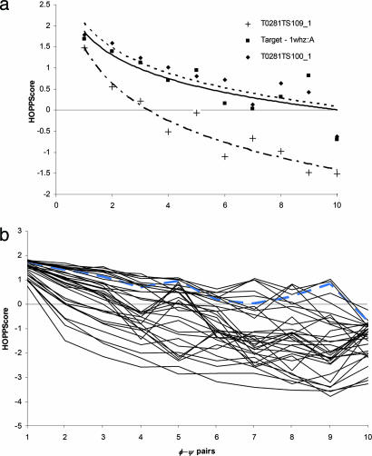
In addition, the scoring for k = 1–10 for the above 1whz models is plotted as a logarithmic curve in Fig. 7a, fitting the form m · ln(x) + b. The slope, m, of these curves provides a single value to access query structures quality for all fragment lengths. The curves of T0238TS100_1 and 1whz are nearly identical with similar slope (m = −0.80). The “poor” model has a descending slope steeper than 1whz (m = −1.26). Typical values for suspect models show slopes < −1.00. When scores for the range of k values (from 1 to 10) for several models (Fig. 7) are compared against the target, we can see that the target scores much better than the majority of the models. However, a few models score slightly better than the target probably because they are built with a larger percentage of commonly observed fragments.

Fig. 7.

Scoring with longer fragment lengths. (a) With grid size of 12° and resolution set of 1.8 Å, models T0281TS100_1 (dashed line), T028TS109_1 (dot-dash line), and target 1whz (solid line) were scored for k = 1–10. Best-fit logarithmic curves [m · ln(x) + b] for T0281TS100_1 (m = −0.86) and the target nearly match (m = −0.81). From k = 1 the curve for T028TS109_1 (m = −1.26) descends faster. (b) Forty models from several CASP groups are scored and compared with the target, 1whz (blue line). Most of the models scored poorly for k ≥ 2. Several models scored as well as or better than the target because they were constructed with commonly observed structural fragments.

Conclusion

We have developed a tool for protein structure analysis, which can be used to assess the quality of structural models and identify regions of predicted structures that contain “unnatural” building blocks or rarely observed structure. The fact that model structures consistently score worse with HOPPscore than target experimental structures is convincing evidence that many models are constructed with unnatural structural fragments. However, we want to stress that our quality scoring method is an independent “analysis” tool for models in the absence of experimental target structures or for experimental structures determined at low resolution. As long as HOPPscore is not incorporated into any refinement procedure for structure prediction, it can be used to check the quality of the prediction and supplement other methods as a form of “independent audit.”

Materials and Methods

A hash table is the most efficient way to “bin” conformations in multidimensional space, because we can ignore empty bins. Conformations are placed in the hash, hash table, by using a simple scheme:

For each conformation (or fragment) found in all of the structures at a given threshold resolution level, we have a vector V. A unique key is generated, via the function createKey(), representing that conformation, and each time that conformation is found the value stored in the hash table is incremented, yielding a conformational frequency. The ideal computer language for implementing such a hash table is perl because of its built-in hash data type. The function createKey() converts each vector, V, into a character string:

The angle value of each element i of V is rounded down to one of the 360/(k*gridSize) intervals. The parameter, grid size, determines the coarseness of the “binning” in the hash table. The unique key is then created by concatenating all of the rounded angle values together with a text separator, “_”. For example the vector V = 〈30,60,150,90〉 with grid size = 12° and k = 2 would have a unique key of _24_48_144_72. The size of the bin is a function of both k and grid size. The longer the fragment length, k, the coarser the bin.

Abbreviations

HOPP

higher-order φ–ψ

CASP

Critical Assessment of Protein Structure Prediction

GDT-TS

global distance test total score.

References

- 1.Lakowski R. A., MacArthur M. W., Moss D. S., Thornton J. M. J. Appl. Crystallogr. 1993;26:283–291. [Google Scholar]
- 2.Morris A. L., MacArthur M. W., Hutchinson E. G., Thornton J. M. Proteins. 1992;12:345–364. doi: 10.1002/prot.340120407. [DOI] [PubMed] [Google Scholar]
- 3.Shortle D. Protein Sci. 2002;11:18–26. doi: 10.1110/ps.ps.31002. [DOI] [PMC free article] [PubMed] [Google Scholar]
- 4.Shortle D. Protein Sci. 2003;12:1298–1302. doi: 10.1110/ps.0306903. [DOI] [PMC free article] [PubMed] [Google Scholar]
- 5.Sims G. E., Kim S-.H. Proc. Natl. Acad. Sci. USA. 2005;102:618–621. doi: 10.1073/pnas.0408746102. [DOI] [PMC free article] [PubMed] [Google Scholar]
- 6.Dill K. A. Biochemistry. 1985;24:1501–1509. doi: 10.1021/bi00327a032. [DOI] [PubMed] [Google Scholar]
- 7.Tendulkar A. V., Sohoni M. A., Ogunnaike B., Wangikar P. P. Bioinformatics. 2005;21:3622–3628. doi: 10.1093/bioinformatics/bti621. [DOI] [PubMed] [Google Scholar]
- 8.Levinthal C. J. Chim. Phys.-Chim. Biol. 1968;65:44–45. [Google Scholar]
- 9.Ramachandran G. N., Sasisekharan V. J. Mol. Biol. 1963;7:95–99. doi: 10.1016/s0022-2836(63)80023-6. [DOI] [PubMed] [Google Scholar]
- 10.Pappu R. V., Srinivasan R., Rose G. D. Proc. Natl. Acad. Sci. USA. 2005;97:12565–12570. doi: 10.1073/pnas.97.23.12565. [DOI] [PMC free article] [PubMed] [Google Scholar]
- 11.Moult J., Fidelis K., Zemla A., Hubbard T. Proteins Struct. Funct. Genet. 2003;53:334–339. doi: 10.1002/prot.10556. [DOI] [PubMed] [Google Scholar]
- 12.Hobohm U., Sander C. Proteins. 1994;27:244–247. [Google Scholar]
- 13.Kabsch W., Sander C. Biopolymers. 1983;22:2577–2637. doi: 10.1002/bip.360221211. [DOI] [PubMed] [Google Scholar]
- 14.Smith T. F., Waterman M. S. J. Mol. Biol. 1981;147:195–197. doi: 10.1016/0022-2836(81)90087-5. [DOI] [PubMed] [Google Scholar]