Three-Dimensional Fluid-Structure Interaction Simulation of Bileaflet Mechanical Heart Valve Flow Dynamics

Abstract

The wall shear stress induced by the leaflet motion during the valve-closing phase has been implicated with thrombus initiation with prosthetic valves. Detailed flow dynamic analysis in the vicinity of the leaflets and the housing during the valve-closure phase is of interest in understanding this relationship. A three-dimensional unsteady flow analysis past bileaflet valve prosthesis in the mitral position is presented incorporating a fluid-structure interaction algorithm for leaflet motion during the valve-closing phase. Arbitrary Lagrangian–Eulerian method is employed for incorporating the leaflet motion. The forces exerted by the fluid on the leaflets are computed and applied to the leaflet equation of motion to predict the leaflet position. Relatively large velocities are computed in the valve clearance region between the valve housing and the leaflet edge with the resulting relatively large wall shear stresses at the leaflet edge during the impact-rebound duration. Negative pressure transients are computed on the surface of the leaflets on the atrial side of the valve, with larger magnitudes at the leaflet edge during the closing and rebound as well. Vortical flow development is observed on the inflow (atrial) side during the valve impact-rebound phase in a location central to the leaflet and away from the clearance region where cavitation bubbles have been visualized in previously reported experimental studies.

INTRODUCTION

Mechanical valve implants to replace the diseased heart valves is a common treatment employed today, but patients with these implants need to be under long-term anticoagulant therapy in order to minimize problems related to thromboembolic complications. In the last decade, numerous studies have implicated the flow induced stresses during the valve-closing phase with damage to platelets and thrombus initiation.^18,21 Cavitation bubble development because of the presence of large negative pressure transients^{5,16,17,22,28} on the inflow side of the leaflet edge and subsequent collapse of the bubbles may also contribute to platelet activation.

Numerous experimental studies and numerical simulations have been reported in the literature to analyze the flow dynamics during valve-closing phase, providing valuable insight on the flow dynamics near the valve leaflets. Experimental studies have demonstrated the presence of large negative pressure transients at the leaflet edge at the instant of valve closure and initiation of cavitation bubbles in this region.^{6,8,15–17,28} Subsequently, in vivo studies have confirmed the presence of such large negative pressure transients in the atrial side during mechanical valve closure in the mitral position in an animal model.^6,14 Significant damage to formed elements in blood during valve-closing phase have been reported²¹ and the presence of short-lived 3D vortex in the vicinity of the leaflets during the closing phase and subsequent leaflet rebound¹⁸ have also been demonstrated through in vitro experimental studies.

Computational fluid dynamic (CFD) analysis during the last few degrees of leaflet closure^3,24 of mechanical heart valves demonstrated the presence of negative pressure transients on the inflow side and its subsequent enhancement during the valve rebound phase. Previous studies from our laboratory^1,20 have presented the simulation of the bileaflet valve dynamics during the valve-closing phase and the results demonstrated the large negative pressure transients in the atrial side as well relatively large wall shear stresses in the clearance region at the instant of valve closure. However, in these simulations, the fluid-structure interaction computations were avoided by the specification of the leaflet motion from experimental data.

Fluid-structure interaction analysis for tissue valve dynamics have been reported^2,11–13 employing the fictitious domain method associated with the finite element discretization employing a fixed mesh while the motion of the leaflet was incorporated. The model has been applied to the open and closed phases of tissue valve function, and yet to be applied to the transitional phase of tissue valve function involving the complex leaflet motion. Cheng et al.⁹ presented a fluid-structure interaction model to predict the leaflet motion induced by the forces exerted on the leaflet because of the flow dynamics. This two-dimensional (2D) model of a bileaflet valve was employed to simulate the closure and the rebound phases of the leaflet during valve closure and results demonstrated the enhanced negative pressure transients and wall shear stresses near the leaflet edge during the rebound phase. In the present work, the simulation by Cheng et al.⁹ are extended to the three-dimensional (3D) geometry of the bileaflet valve geometry. The results are compared and contrasted with the results from the 2D fluid-structure interaction simulation and the importance of 3D simulations in the analysis of detailed fluid dynamics is discussed.

NUMERICAL METHOD

Solution of the blood flow through a bileaflet heart valve is based on U2RANS CFD code employing a laminar flow formulation of an incompressible Newtonian fluid with properties representative of whole human blood (density of 1056 kg/m³ and a viscosity coefficient of 0.0035 kg/ms). This code has been validated for analysis with moving boundaries and employed for analysis of several engineering problems¹⁹ and also employed in the mechanical valve simulations²⁰ in our laboratory. In the bileaflet valve geometry, the two leaflets are symmetric with respect to the valve centerline parallel to the pivot axis. Each leaflet is also symmetric along the diameter vertical to the pivot axis. Taking advantage of the symmetry, the 3D model consisted of half of one leaflet as shown in Fig. 1. The leaflet in the fully closed position lies on the x–z plane with the y-coordinate indicating distance from the leaflet surface on the atrial (inflow) side of the valve. The nominal dimensions of the leaflet geometry for this simulation represented a 25-mm Medtronic ADVANTAGE^®bileaflet valve [Fig. 1(c)] where the leaflet rotates 63.8° from the fully opened position. In this simulation, the leaflet fully open position was specified as 0° [0.2° with respect to y-axis in Fig. 1(b)] and the fully closed position as 63.8° (64° with respect to y-axis) as shown in the 2D view from the top shown in Fig. 1(b). The atrial chamber length L1 of 18 mm and the ventricular chamber length L2 of 20 mm were specified in the simulation. The flow chamber was represented by one quarter of a circular pipe with a diameter of 24.52 mm. The solid arrow in Fig. 1(b) indicates the flow direction during the leaflet closing phase and the dotted arrow indicates the leaflet rebound direction. In the 2D simulation reported previously, the geometry corresponded to the view shown in Fig. 1(b) where the leaflet was treated as a rectangular plate with a unit width with the flow chamber being represented by two parallel plates.

FIGURE 1.

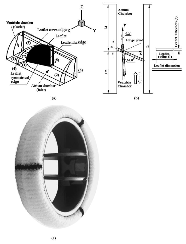
Three-dimensional (3D) simulation model of the mechanical heart valve for the fluid-structure interaction simulation. The leaflet in the fully closed position lies on the x –z plane with the y -coordinate indicating distance from the leaflet surface on the atrial (inflow) side of the valve. (a) The 3D geometry of the one half of one leaflet in the flow chamber with the ventricular and atrial sides indicated. The numbers represent the various blocks in the mesh reconstruction for the flow dynamic simulation; (b) The top view of the simulation geometry showing the fully open and closed positions of the leaflet as well as the leaflet dimensions; (c) Photograph of the Medtronic ADVANTAGE® bileaflet valve from which the nominal dimensions for the simulation were obtained.

The solution procedure for the fluid-structure interaction problem is described in Cheng et al.⁹ and is briefly described here in the interest of continuity. The governing equations for the fluid motion consisted of the 3D equations of continuity and momentum. In addition the space conservation law as described in Lai¹⁹ is employed for the moving boundary analysis. The leaflet rotation can be described by the relationship,

$$\frac{d^2\theta }{d{t}^2}=\frac{M}{I_{\text{o}}}$$ (1)

In the equation, θ(t) is the opening angle, indicating the leaflet position at any instant t; I_o is the moment of inertia of the leaflet about the pivot; M is the total momentum acted on the leaflet from the external forces inducing the leaflet motion. The external momentum can be calculated as

$$M=M_{\text{G}}+M_{\text{p}}+M_{\text{f}}$$ (2)

M_G is the momentum resulting from the buoyancy and the gravitational force and is given by

$$M_{\text{G}}=g*V*({\rho }_l-{\rho }_f)*\mathrm{\hspace{0.17em} }\text{cos}(\theta )*(l/2-a)$$ (3)

Here g is the acceleration due to gravity, V is the leaflet volume; ρ_l is the density of leaflet (2000 kg/m³); ρ_f is the density of the fluid (1056 kg/m³); and “l” and “a” are the leaflet radius (13.16 mm) and pivot length (1.79 mm), respectively as shown in Fig. 1(b). The leaflet thickness “e” was specified as 0.899 mm and the moment of inertia as 3.3e–9 kg m². M_p is the momentum resulting from the blood pressure, and M_f is the momentum resulting from the friction between the leaflet and the flowing blood. The values of M_p and M_f at any given instant of leaflet rotation are obtained from the computed flow field.

To obtain the flow field, the valve-closing process can be divided into incremental time steps. In each step, the blood pressure and the friction force computed from the previous time step is integrated over the leaflet surface to compute the momentum due to the pressure and shear stress. The leaflet governing equation of motion [Eq. (1)] is solved using the fourth-order Runge–Kutta method to determine the new position of the leaflet. Once the leaflet position is calculated, a new mesh is constructed and the grid velocity computed, and the fluid governing equations are solved again to determine the flow field for the new geometry.

Leaflet Rebound

The leaflet will impact against the valve seating lip at the instant of valve closure. After impact, the leaflet will bounce back from the housing. The governing equation of leaflet dynamics during impact can be expressed as

$${\omega }_2=-r{\omega }_1$$

where r is the coefficient of resilience that depends upon the material of the leaflet and the valve housing. ω₁ and ω₂ are the angular velocities before and after impact, respectively. The coefficient of resilience is specified as 0.5. Experimental data on the measurement of coefficient of resilience was not available and hence we adopted a typical value reported in the literature for leaflet impact simulation.¹⁰

Mesh Regeneration and Grid Independence

The flow field was divided into eight blocks [as indicated by the numbers in Fig. 1(a)] for the computational analysis. The meshes in the blocks were generated by using the GRIDGEN preprocessor with grids being clustered near the leaflet in order to ensure solution accuracy in the deterministic flow field. Typical mesh representation for the various blocks for a given leaflet position are shown in Fig. 2. Effective mesh regeneration process is necessary to solve the moving boundary resulting from the rotation of the leaflets, and grid velocity must be computed accurately for the flow field computation. The meshes at the leaflet full open (0.2°), and the full closed (64°) positions, as well as at a number of selected intermediate leaflet locations (5°; 11°; 18°; 26°; 34°; 41°; 47°; 52°56°; 59°; 61°; 62.5°; and 63.5°) were pregenerated and saved. It can be noted that the pregenerated meshes were also clustered near the leaflet impact due to the increase in the angular velocity of the leaflets during the latter stages of valve closure. In the computation process, new mesh reconstructions at each time step will be based on these saved meshes. The total number of grid points employed in the solution was 226090 with 210000 cells compared to 9830 grid points with 9550 cells employed in our previous 2D simulation.⁹ These numbers were based on our simulations with similar geometries that have been previously employed for valve closure simulation in our laboratories.^1,20 We ran the simulation by doubling the mesh size and the results on the magnitudes of the computed velocity and wall shear stresses were within 1% of the results obtained with the mesh density given above.

FIGURE 2.

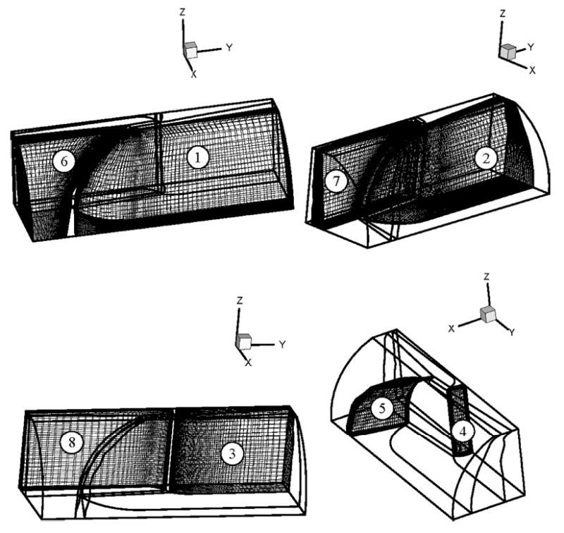
Typical block mesh plots employed in the simulation.

Solution Procedure

The solution starts with the quiescent initial conditions with the valve in the fully open position. The ventricular pressure rise rate during the closing phase^8,23 $\frac{dp}{dt} {|}_{\text{cl}}$ was specified as 2000 mmHg/s and the atrial pressure was assumed to be constant at zero as shown in Fig. 3. A temporal convergence criterion study was performed in the 2D simulations by running the simulations at 6.0, 3.0, and 1.5 × 10⁻⁵ s and comparing the computed results of the valve-closing position as a function of time. The results for the smallest two time steps were identical and hence we employed a time step of 3.0e–5 s for both the 2D and 3D simulations to yield results of sufficient accuracy with reasonable time and memory requirements.

FIGURE 3.

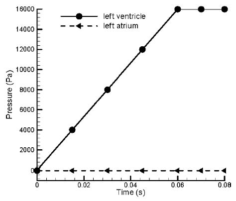
The left ventricular and the atrial pressures used in the flow simulation during the closing phase of the mechanical valve in the mitral position.

The solution procedure in the simulation is given below:

1. With the initial mesh known and the quiescent initial conditions given, the fluid equations are solved for the first time step with the application of the ventricular pressure rise.

2. The dynamic equation of the leaflet motion [Eq. (1)] is then solved to obtain the new leaflet position (angle) based on the results of the flow field.

3. The mesh corresponding to this new leaflet position is then obtained through interpolation, using the two neighboring meshes that have been generated earlier.

4. The surface nodes on the new leaflet position is recomputed as the product of the leaflet rotation angle computed in Step 2 and the radial distance of the node from the pivot point. The interpolated mesh is modified slightly to match with the leaflet surface nodes.

5. An elliptic solver is further applied to the entire mesh. The elliptic solver is to solve the Laplacian equation, ▿²δ = 0, where δ is the displacement of each grid point. A “final” mesh is obtained after the solution of the Laplacian equation using the successive over-relaxation (SOR) method.

6. At the instant of leaflet impact with the seating lip, leaflet equation of motion is substituted by the leaflet rebound equation to calculate the leaflet rebound velocity and new leaflet position.

The above-mentioned Steps 1–6 are repeated to obtain all solutions in a time-accurate fashion.

RESULTS

Closing Process

The simulation begins from the fully opened position, and the computed leaflet opening angle vs. time are plotted in Fig. 4 along with the 2D numerical simulation results⁹ under the same simulation conditions. Experimental data, obtained in a pulse duplicator with a glycerin–water solution with similar fluid parameters, during the closing phase employed in²⁰ are also superposed in this figure for comparison. In the experimental data, it is difficult to find the exact time when the leaflet begins to open. Hence, the time interval prior to measured leaflet motion toward closure in the experimental data was superposed with the leaflet fully open position from the simulations. The leaflet is closing more rapidly with the 3D simulation compared to that of the 2D simulation. The rate of closure from the simulation curves between the 30° to the fully closed position of the valve in the 2D simulation was computed to be 8825° per second compared to 9940° per second for the 3D simulation. The maximum rate of closure from the experimental data in the same interval was 10890° per second and that value is closer to the magnitude for the 3D simulation. In the 2D simulation, the leaflet dimension was rectangular corresponding to the leaflet radius at the symmetrical plane. Because of the differences in the geometry of the leaflets between the 2D and the 3D models and thus the fluid dynamics during closing, our simulation shows that the leaflet closure is earlier with the 3D model compared to the 2D model. The computed leaflet position after the leaflet impact and rebound are also included in the figure. The experimental data were not available during the leaflet impact-rebound event. The 2D simulation with the rectangular geometry for the leaflet predicts a larger rebound compared to that in the 3D simulation with the more accurate representation of the leaflet geometry with the rebound model employed in this study.

FIGURE 4.

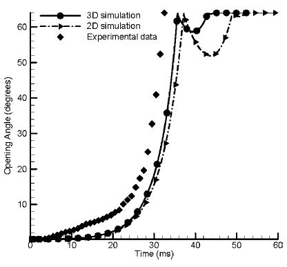
The computed leaflet position as a function of time for the 3D simulation compared with the in vitro experimental data and 2D simulation results under the same conditions. Data on valve rebound was not available in the experimental study.

Pressure Field during the Closing and Rebound Phase

The unsteady 3D simulation results can be used to compute the detailed pressure and velocity field in the vicinity of the leaflet during the closing phase that occurs in about 30 ms as shown in Fig. 4. Since the most significant local negative and positive pressures occur around the leaflet surfaces, the pressure contours on the leaflet surfaces are displayed in Fig. 5. The local negative pressures are initially generated above the leaflet edge in the closing process [Fig. 5(a)], then the negative pressures increase and the largest negative pressure point is found at the leaflet edge in the symmetry plane (Fig. 5b). The local negative pressure region extends to the whole leaflet inflow (atrial) surface and lasts until the instance of leaflet impact [Fig. 5(c)] and the subsequent rebound [Fig. 5(d)]. The negative pressures on the leaflet surface on the atrial side were below −75 mmHg at about 2 ms before impact and the pressures become more negative with the leaflet closer to the impact position. Large local positive pressure region is observed on the outflow (ventricular) side of the leaflet. At the leaflet position of 63.73°, just before the leaflet moves to the fully closed position, the maximum negative pressure computed is −597 mmHg with the corresponding maximum positive pressure of 612 mmHg. The maximum local negative pressure magnitudes computed during the closing phase before the impact is above the vapor pressure for blood (−720 mmHg at 37°C) and hence is not likely to induce cavitation bubbles. The largest negative pressure during the first rebound is computed to be −5291 mmHg and the corresponding positive pressure at the ventricular side computed as 4201 mmHg. Negative pressures beyond −760 mmHg computed in this simulation are not physically meaningful and are because of the single-phase flow analysis employed in the model. To analyze the formation of cavitation bubbles as the negative pressure goes below the vapor pressure for the fluid, a two-phase model will be required and was not employed in this simulation. However, it should be pointed out that our results agree with the previous studies that suggested that cavitation bubble formation is more likely after the leaflet impact and subsequent rebound.^3,24 In the second impact-rebound phase computed in the simulation, the significant local negative pressure still exists, but the magnitudes and the duration are much smaller and hence not included in the figure. The large negative pressures computed in the simulation, ranging from −750 mmHg in most of the leaflet surface on the atrial side with maximum negative pressures at the leaflet edge, are present for less than 2 ms and agree with the experimental studies in which the cavitation bubbles formed with mechanical valves during the valve closure are observed to collapse within the same time period.

FIGURE 5.

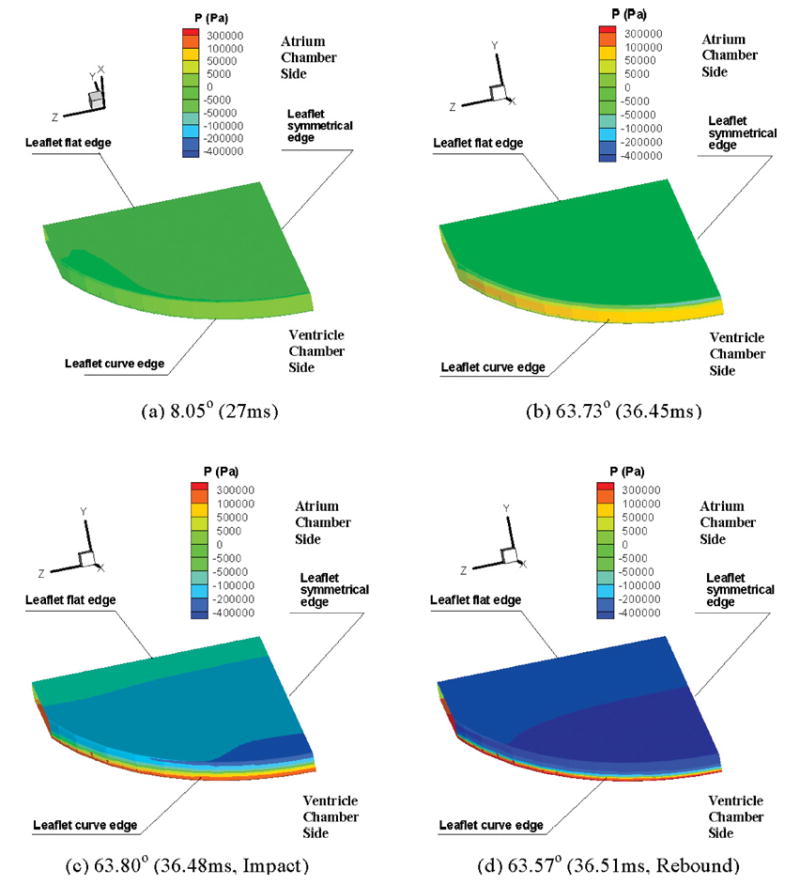
Pressure contours during the leaflet closing process: (a) Pressure contour at 8.05° leaflet position in the closing process (P_min = −12 mmHg, P_max = 54 mmHg); (b) Pressure contour at 63.73° in the closing process (P_min = −597 mmHg, P_max = 612 mmHg); (c) Pressure contour at 63.80° at the impact instant (P_min = −2273 mmHg, P_max = 1513 mmHg); (d) Pressure contour at 63.57° in the first rebound process (P_min = −5291 mmHg, P_max = 4201 mmHg). The color plots use the same scale for the four time points and the scale legend are given in the units of Pascal.

A comparison of the computed pressure distribution between the 2D and the 3D models revealed a qualitatively similar pattern even though the magnitudes of the maximum negative and positive pressures differed between the two simulations. In Fig. 6, the maximum local negative and positive pressure magnitudes in the valve symmetry plane during the leaflet closing-impact-rebound process for the 2D and 3D simulations are compared. The magnitudes of the maximum negative and positive pressures are larger in the 2D simulation compared to that for the 3D simulation and once again can be attributed to the difference in the leaflet geometry between the 2D and 3D simulations. In Fig. 4, it was observed that the rebound distance for the 2D simulation is larger compared to that for the 3D simulation. The positive and negative pressure spikes in the 2D simulations occurring at a later time compared to that for 3D simulation in Fig. 6 are also consistent with the larger distance traveled by the leaflet during the rebound process observed in the 2D simulation.

FIGURE 6.

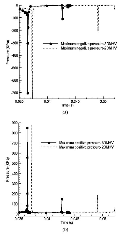
Comparison of the maximum positive and negative pressures in the leaflet closing process: (a) Maximum negative pressure vs. time; (b) Maximum positive pressure vs. time.

Velocity Profiles and Wall Shear Stress in the Clearance Region

The pressure contours demonstrated that the maximum local negative and positive pressure regions are both located around the leaflet edge in the vicinity of the clearance between the leaflet and valve housing. These large pressure gradients induce large local blood velocity and wall shear stress in this region. Figure 7(a) and (b) show the velocity profiles across the clearance region as the fluid moves into the atrial chamber during the closing phase and after the first rebound. In these figures, the clearance region is viewed from the atrial side with the valve symmetry plane to the right of the figure. The numbers in the figure correspond to the velocity magnitudes indicated in the figure legend in the clearance region in the plane at the middle of the leaflet thickness. Figure 7(a) indicates the velocity distribution in the clearance region during the valve-closing phase and Fig. 7(b) the corresponding plot after the first rebound of the leaflet. It can be observed that the maximum velocities through the clearance region are larger after the first rebound compared to those in the initial closing phase. The wall shear stress distribution on the leaflet edge in the clearance region at the corresponding leaflet positions is shown in Fig. 8(a) and (b). In these figures, numbers on the leaflet edge corresponds to the magnitudes of the wall shear stresses shown in the legend. As can be observed, larger wall shear stresses are observed closer to the symmetry plane of the leaflet and the magnitudes of wall shear stress exceed 4 kPa in the clearance region during the closing and rebound phases. The maximum fluid velocity in the clearance region during this phase of leaflet motion is around 28 m/s and the maximum wall shear stress exceeds 16 kPa. The platelet activation potential has been related to the magnitude of the WSS and the duration for which the platelets are exposed to them.^4,26 The maximum WSS–time plot in the clearance region during the first rebound is shown in Fig. 9. Using a value of 10 kPa for the WSS and 0.002 s for the duration of the stress from this plot, WSS–time product of 20 Pa·s is obtained as representative of the area under the curve. This value exceeds the magnitudes of 3.5 Pa·s²⁶ suggested for procoagulant platelet factor 3 release indicative of platelet activation. These simulations do support the claim that WSS–time magnitudes present during the valve-closing phase in the clearance region may be one of the dominant factors inducing thrombus formation.

FIGURE 7.

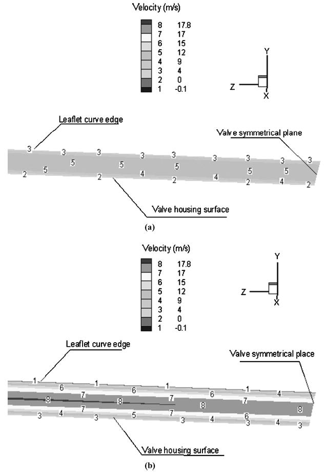
Fluid velocity distribution within the clearance region between the leaflet edge and the valve housing. The clearance is being viewed from the atrial side with the valve symmetry plane to the right side of the figure. Note that these figures are enlarged for clarity; therefore the leaflet curve edge appears as a straight line. (a) With the leaflet position at 63.73° in the closing phase (V_max = 17.45 m/s); (b) with the leaflet position at 63.57° in the first rebound phase (V_max = 27.67m/s).

FIGURE 8.

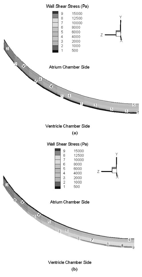
Wall shear stress distributions on the leaflet arc face of two different leaflet’s positions: (a) with the leaflet position at 63.73° in the closing phase (Max WSS = 11168 Pa); (b) with the leaflet position at 63.57° in the first rebound phase (Max WSS = 17488 Pa).

FIGURE 9.

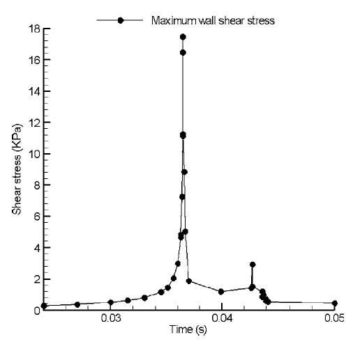
Maximum wall shear stress (WSS) vs. time plot in the clearance region during the first rebound of the leaflet after impact.

Vortex Formation in the Atrial Chamber during Valve Closure and Rebound

The 3D model was also used to compute the detailed flow field on the inflow side of the leaflet during the closing and rebound phase and such detailed analysis cannot be studied in a 2D model. Figure 10 illustrates the vortex formation on the atrial side of the leaflet during the closing motion of the leaflet and subsequent rebound. Figure 10(a) depicts the flow field prior to the impact of the leaflet (leaflet angle of 63.73°). As the jet-like flow emerging from the clearance region moves into the atrial chamber, the fluid comes into the negative pressure field near the leaflet shown in Fig. 4 and forms a large vortex near the center of the leaflet. The vortex expands and the center of the vortex moves closer to the leaflet at the instant of leaflet impact (63.8°) as shown in Fig. 10(b). During the rebound process [Fig. 10(c), −63.57°], the vortex has reduced in size and has moved closer to the leaflet surface. Because of symmetry, a similar vortex formation will also be present on the other half of the leaflet and such double vortex pattern has also been experimentally observed with the St. Jude valve.²⁵ Vortex formation near the major flow orifice of a tilting disc valve close to the periphery has been experimentally observed by Kini et al.¹⁸ With the bileaflet valves, the vortices appear away from the edge of the leaflet. In the bileaflet valves, experiments indicate cavitation bubbles to form generally near the peripheral clearance region^8,22 for ventricular pressure rise rates comparable to those used in this simulation and bubbles also being visualized near the central flow region between the leaflets at higher pressure rise rates.²⁷ Since the vortices appear away from either of these two regions in the simulation, the vortices may not play a significant role in the cavitation initiation with the bileaflet valve models.

FIGURE 10.

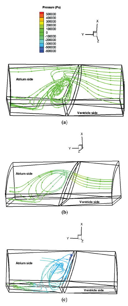
The stream line plots showing the vortex flow formation on the atrial side of the leaflet during the closing and rebound phases. The colors on the stream lines indicate the pressure distribution on the ventricular and atrial sides during the leaflet impact and rebound phases: (a) At the leaflet position of 63.73° closing phase; (b) At the leaflet position of 63.8° closing phase; and (c) At the leaflet position of 63.57° during the first rebound phase.

DISCUSSION AND CONCLUSIONS

A complete 3D fluid-structure interaction problem has been developed for the simulation of a mechanical valve closing dynamics in this study. The results on the predicted leaflet motion from the fully open position to the fully closed position compares reasonably well with the corresponding experimental data. The simulation results also show the presence of large negative pressure transients on the inflow (atrial) side of the valve leaflet and the corresponding positive pressure transients on the out-flow (ventricular) side of the leaflets. These data agree with in vitro experimental studies reported on the transient pressure measurements and cavitation bubble visualization with mechanical valves during the valve-closing phase. Our studies show that the negative pressures present on the inflow side during the leaflet closing motion are not below the vapor pressure for blood and hence may not initiate cavitation bubbles. However, the negative pressure magnitude is significantly increased at the instant of the leaflet impact and during the first rebound and hence may initiate cavitation bubble formation. These results also agree with the previous simulations suggesting the further enhancement of the negative pressure transients during the rebound phase.³ It should be pointed out that the negative pressure transients with magnitudes below the vapor pressure for blood computed in the simulation only indicates potential for the mechanical valve to cavitate during the leaflet closing/rebound phase. Other factors such as the presence of nucleus for cavitation bubble formation are necessary for incipience of cavitation.

The simulation results on the negative pressure transients exceed the absolute zero pressure and hence are not physically realistic. The reason for the same is the assumption of a single-phase fluid analysis. In the incompressible fluid dynamic analysis employed in this simulation, pressure is a dynamic quantity and a primitive variable not tied to fluid density and/or temperature. With this formulation, the pressure difference (rather than absolute pressure magnitudes) is physically meaningful and is dictated by the velocity field. This formulation is mathematically correct as long as the incompressibility assumption is valid. Physically, if the pressure magnitude falls below the vapor pressure for the fluid, cavitation and gas phase will be initiated leading to the breakdown of the incompressibility assumption. In the present simulation, large negative pressure transients only indicate that there is potential for cavitation to occur in that region. In order to study the details of the vapor pressure formation and cavitation bubble dynamics, a two-phase flow analysis is necessary and was beyond the scope of the present study. Nonetheless, the results indicate that the details of the dynamics of valve impact and rebound are necessary for a complete analysis of the mechanical valve closing dynamics.

With the large positive and negative pressure transients exerting a relatively large pressure gradient across the valve clearance region during the end of the valve-closing phase, relatively large flow velocity magnitudes are predicted in the clearance region. The computational simulation can provide details of the flow dynamics in this region where experimental measurements are impractical. These large fluid velocities also induce relatively large wall shear stresses on the leaflet edge. The product of the WSS and the duration of the stress in the clearance region determined from this simulation exceeded the magnitudes suggested to activate the platelets.^4,26 Previous experimental studies have suggested that damage to formed elements of blood in the clearance region during the reverse flow with the valve in the closed position is comparable to that in the forward flow phase.²¹ The present simulations suggest that during the transient closing and rebound of the leaflet, the wall shear stresses are significantly higher and hence may be an important factor in the thrombus initiation with implanted mechanical valves, a significant problem requiring long-term anticoagulant therapy for the patients.

Kini et al.¹⁸ presented an experimental study detailing the flow dynamics of a tilting disc valve during the valve closure and rebound. Their measurements performed using particle image velocimetry showed the formation of two confined vortices near the inflow surface in the major flow orifice region during the valve rebound phase. In the case of the closing mechanics for the tilting disc valves, negative pressures have been measured on the inflow side of the major orifice region while positive pressures are observed in the minor orifice region.⁷ Hence the negative pressures on the atrial side are more towards the major orifice region and hence the observed vortex formation is confined to the peripheral clearance region. On the other hand, the present simulation indicates, with the closure of the leaflet in the bileaflet valve model, negative pressure is observed through the entire inflow side surface of the leaflet and hence the vortex of a larger size occurs in the central region of the leaflet. Since the computed vortices are away from the peripheral clearance or the region between the two leaflets, this study suggests that the cavitation bubble formation in the bileaflet valves is not influenced by the vortices. However, in order to study the details of the vortical flow and its effect on the platelets and red blood cells, a simulation including a realistic 3D geometry of the atrium is necessary as discussed in the limitations section.

A comparison of the results from the 3D fluid-structure interaction simulation in the present work with the corresponding 2D simulation shows that the pressure and velocity field are comparable between the two simulations. However, the magnitude of the rebound predicted by the 2D simulation in this study is larger compared to that of the 3D simulation. Further more details of the flow dynamics in the atrial and ventricular chambers with the bileaflet mechanical valves may not be discerned from the 2D simulations. Our results suggest that the 2D simulation may be sufficient for the computation of the pressure and velocity field with mechanical valve design and development so that different leaflet configurations can be analyzed and an optimal design chosen before further prototype development and detailed experimental evaluation is undertaken. However for detailed local fluid dynamic analysis in the vicinity of the leaflet and the clearance region including the formation and behavior of the vortices near the leaflet surface, a 3D simulation is necessary.

Limitations of the Study

In order to simplify the problem, the bileaflet valve was assumed to be symmetrical and the analysis was performed with one half of one leaflet. We also neglected the geometry of the hinge mechanism about which the valve rotates. In reality the two leaflets will not have the exact dimensions and the geometry of the hinge may also vary from one side to another because of manufacturing tolerances. We consider this study to be the first step in the development of a fluid-structure interaction simulation of mechanical valve dynamics and further development of the simulation is important to include the details of the hinge geometry and assess the variability in valve and hinge geometry dimensions. With the inclusion of the hinge geometry, the leaflet-closing rate can be anticipated to alter due to the interaction between the leaflet ears and the hinge pocket. The nature and magnitude of alterations because of the presence of hinge geometry also needs to be assessed for a more accurate simulation.

In this simulation, we started the simulation with the leaflet in the fully open position and the fluid stationary as the initial condition. In reality, the valve moves from the closed position to the fully open position during diastole as the ventricular chamber is filled. Subsequently, with the ventricular pressure rise, the leaflet moves toward closure. We neglected this effect in this initial development of the simulation. However, the results from the simulation replicates the experimental studies in our laboratory where the cavitation dynamics of mechanical valves were assessed using a single closing event. It should be pointed out that the cavitation bubbles visualized with mechanical valves in our experiments with a single closing event are qualitatively similar to the bubble visualization with the same mechanical valves under pulsatile flow in Tarbell’s laboratory¹⁵ and hence we anticipate that our simulation describes the flow dynamics near the leaflets in the closing dynamics reasonably well. It will be necessary to include the motion of the leaflet through the entire cardiac cycle for a more realistic simulation.

Another limitation in the present simulation is in not incorporating the actual 3D geometry as well as the compliance characteristics of the left ventricular and the atrial chamber. The pressure transients measured in our in vitro studies were comparable with those measured with implanted mechanical valves in vivo⁶ and hence we anticipate that the flow dynamics near the leaflets during the closing phase are described reasonably accurately in our simulation. However, to characterize the vortical flow dynamics observed away from the leaflet in the atrial chamber and the effect of vortical flow on the platelets, incorporation of a realistic atrial geometry and compliance is necessary. The incorporation of a realistic ventricular geometry will also be essential to study the effect of the leaflet opening the effect of ventricular chamber flow on the subsequent leaflet closure.

We employed a weak coupling method in our fluid-structure interaction simulation and employed small time steps in the dynamic analysis to ensure accurate results. The explicit coupling method works well with the mechanical valve simulation with rigid leaflets as demonstrated by the agreement between the predicted and experimentally measured motion of the leaflets during the closing phase. The difference between weak and strong coupling is in their ability to promote numerical stability and both methods are numerically accurate. A simulation employing strong coupling will be necessary for the simulation to be extended to the bioprosthetic valves in order to accurately simulate the complex 3D motion of the leaflets during a cardiac cycle.

In this simulation, we concentrated on the valve-closing dynamics with particular attention to the fluid dynamics near the clearance region at the instant of valve closure. During the short time period of valve closure, very high velocity flow are observed in the clearance region between the valve housing and the leaflet edge with a gap width of 0.01 mm. Based on the fluid properties, gap width, and the largest velocity in the gap width, the Reynolds number is around 100 and hence we believe that we are reasonably accurate in employing a laminar flow simulation in this study. For a simulation of the valve function through the entire cardiac cycle, the flow can be anticipated to transition to turbulence for short durations in the overall cardiac cycle and a turbulence model will need to be incorporated. As pointed out earlier, the one phase fluid model was employed in this simulation and hence the analysis is incapable of describing the dynamics of the formation process vapor bubbles that have been visualized experimentally. Therefore, development of a two-phase fluid model will provide a more accurate simulation to analyze the phenomenon of cavitation initiation. In this initial attempt to develop a detailed 3D fluid–structure interaction problem, the geometric details of the hinge mechanism and the interaction of the leaflet and the valve housing in the hinge have been avoided. The incorporation of the details of the hinge geometry in the simulation is necessary before the effect of local geometrical differences on the fluid dynamics can be compared with the various models of the bileaflet mechanical valves and these developments are currently ongoing in our laboratory.

References

- 1.Aluri S, Chandran KB. Numerical simulation of mechanical mitral heart valve closure. Ann Biomed Eng. 2001;29:665–676. doi: 10.1114/1.1385810. [DOI] [PubMed] [Google Scholar]
- 2.Baaijens FPTA. fictitious domain/mortar element method for fluid-structure interaction. Int J Num Methods Fluids. 2001;35:743–761. [Google Scholar]
- 3.Bluestein D, Einav S, Hwang NH. A squeeze flow phenomenon at the closing of a bileaflet mechanical heart valve prosthesis. J Biomech. 1994;27:1369–1378. doi: 10.1016/0021-9290(94)90046-9. [DOI] [PubMed] [Google Scholar]
- 4.Bluestein D, Niu L, Schoephoerster RT, Dowanjee MK. Fluid mechanics of arterial stenosis: Relationship to the development of mural thrombus. Ann Biomed Eng. 1997;25:344–356. doi: 10.1007/BF02648048. [DOI] [PubMed] [Google Scholar]
- 5.Chandran KB, Aluri S. Mechanical valve closing dynamics: Relationship between velocity of closing, pressure transients, and cavitation initiation. Ann Biomed Eng. 1997;25:926–938. [PubMed] [Google Scholar]
- 6.Chandran KB, Dexter EU, Aluri S, Riehenbacher WE. Negative pressure transients with mechanical heart-valve closure: Correlation between in vitro and in vivo results. Ann Biomed Eng. 1998;26:546–556. doi: 10.1114/1.79. [DOI] [PubMed] [Google Scholar]
- 7.Chandran KB, Lee CS, Aluri S, Dellsperger KC, Schrack S, Wietins DW. Pressure distribution near the occluders and impact forces on the outlet struts of Bjork–Shiley convexo-concave valves during closing. J Heart Valve Dis. 1996;5:199–206. [PubMed] [Google Scholar]
- 8.Chandran KB, Lee CS, Chen LD. Pressure field in the vicinity of mechanical valve occluders at the instant of valve closure: Correlation with cavitation initiation. J Heart Valve Dis. 3(Suppl 1):S65–S75. discussion S75–S66, 1994. [PubMed] [Google Scholar]
- 9.Cheng R, Lai YG, Chandran KB. Two-dimensional fluid-structure interaction simulation of bi-leaflet mechanical heart valve flow dynamics. Heart Valve Dis. 2003;12:772–780. [PubMed] [Google Scholar]
- 10.Cheon GJ, Chandran KB. Dynamic behavior analysis of mechanical monoleaflet heart valve prostheses in the opening phase. J Biomech Eng. 1993;115:389–395. doi: 10.1115/1.2895502. [DOI] [PubMed] [Google Scholar]
- 11.De Hart J, Baaijens FP, Peters GW, Schreurs PJ. A computational fluid-structure interaction analysis of a fiber-reinforced stentless aortic valve. J Biomech. 2003;36:699–712. doi: 10.1016/s0021-9290(02)00448-7. [DOI] [PubMed] [Google Scholar]
- 12.De Hart J, Peters GW, Schreurs PJ, Baaijens FP. A two-dimensional fluid-structure interaction model of the aortic valve [correction of value] J Biomech. 2000;33:1079–1088. doi: 10.1016/s0021-9290(00)00068-3. [DOI] [PubMed] [Google Scholar]
- 13.De Hart J, Peters GW, Schreurs PJ, Baaijens FP. A three-dimensional computational analysis of fluid-structure interaction in the aortic valve. J Biomech. 2003;36:103–112. doi: 10.1016/s0021-9290(02)00244-0. [DOI] [PubMed] [Google Scholar]
- 14.Dexter EU, Aluri S, Radcliffe RR, Zhu H, Carlson DD, Heilman TE, Chandran KB, Richenbacher WE. In vivo demonstration of cavitation potential of a mechanical heart valve. ASAIO J. 1999;45:436–441. doi: 10.1097/00002480-199909000-00014. [DOI] [PubMed] [Google Scholar]
- 15.Garrison LA, Lamson TC, Deutsch S, Geselowitz DB, Gaumond RP, Tarbell JN. An in-vitro investigation of prosthetic heart valve cavitation in blood. J Heart Valve Dis. 1994;3(Suppl 1):S8–S22. discussion S22–S24. [PubMed] [Google Scholar]
- 16.Graf T, Fischer H, Reul H, Rau G. Cavitation potential of mechanical heart valve prostheses. Int J Artif Organs. 1991;14:169–174. [PubMed] [Google Scholar]
- 17.Graf T, Reul H, Detlefs C, Rau G. Causes and formation of cavitation in mechanical heart valves. J Heart Valve Dis. 1994;3(Suppl 1):S49–S64. [PubMed] [Google Scholar]
- 18.Kini V, Bachmann C, Fontaine A, Deutsch S, Tarbell JM. Flow visualization in mechanical heart valves: occluder rebound and cavitation potential. Ann Biomed Eng. 2000;28:431–441. doi: 10.1114/1.281. [DOI] [PubMed] [Google Scholar]
- 19.Lai YG. Unstructured grid arbitrarily shaped element method for fluid flow simulation. AIAA J. 2000;38:2246–2252. [Google Scholar]
- 20.Lai YG, Chandran KB, Lemmon J. A numerical simulation of mechanical heart valve closure fluid dynamics. J Biomech. 2002;35:881–892. doi: 10.1016/s0021-9290(02)00056-8. [DOI] [PubMed] [Google Scholar]
- 21.Lamson TC, Rosenberg G, Geselowitz DB, Deutsch S, Stinebring DR, Franson JA, Tarbell JM. Relative blood damage in the three phases of a prosthetic heart valve flow cycle. ASAIO J. 1993;39:M626–M633. [PubMed] [Google Scholar]
- 22.Lee CS, Chandran KB, Chen LD. Cavitation dynamics of mechanical heart valve prostheses. Artif Organs. 1994;18:758–767. doi: 10.1111/j.1525-1594.1994.tb03315.x. [DOI] [PubMed] [Google Scholar]
- 23.Lee CS, Chandran KB, Chen LD. Cavitation dynamics of Medtronic hall mechanical heart valve prosthesis: Fluid squeezing effect. J Biomech Eng. 1996;118:97–105. doi: 10.1115/1.2795951. [DOI] [PubMed] [Google Scholar]
- 24.Makhijani VB, Yang HQ, Singhal AK, Hwang NHC. An experimental-computational analysis of MHV cavitation: Effects of leaflet squeezing and rebound. J Heart Valve Dis. 1994;3(Suppl 1):S35–S44. discussion S44–S38. [PubMed] [Google Scholar]
- 25.Manning KB, Kini V, Fontaine AA, Deutsch S, Tarbell JM. Regurgitant flow field characteristics of the St. Jude bileaflet mechanical heart valve under physiologic pulsatile flow using particle image velocimetry. Artif Organs. 2003;27:840–846. doi: 10.1046/j.1525-1594.2003.07194.x. [DOI] [PubMed] [Google Scholar]
- 26.Ramstack JM, Zuckerman L, Mockros LF. Shear-induced activation of platelets. J Biomech. 1979;12:113–125. doi: 10.1016/0021-9290(79)90150-7. [DOI] [PubMed] [Google Scholar]
- 27.Shu MC, Leuer LH, Armitage TL, Schneider JE, Christiansen DR. In vitro observations of mechanical heart valve cavitation. J Heart Valve Dis. 1994;3(Suppl 1):S85–S92. discussion S92–S83. [PubMed] [Google Scholar]
- 28.Zapanta CM, Stinebring DR, Deutsch S, Geselowitz DB, Tarbell JM. A comparison of the cavitation potential of prosthetic heart valves based on valve closing dynamics. J Heart Valve Dis. 1998;7:655–667. [PubMed] [Google Scholar]