


Abstract
Gene expressions measured using microarrays usually suffer from the missing value problem. However, in many data analysis methods, a complete data matrix is required. Although existing missing value imputation algorithms have shown good performance to deal with missing values, they also have their limitations. For example, some algorithms have good performance only when strong local correlation exists in data while some provide the best estimate when data is dominated by global structure. In addition, these algorithms do not take into account any biological constraint in their imputation. In this paper, we propose a set theoretic framework based on projection onto convex sets (POCS) for missing data imputation. POCS allows us to incorporate different types of a priori knowledge about missing values into the estimation process. The main idea of POCS is to formulate every piece of prior knowledge into a corresponding convex set and then use a convergence-guaranteed iterative procedure to obtain a solution in the intersection of all these sets. In this work, we design several convex sets, taking into consideration the biological characteristic of the data: the first set mainly exploit the local correlation structure among genes in microarray data, while the second set captures the global correlation structure among arrays. The third set (actually a series of sets) exploits the biological phenomenon of synchronization loss in microarray experiments. In cyclic systems, synchronization loss is a common phenomenon and we construct a series of sets based on this phenomenon for our POCS imputation algorithm. Experiments show that our algorithm can achieve a significant reduction of error compared to the KNNimpute, SVDimpute and LSimpute methods.
INTRODUCTION
DNA Microarray has been widely used in numerous studies over a broad range of biological disciplines, such as cancer classification (1), identification of genes relevant to a certain diagnosis or therapy (2), investigation the mechanism of drug action and cancer prognosis (3,4). Using this technology, the relative expression levels in two or more mRNA populations can be analyzed for tens of thousands of genes simultaneously. Despite the wide usage of microarray data, they frequently contain missing values with up to 90% of genes affected (5). Missing values occur due to various reasons, including hybridization failures, artifacts on the microarray, insufficient resolution and image noise and corruption (6). Missing values have been found to have nontrivial negative effect on some popular algorithms, such as hierarchical clustering (7) and the support vector machine classifier (8), by Oba et al. (9). To make matters worse, many analysis methods such as principal component analysis (PCA) (10) and singular value decomposition (SVD) (11) cannot be applied to data with missing values.
There are several simple methods which deal with missing values, such as ignoring the entries containing missing values, replacing missing values by zeros or imputing missing values of row averages or medians. Current research demonstrated that missing values estimation can be significantly improved by exploiting the correlation between data. Several methods including K-nearest neighbors (KNN) method (KNNimpute), the SVD method (SVDimpute) (12), least square imputation (LSimpute) (13), Bayesian principle component analysis (BPCA) (9), local least square imputation (LLSimpute) (14) and Gaussian mixture imputation (GMCimpute) (5) have all been used. Although all these algorithms have shown good performance at dealing with missing values when the required condition is satisfied, they also have their limitations. KNNimpute performs better on non-time series data or noisy time series data, while SVDimpute works well on time series data with a low noise level and with strong global correlation structure. The spline interpolation method (15) is mainly used for time series data. LLSimpute have the best performance when strong local correlation exists in the data. The BPCA method (9) is suitable when a global structure is dominant in data. LSimpute notices this and makes a first try to adaptively exploit the global structure and local structure in the data. Nevertheless, all these algorithms do not consider biological constraints related to the microarray experiments.
In this paper, we propose a new missing value imputation algorithm that has superior performance compared with existing algorithms over the datasets as tested. This is an extension of our earlier work presented at a conference (16). Besides the good performance, the novelty of our method lies in two aspects. The first novelty is the introduction of a flexible and powerful set theoretic framework called projection onto convex sets (POCS) for information recovery from prior knowledge. This framework allows prior constraints of diverse nature and precision to be utilized to find the optimal solution. Although POCS has been a well-established methodology in image restoration, as far as we know, this is the first time it has been introduced into the problem of missing values imputation. The second novelty is that our algorithm makes explicit use of a biological phenomenon in microarray experiments called the phenomenon of synchronization loss to constrain the final solution of the imputation. We also ascribe biologically plausible argument to the various constraint sets in our algorithm, which we believe is important for this application.
This paper is organized as follows. We first give a summary of some popular missing value imputation algorithms and lay the basis for some of the constraint set formulations we adopted in our POCS framework. We then give sound biological rationale behind our approach and introduce the POCS imputation framework. This is followed by a detailed discussion of the various constraint sets used in our algorithm. Finally, we present experiment results to validate our approach and draw some conclusions.
GENE EXPRESSION MISSING VALUE IMPUTATION
Biological consideration
Missing value imputation is a very important aspect of gene expression data analysis. However, most existing imputation methods perform missing values imputation based solely on the information gathered from the data. Better imputation results can be achieved if domain knowledge about the problem can be incorporated into the imputation process. Having such domain knowledge would also provide a plausible explanation for the observed better performance of certain methods over other methods and open up a possible avenue for further improvement.
Nevertheless, such domain knowledge is very seldom used due to possibly two reasons: the difficulty of formulating such knowledge into a useful form and the difficulty of assimilating such knowledge, usually of a diverse nature and very loosely defined, into the computation framework. For microarray data, the phenomenon of synchronization loss in the gene expression experiments for time series data has been known for some time (17). This is an example of biological knowledge that is related to the biological process in a microarray experiment. However, as far as we know, such domain knowledge has not been exploited in many missing value imputation algorithms.
Some existing imputation methods
In this paper, the following convention is adopted. In a microarray experiment, the relative expression levels of M genes of a model organism are probed simultaneously by a single microarray. A series of N arrays probe the expression levels in N different samples, or under N different experimental conditions, or in the case of temporal changes in expression, the N time points. We often use a matrix Y of size M × N to tabulate the full expression data.
Zero imputation and mean imputation
The simplest imputation method is by replacing the missing values with zeros. This zero replacement method does not utilize any information about the data. In fact, the integrity and usefulness of the data can be jeopardized by zero imputation since erroneous relationships between genes can be artificially created due to the imputation. Mean imputation is an improvement over zero imputation. In mean imputation, the missing values in the target gene j are estimated by the observed average expression of gene j, where the average is taken over by the available values of gene j in the n experiments. Obviously, mean imputation does not make use of any information between genes. Taking the average as the estimates does not have a biologically plausible interpretation either.
KNN imputation
One approach to incorporate the information between genes in a gene expression matrix is the KNN imputation. KNN uses pairwise information between the target gene with missing values to be estimated and the K reference genes that are nearest to the target gene. Let j be the missing component in the target gene. The missing value is then estimated as the weighted average of the jth component of the K reference genes expression vectors. Specifically, denote the expression profile vectors of K reference genes as xl (l = 1,2, … , K) and assume that the Euclidian distances between K reference genes and the target gene yi are ψl (l = 1,2, … , K). The missing value is estimated by the following equation:
| 1 |
with the weights given by 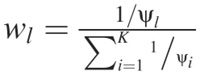 . The rationale for the KNN imputation is that the reference genes closest to the target gene are also the most informative, since the missing values in the target gene are more likely to behave similarly to that of the reference genes. Thus, when strong local correlation exists between genes in the data, KNN imputation performs well. A serious drawback of the KNN imputation using the Euclidean distance is that it does not consider negative correlations between data, which can lead to estimation error (18). Although the KNN method is very simple, it does give very good imputation results, as several comparative studies have shown (12,19).
SVD imputation
In contrast to the KNN imputation which utilizes local pairwise information between genes in the gene expression matrix, SVD imputation attempts to utilize the global information in the entire matrix in predicting the missing values. The basic concept is to find the dominant components summarizing the entire matrix and then to predict the missing values in the target genes by regressing against the dominant components. If we perform SVD to matrix Y, we get the following equation.
| 2 |
Let L = min{M,N}, matrix VT now contains L eigengenes vl (0 < l < L), and matrix U contains L eigenarrays ul (0 < l < L) (11). In the algorithm SVDimpute, the k most significant eigengenes from VT are selected, and missing value Yi,j is estimated by first regressing the expression profile vector of gene i against the K eigengenes and then using the coefficients of the regression to reconstruct from a linear combination of the K eigengenes (12). If we denote the expression profile vector of gene i in Y as y and assume that vl (l = 1,2, … , K) are the eigengenes, and are vectors that are obtained by deleting the jth component of vl and y, then the missing component Yi j is estimated as follows.
| 3 |
Since SVD can only be performed on complete matrices, the iterative expectation maximization method is used. SVDimpute performs best when global structure exists in the expression data.
Least square imputation
Recently, a family of least square optimal imputation method has been proposed (13). One of them, called LSimpute_gene, is based on the K most correlated genes. To estimate the missing value Yi,j, LSimpute_gene first selects the K most correlated genes xl (l = 1,2, … , K) in Y whose expression profiles are similar to gene i except for the jth component and with the jth component available. Then an estimate of the missing value is obtained from the reference gene xl using the single regression model. Finally, the K estimates are linearly combined to form the final estimate using empirically chosen correlation-based weight. LSimpute_gene performs best when the data has a strong local correlation structure, owing to the use of linear regression and a weighting based on correlation.
Bø et al. (13) also presents a method called LSimpute_array, for estimating missing values from array correlations using a multiple regression model. Furthermore, Bø et al. (13) presents two methods for estimating missing values by taking into consideration the estimates from LSimpute_gene and LSimpute_array. Among all these methods, LSimpute_adaptive is the best performing one, which uses an adaptive weighting scheme taking the data correlation structure into consideration to determine an appropriate weighting.
The rationale behind our approach
By taking into account the available information in the data as well as any biologically relevant domain knowledge, we would expect a better imputation result. To achieve this goal, there are two things to consider: (i) the identification of all relevant information to be used in the imputation, and (ii) a flexible computational framework for utilizing this information.
For (i), we have identified three categories of information that are useful for the imputation problem. They are information between genes (between rows of the data matrix), information between arrays (between columns of the data matrix) and biological constraints.
Almost all existing algorithms utilize the information between genes for missing value imputation. We have seen that this gene-wise information can be classified as local (in the sense that only a small subset of ‘closest’ genes in the expression matrix are taken into consideration) or global (in the sense that all genes in the expression matrix are taken into consideration). The work of (12) and our own experience showed that local information (as in KNNimpute or LSimpute) is much preferred over global information (as in SVDimpute). The imputation results from SVDimpute are generally inferior to those from KNNimpute or LSimpute. This observation agrees with our results in gene expression clustering (20), where typically only a small number of genes are in a cluster and are strongly correlated (i.e. co-expressed). We attempt to suggest a biological explanation here. We suspect that this may be a consequence of the characteristics of the gene co-expression network. It has been shown by Agrawal (21) and Noort et al. (22) that the gene co-expression network is a small world and scale free network. In such a network, there could be a large number of nodes but the network is sparse in the sense that the average number of links per node is typically much less than the total number of nodes, and there are many nodes with few connections and a small (but significant) number of nodes with many interactions. Hence, in such a network, localized co-expressions between genes are much more abundant. Arnone and Davidson (23) believe genes are influenced on average by no more than eight to ten other genes.
Information between columns (i.e. samples or time points) of the gene expression matrix can provide useful information for imputation. For temporal gene expression data, samples from adjacent time points are highly correlated. The decorrelation of the eigenarrays suggests the possibility that some of the eigenarrays represent independent cellular states. Alter et al. (11) have inferred that an eigenarray represents a state across all genes. Hence, by capturing this global array-wise correlation in the imputation, more accurate estimation should be obtainable.
One biological constraint we can make use of is the phenomenon of synchronization loss in the gene expression experiment. Cyclic systems, such as the cell cycle (24) and circadian clock (25), play a key role in many biological processes. Microarray experiments that study these systems are usually carried out by synchronizing a population of cells. Synchronization is achieved by first arresting cells at a specific biological life point and then releasing cells from the arrest so that all cells are at the same point when the experiment begins (24,26).
However, even if cells are synchronized perfectly at the beginning of the experiment, they do not remain synchronized forever (17). For example, yeast cells seem to remain relatively synchronized for two cycles (24) while wild type human cells lose their synchronization very early (27) or halfway through the first cycle depending on the arresting method. This causes the peak expression value to be lower in the second cycle and the lowest expression value to be higher for most cycling genes. A typical gene expression profile with synchronization loss is given in Figure 1.
Figure 1.

The gene expression profile of Smc3 in Spellman et al.'s experiment. The synchronization loss is significant (17).
Owing to this phenomenon, we find that the average signal power in successive cycles decreases significantly. Table 1 shows our statistical results of four datasets in Spellman et al.'s experiment. In constructing Table 1, we need to know the period of the corresponding cell cycle. However, in some microarray experiments, this may not be available. This problem can be circumvented by the following heuristic. As noted by Bar-Joseph et al. (17), synchronization loss is a continuous process. So if we compute our statistics on a fixed-length time interval and as long as that interval is long enough, synchronization loss will become obvious.
Table 1.
The statistical result of synchronization loss for four datasets in Spellman et al.'s experiment
| Dataset | No. of sampling points | No. of complete genes | Average signal energy for first cycle | Average signal energy for second cycle |
|---|---|---|---|---|
| CDC28 | 17 | 1383 | 352.78 | 288.73 |
| CDC15 | 24 | 4381 | 846.28 | 834.57 |
| Alpha factor | 18 | 4489 | 474.58 | 306.24 |
| Elutriation | 14 | 5766 | 898.48 | 435.32 |
Note that since the signal of Elutriation is available only for one cycle, we compare the average signal energy for first-half cycle and the second-half cycle.
Obviously, the three classes of information discussed earlier are not mutually independent. For example, the profiles of a set of similar genes would also give information about the correlation between sample points in the profiles. This observation is also noted in (14), where they showed that the local least square formulations of gene-wise and array-wise information are actually the same. To make efficient use of the available information (possibly highly redundant) in a coherent manner, we need a convenient and flexible computation framework. Hence, we have adopted the POCS framework for recovering loss information from existing and prior information about the data.
POCS FOR INFORMATION RECOVERY
The POCS provides a convenient framework to allow multiple pieces of prior information of different nature to be utilized to get an optimal solution. It has found many applications in many fields (28–35). The main idea of POCS is to transform every piece of a priori knowledge into a corresponding convex set and then use a convergence-guaranteed iterative procedure to search for a solution in the intersection of these sets (i.e. the solution satisfies all the a priori knowledge).
In the POCS method, every known a priori property about the original signal is formulated as a corresponding convex set in a Hilbert space H (28,36). Given m closed convex sets , and non-empty intersection , the successive projections onto the convex sets,
| 4 |
will converge to a point in the intersection C0 for any initial a0, where an is the estimate of the signal at iteration n, and Pi is the projector onto Ci defined by the following equation:
| 5 |
and is the relaxation parameter. is often used for simplicity. Figure 2a depicts the POCS framework.
Figure 2.

The POCS algorithm: (a) iterations in sequential projections for a consistent problem, in which the intersection set C0 is non-empty, (b) iterations in simultaneous projections for an inconsistent problem, in which the intersection set is empty.
When the sets are not intersecting, i.e. C0 is empty, the POCS framework can still be used with slight modification. The modified framework is called simultaneous projections, and Equation 4 is substituted by the following equation.
| 6 |
where wl are the weights on the projections satisfying and for all l. With , Equation 6 can be simplified as follows.
| 7 |
The simultaneous projections converge weakly to a point such that a weighted set-distance function is minimized (36). The situation is illustrated in Figure 2b.
The POCS method provides a very flexible framework to incorporate all a priori information to get an optimal solution. Regardless of whether it is a consistent or inconsistent problem, the convergence of the algorithm is guaranteed. For gene expression data, which is noisy and with imprecise prior information, this tolerance to imprecision is very important.
Another useful feature of the POCS algorithm is its adaptivity in finding a good solution. This can be explained as follow. Suppose we have correlation information between genes and between samples, and these two pieces of information are modeled as two convex sets Cu and Cv, respectively. In one dataset, the first piece of information may be more reliable than the second. In another dataset, it may be the opposite. This situation is depicted in Figure 3. When the information is more reliable, the corresponding convex set will be smaller in range. Since POCS always converge to the intersection, the final solution will always be dominated by the smaller set, while still satisfying the constraint imposed by the less reliable set. In this manner, a good solution that makes a wise trade-off between different prior information can be obtained.
Figure 3.

POCS adaptivity: (a) in a data dominated by gene-wise correlation, the final solution is dominated by Cu and (b) in a data dominated by array-wise correlation, the final solution is dominated by Cv.
THE POCS-BASED IMPUTATION ALGORITHM
The POCS method requires the specification of convex sets that incorporate the a priori constraints about the solution. We propose convex sets here to capture gene-wise correlation, array-wise correlation, and known biological constraint based on the rationale in The rationale behind our approach section.
Capturing gene-wise correlation
In gene expression data, genes that have close biological function would express similarly. In general, only a small subset of genes would co-express similarly and using a subset of genes for missing values estimation often results in good performance (5,13,14). To capture this localized gene-wise correlation in the gene expression data, we construct a convex set based on local least square regression as in (13) as follows. First, we select the K-most correlated genes in Y whose expression profile vectors are similar to gene i except the jth component and with the jth component available. Then we estimate the missing value in the target gene using each reference gene based on the single regression model. If we denote the expression profile vector of the target gene as y, for a reference gene x, we have
| 8 |
where e is some random noise. The factors α and β are estimated by the following equations.
| 9 |
where
and
Thus the least squares estimate of a variable f given a variable t can be written as and the variance of the residual error is given by the following equation.
| 10 |
Since we have K reference genes, we can obtain K estimates with variance of the estimation error as τl (l = 1, 2, … , K) for a missing value. A weighted average of the estimates and the corresponding variance of the estimation error are computed by the following equation.
| 11 |
| 12 |
Here we use
Bø et al. (13) propose to use
However we observed that the former definition can provide better performance in most of the experiments we conducted. Defining the positions in matrix Y of all missing values as set I, we can get an estimate , for every missing value using the above regression. Considering the possible estimation error in this method, we obtain a set as follows.
| 13 |
The projection Pu onto convex set Cu is then given by the following equation.
| 14 |
Capturing array-wise correlation
We use the PCA approach to capture the global array-wise variation. In this approach, the dominant array-wise variation of the entire dataset is summarized by a few principle components, which can be viewed as representing independent cellular states across all genes (11).
Assume we have a complete data matrix with no missing value. PCA represents the variation of each array vector y as a linear combination of principle axis vector ul (0 < l < K):
 |
15 |
The linear coefficients xl (0 < l < K) are called factor scores and ɛ denotes the residual error. For each ul, there is a corresponding eigenvalue λl. For gene expression data, eigenvalue λl indicates the relative significance of the lth eigenarray in terms of the fraction of the overall expression they captured. In PCA for gene expression data, only the K (0 < K < L) most significant eigenarray are used (10). The other L–K eigenarray are treated as noise and the signal-to-noise ratio (SNR) is given by the following equation:
| 16 |
The estimation error is given by ɛ. As in Equation 3, when a solution for a missing value is found using this method, a more reliable estimate is that the missing value lies in an interval , where τ is a parameter determined statistically [refer to Ref. (37)]. Defining the positions of all missing values in matrix Y as a set I, we can construct a convex set as follows:
| 17 |
where the is the estimated missing value using the eigenarrays, and and . The projection onto set Cv is then given by the following equation:
| 18 |
Capturing the phenomenon of synchronization loss
We propose here a series of convex sets to take advantage of the phenomenon of synchronization loss. Define the positions in matrix Y of all missing values belonging to the ith period as a set Ii, and the positions of all observed values belonging to the ith period as a set Ωi. Let function u(I) be the cardinal number of set I. We get the equation
| 19 |
with and i = 1, … , n denotes the number of periods considered.The convex set in Equation 19 has a simple geometrical structure (Figure 4). If we arrange the Y(l) (l ∈ Ii) into a vector x, it can be rewritten as follows:
| 20 |
In other word, set C now becomes a constraint on the vector length.
Figure 4.

In Rn, the constraint set Ci represents a hyperspherical surface that is centered at the origin.
The projection of an arbitrary Y(i, j) onto the set Ci is then given by the following equation:
| 21 |
It was pointed out by Kim et al. (14) that the local least square formulation of gene-wise and array-wise information is actually the same. So one may question the necessity of having the gene-wise convex set and the array-wise convex set. However, in our algorithm the two sets are constructed differently. Hence, they are not exactly equivalent, although their information may overlap significantly. We remark that the redundancy in information between the two sets does not pose a problem for our algorithm since the POCS framework can handle the redundancy, without biasing the final solution (28).
With the convex sets defined, the set theoretic estimation yields the following missing values imputation algorithm:
Select a initial estimation Y0.
For k = 1,2, … , compute Yk from Yk = w1Pu(Yk−1)+ w2Pv(Yk−1)+ w3P1 … Pn(Yk−1), where Pu,Pv,P1, … , Pn denote the projectors onto the constraint sets Cu,Cv,C1 … Cn, respectively, and w1, w2 and w3 are weighting parameters of POCS with and for all l = 1,2,3. A convenient choice is to let wl's be equal.
If , exit the iteration, else go to Step (ii).
In the above procedure, it is necessary to find a good initial point. The solution of the POCS algorithm often converges to a point in the intersection of all sets and with the least distance to the initial point. When the average value of a gene is used as the initial point for missing value estimation, the solution is the one with the least variance among all solutions which satisfy all a priori knowledge. So we propose to use the average of the gene expression profile as the initial point for our algorithm. Actually, we have also tested our algorithm with other initial point, such as zero or spline interpolation values. From the experiment results, we found that the effect of initial point is trivial.
We remark that imputation method that takes into consideration the gene and array correlation simultaneously to obtain an estimate is not a new one and has been proposed by Bø et al. (13) where they present two algorithms to use weighted averages of the estimate from LSimpute_gene and LSimpute_array. Nevertheless, POCSimpute uses a different mechanism to combine the estimates from gene correlation and array correlation. If we do not consider the cyclic loss model, the main difference between POCSimpute and LSimpute_adaptive can be concluded as follows: LSimpute_adaptive is a weighted average of the estimates from LSimpute_gene and LSimpute_array. However, POCSimpute is the nonlinear combination of two corresponding sub-algorithms (sets Cu and Cv). As indicated in Figure 2, when two convex sets are inconsistent, the estimate is the weighted average where a weighted set-distance function is minimized. When two convex sets overlaps (i.e. consistent), the estimate is a point in the intersection, which is often a point closest to the initial value used. Therefore, in POCSimpute, the estimates are weighted averages of two sub-algorithms for some missing values (the inconsistent constraints). For other missing values, the estimates are nonlinear combination from two constraint sets (the consistent constraints). POCSimpute provides a framework to adaptively select the preferred combination method. Weighted average of two estimates used in LSimpute does not necessarily produce a solution in the intersection set even if the constraint sets representing the prior knowledge overlap. Thus, POCSimpute can provide the optimal solution for all prior knowledge available while simple weighted average of different estimates may not produce the optimal solution.
EXPERIMENTAL EVALUATION
In this section, we apply our method to several microarray data sets. The first one is the study of yeast cell cycle from Spellman et al. (24) (http://cellcycle-www.stanford.edu). It contains expression profiles for 6178 genes under different experimental conditions, i.e. cdc15, and cdc28, alpha factor and elutriation experiments. In addition, one of the time series datasets contains less apparent noise than the other. Another time series data set is from (38), we denote it as fkh1_fkh2. We have also tested our algorithm on two non-time series datasets. One is the study of response to environmental changes in yeast from (26), which contains 173 samples and 6159 genes for each sample. The other is hereditary breast cancer (39). It contains 24 breast tumor samples from 21 breast cancer patients and 3226 genes are used for each tumor sample.
Each dataset is pre-processed for evaluation by removing rows containing missing expression values, yielding ‘complete’ matrices. The missing value estimation techniques are then tested by randomly removing data values and then computing the estimation error. In the experiments, between 1 and 15% of the values is removed from each dataset. The normalized root mean square (NRMS) error is calculated as follows.
| 22 |
where Y is the original gene expression matrix and is the estimation obtained by the missing value imputation algorithm.
To assess the performance of our missing value estimation algorithm, we also compare the NRMS error of our algorithm with the KNNimpute, SVDimpute and LSimpute_adaptive algorithms. It would be interesting to investigate how much is gained in imputation accuracy using the cyclic loss model. So we also test our method without using the cyclic loss model and it is denoted as POCSnoncyclic. For KNNimpute and LSimpute_adaptive methods, we choose K = 10, i.e. we use the 10 closest genes as the reference genes. The rationale for this is that Troyanskaya et al. (12) observes that the best result of KNNimpute is obtained when K is in the range 10–20 and Bø et al. (13) proposes using K = 10 for LSimpute. For SVDimpute method, 20% of the eigengenes are selected for regression, as proposed by Troyanskaya et al. (12). In our algorithm, there are two parameters: the number of genes used as neighbors in set Cu and the number of eigenarrays used in set Cv. We find that using 10 genes as neighbors for set Cu and 20% of the eigenarrays for set Cv is a good choice for the microarray data sets tested.
In the proposed algorithm, the parameter τ that is associated with both Cu and Cv are determined statistically as described in (37) and in most cases, τ should be a small value. In our experiments, we find that the performance of our algorithm has no dramatic change for τ ∈ [0.01,0.3] although a smaller value is preferred. For simplicity, we set τ = 0.1 in all experiments.
The performance of our algorithm is evaluated in Figures 5–8 for all time series and non-time series datasets. In each of the data sets and at each level of missing values, 15 Monte Carlo simulations are performed with independent selections of missing entries. The same test data with identical entries missing are used for all imputation algorithms and the average of the performance indices is regarded as the final result. In the figures, the horizontal axis denotes the name of the dataset. The vertical axis denotes the NRMS value. We can say that our algorithm can achieve significantly less error than the KNNimpute, SVDimpute and LSimpute_adaptive methods.
Figure 5.

Estimation performance (NRMS) by KNNimpute, SVDimpute, LSimpute_adaptive, POCSimpute without cyclic loss model and POCSimpute for 1% missing values.
Figure 8.

Estimation performance (NRMS) by KNNimpute, SVDimpute, LSimpute_adaptive, POCSimpute without cyclic loss model and POCSimpute for 15% missing values.
A further illustration of the improved accuracy of POCSimpute is given in Figure 9, which shows the histograms for the distribution of the RMS errors. The test data is Elutriation with 4489 genes and 18 arrays and 5% missing values. We find that POCSimpute has the narrowest error distribution, i.e. there are very few large imputation errors compared to the KNNimpute and LSimpute_adaptive.
Figure 9.

Error histograms of different estimation methods and 5% data missing rate for the Elutriation dataset: (upper) the KNNimpute, (middle) the LSimpute_adaptive and (lower) the POCSimpute.
Although the error histogram can give us an idea of how the imputation errors are distributed, we may also be interested to see how the imputation algorithms perform as a function of the actual expression level. The box and whisker plots of the estimation errors relative to the true expression values (log2 expression ratio) in the range are provided in Figure 10. The box depicts the median, the upper and lower quartiles of the error distribution. The test data is Elutriation with 4489 genes and 18 arrays and 5% missing values. From the plots, we can find some interesting properties of our estimation. When the magnitude of true values is small, the performances of the three methods are close. However our algorithm has lower error median and spread when true expression values are medium or large (log2 ratio of between 0.68 and 1.5). A possible reason causing this is that when we construct the set Cv to capture the array-wise correlation, we use SNR instead of noise variance (we use the noise variance in set Cu). SNR is a ratio and it allows Cv to change adaptively with the magnitude of the estimated missing values (or true values). In a microarray experiment, the expression ratios of those genes with medium or high expression levels are considered to be more reliable and hence are taken with greater faith. If those values are missing due to experimental artifacts or contaminations, we would like them to be more reliably imputed as well. Our algorithm seems to provide a better estimate for missing values whose true values have medium or large magnitudes.
Figure 10.

Box and whisker plots of the estimation errors relative to the true values in the range: (upper) KNNimpute, (middle) LSimpute_adaptive and (lower) POCSimpute.
DISCUSSION AND CONCLUSION
In the microarray missing value estimation problem, we often have different a priori knowledge about the missing value for different experiments and different genes. By utilizing all available information about the missing values into their estimation, the optimal result can be obtained. In this paper, we propose a set theoretic approach based on POCS which we call POCSimpute for the problem of microarray missing value estimation. POCSimpute can adaptively find an optimal solution regardless of whether the global or local correlation structure is dominant in the target data. Furthermore, it can conveniently make use of biological constraints to get a better estimate. Experiments show that our algorithm can achieve a significant reduction of error compared to some available algorithms.
Even though POCSimpute shows good performances in our experiments, our algorithm also has some shortcomings. First, it is an iterative algorithm and has higher computation cost than SVDimpute and LSimpute_gene. However, for imputation purposes, better estimation accuracy always has higher priority than speed (18). In our experiments, for a microarray data with 4381genes and 24 arrays and 10% missing values, it requires 2–3 min on a computer with 2.00 GHz CPU and 512 MB RAM using MATLAB. We think that the time cost of our algorithm is still acceptable for most experiments. Second, in POCSimpute, the sets which make use of the phenomenon of synchronization loss work best for time series data. We hope that some other sets using more general biological properties can be found in the future. Nevertheless, we think that the POCS framework introduced here opens up a convenient way for incorporating other biological constraints that one can conceive of. If one can find convex sets with strong biological meanings, the estimated values would then be biologically even more relevant.
It is also important to point out here that we should avoid skewing the estimate when using a priori knowledge for estimation. To achieve this goal, we should follow two general guidelines. First, the a priori information we used should be well established and proven to be appropriate. The a priori information frequently used in estimation problem is discussed by Stark and Yang (28) and Combettes (36). Second, when we construct a convex set based on the a priori knowledge, good modeling method is important. Modeling of the reliability of convex sets for medical image reconstruction is discussed by Yan (30). Soft projections and regularizations can be used to solve a number of problems due to overlapping and missing data and nonintersecting convex sets (30). In the situation where some a priori knowledge does not fit the data perfectly, we should ensure that the corresponding convex set does not skew or degrade the estimate. For example, the convex sets based on cyclic loss property in this paper are used for time series microarray dataset. In a dataset without cyclic loss phenomenon, ϕi in Equation 19 will generally be equal. The corresponding convex sets then degenerate to the requirement that the average power of all observed values and all missing values are equal. Fortunately, this is a reasonable assumption in microarray data and it would not skew our estimate. In fact, we observed that this has contributed to the slight improvement for the non-cyclic datasets (Figures 5–8) even though the cyclic loss model does not really apply in these cases.
Figure 6.

Estimation performance (NRMS) by KNNimpute, SVDimpute, LSimpute_adaptive, POCSimpute without cyclic loss model and POCSimpute for 5% missing values.
Figure 7.

Estimation performance (NRMS) by KNNimpute, SVDimpute, LSimpute_adaptive, POCSimpute without cyclic loss model and POCSimpute for 10% missing values.
Acknowledgments
This work is supported by a CityU interdisciplinary grant (project 9010003), a CityU strategic research grant (project 7001706) and a grant from the Hong Kong Research Grant Council (project CityU122005). Funding to pay the Open Access publication charges for this article was provided by the Hong Kong Research Grant Council (project CityU122005).
Conflict of interest statement. None declared.
REFERENCES
- 1.Armstrong S.A., Staunton J.E., Silverman L.B., Pieters R., den Boer M.L., Minder M.D., Sallan S.E., Lander E.S., Golub T.R., Korsmeyer S.J. MLL translocations specify a distinct gene expression profile that distinguishes a unique leukemia. Nature Genet. 2002;30:41–47. doi: 10.1038/ng765. [DOI] [PubMed] [Google Scholar]
- 2.Muro S., Takemasa I., Oba S., Matoba R., Ueno N., Maruyama C., Yamashita R., Sekimoto M., Yamamoto H., Nakamori S., et al. Identification of expressed genes linked to malignancy of human colorectal carcinoma by parameteric clustering of quantitative expression data. Genome Biol. 2003;4:R21. doi: 10.1186/gb-2003-4-3-r21. [DOI] [PMC free article] [PubMed] [Google Scholar]
- 3.Kim S., Dougherty E.R., Chen Y., Sivakumar K., Meltzer P., Trent J.M., Bittner M. Multivariate measurement of gene expression relationships. Genomics. 2000;67:201–209. doi: 10.1006/geno.2000.6241. [DOI] [PubMed] [Google Scholar]
- 4.Duggan D.J., Bittner M., Chen Y., Meltzer P., Trent J.M. Expression profiling using cDNA microarrays. Nature Genet. 1999;21:10–14. doi: 10.1038/4434. [DOI] [PubMed] [Google Scholar]
- 5.Ouyang M., Welsh W.J., Georgopoulos P. Gaussian mixture clustering and imputation of microarray data. Bioinformatics. 2004;20:917–923. doi: 10.1093/bioinformatics/bth007. [DOI] [PubMed] [Google Scholar]
- 6.Yang Y.H., Buckley M.J., Dudoit S., Speed T.P. Technical Report 584. UC Berkeley: Department of Statistics; 2000. Comparison of methods for image Analysis in cDNA microarray data. [Google Scholar]
- 7.Eisen M.B., Spellman P.T., Brown P.O., Botstein D. Cluster analysis and display of genome-wide expression patterns. Proc. Natl Acad. Sci. USA. 1998;95:14863–14868. doi: 10.1073/pnas.95.25.14863. [DOI] [PMC free article] [PubMed] [Google Scholar]
- 8.Brown M.P., Grundy W.N., Lin D., Cristianini N., Sugnet C.W., Furney T.S., Ares M.J., Haussler D. Knowledge-based analysis of microarray gene expression data by using support vector machines. Proc. Natl Acad. Sci. USA. 2000;97:262–267. doi: 10.1073/pnas.97.1.262. [DOI] [PMC free article] [PubMed] [Google Scholar]
- 9.Oba S., Sato M., Takemasa I., Monden M., Matsubara K., Ishii S. A Bayesian missing values estimation method for gene expression profile data. Bioinformatics. 2003;19:2088–2096. doi: 10.1093/bioinformatics/btg287. [DOI] [PubMed] [Google Scholar]
- 10.Raychaudhuri S., Stuart J.M., Altman R.B. Principal components analysis to summarize microarray experiments: application to sporulation time series. Pac. Symp. Biocomput. 2000:455–466. doi: 10.1142/9789814447331_0043. [DOI] [PMC free article] [PubMed] [Google Scholar]
- 11.Alter O., Brown P.O., Botstein D. Singular value decomposition for genome-wide expression data processing and modeling. Proc. Natl Acad. Sci. USA. 2000;97:10101–10106. doi: 10.1073/pnas.97.18.10101. [DOI] [PMC free article] [PubMed] [Google Scholar]
- 12.Troyanskaya O., Cantor M., Sherlock G., Brown P., Hastie T., Tibshirani R., Botstein D., Altman R.B. Missing values estimation methods for DNA microarrays. Bioinformatics. 2001;17:520–525. doi: 10.1093/bioinformatics/17.6.520. [DOI] [PubMed] [Google Scholar]
- 13.Bø T.H., Dysvik B., Jonassen I. LSimpute: accurate estimation of missing values in microarray data with least squares method. Nucleic Acids Res. 2004;32:e34. doi: 10.1093/nar/gnh026. [DOI] [PMC free article] [PubMed] [Google Scholar]
- 14.Kim H., Golub G.H., Park H. Missing value estimation for DNA microarray gene expression data: local least squares imputation. Bioinformatics. 2005;21:187–198. doi: 10.1093/bioinformatics/bth499. [DOI] [PubMed] [Google Scholar]
- 15.Bar-Joseph Z., Gerber G.K., Gifford D.K., Jaakkola T.S., Simon I. Continuous representations of time-series gene expression data. J. Comput. Biol. 2003;10:341–356. doi: 10.1089/10665270360688057. [DOI] [PubMed] [Google Scholar]
- 16.Gan X.C., Liew A.W.C., Yan H. Missing value estimation for microarray data based on projection onto convex sets method. In Proceedings of International Conference on Pattern Recognition (ICPR2004); Cambridge, UK, III. 2004. pp. 782–785. [Google Scholar]
- 17.Bar-Joseph Z., Farkash S., Gifford D.K., Simon I., Rosenfeld R. Deconvolving cell cycle expression data with complementary information. Bioinformatics. 2004;20:i23–i30. doi: 10.1093/bioinformatics/bth915. [DOI] [PubMed] [Google Scholar]
- 18.Sehgal M.S.B., Gondal I., Dooley L.S. Collateral missing value imputation: a new robust missing value estimation algorithm for microarray data. Bioinformatics. 2005;21:2417–2423. doi: 10.1093/bioinformatics/bti345. [DOI] [PubMed] [Google Scholar]
- 19.Nguyen D.V., Wang N., Carroll R.J. Evaluation of missing value estimation for microarray data. J. Data Sci. 2004;2:347–370. [Google Scholar]
- 20.Wu S., Liew A.W.C., Yan H. Cluster analysis of gene expression data based on self-splitting and merging competitive learning. IEEE Trans. Inf. Technol. Biomed. 2004;8:5–15. doi: 10.1109/titb.2004.824724. [DOI] [PubMed] [Google Scholar]
- 21.Agrawal H. Extreme self-organization in networks constructed from gene expression data. Phys. Rev. Lett. 2002;89:268702. doi: 10.1103/PhysRevLett.89.268702. [DOI] [PubMed] [Google Scholar]
- 22.Noort V.V., Snel B., Huynen M. The yeast coexpression network has a small-world, scale-free architecture and can be explained by a simple model. EMBO Rep. 2004;5:280–284. doi: 10.1038/sj.embor.7400090. [DOI] [PMC free article] [PubMed] [Google Scholar]
- 23.Arnone A., Davidson B. The hardwiring of development: organization and function of genomic regulatory systems. Development. 1997;124:1851–1864. doi: 10.1242/dev.124.10.1851. [DOI] [PubMed] [Google Scholar]
- 24.Spellman P.T., Sherlock G., Zhang M.Q., Iyer V.R., Anders K., Eisen M.B., Brown P.O., Botstein D., Futcher B. Comprehensive identification of cell cycle-regulated genes of the yeast Saccharomyces cerevisiae by microarray hybridization. Mol. Biol. Cell. 1998;9:3273–3297. doi: 10.1091/mbc.9.12.3273. [DOI] [PMC free article] [PubMed] [Google Scholar]
- 25.Panda S., Antoch M.P., Miller B.H., Su A.I., Schook A.B., Straume M., Schultz P.G., Kay S.A., Takahashi J.S., Hogenesch J.B. Coordinated transcription of key pathways in the mouse by the circadian clock. Cell. 2002;109:307–320. doi: 10.1016/s0092-8674(02)00722-5. [DOI] [PubMed] [Google Scholar]
- 26.Gasch A.P., Spellman P.T., Kao C.M., Carmel-Harel O., Eisen M.B., Storz G., Botstein D., Brown P.O. Genomic expression programs in the response of yeast cells to environmental changes. Mol. Biol. Cell. 2000;11:4241–4257. doi: 10.1091/mbc.11.12.4241. [DOI] [PMC free article] [PubMed] [Google Scholar]
- 27.Shedden K., Cooper S. Analysis of cell-cycle-specific gene expression in human cells as determined by microarrays and double-thymidine block synchronization. Proc. Natl Acad. Sci. USA. 2002;99:4379–4384. doi: 10.1073/pnas.062569899. [DOI] [PMC free article] [PubMed] [Google Scholar]
- 28.Stark H., Yang Y. Vector Space Projections, A Numerical Approach to Signal and Image Processing, Neural Nets, and Optics. NY: John Wiley & Sons; 1998. [Google Scholar]
- 29.Hedley M., Yan H., Rosenfeld D. An improved algorithm for 2D translational motion artifact correction. IEEE Trans. Med. Imaging. 1991;10:548–553. doi: 10.1109/42.108589. [DOI] [PubMed] [Google Scholar]
- 30.Yan H. Signal Processing in Magnetic Resonance Imaging and Spectroscopy. NY: Marcel Dekker Inc.; 2002. [Google Scholar]
- 31.Weerasinghe C., Liew A.W.C., Yan H. Artifact reduction in compressed images based on region homogeneity constraints using projection on to convex sets algorithm. IEEE Trans. Circuits Syst. Video Technol. 2002;12:891–897. [Google Scholar]
- 32.Gan X.C., Liew A.W.C., Yan H. A smoothness constraint set based on local statistics of BDCT coefficients for image postprocessing. J. Image Vision Computing. 2005;23:731–737. [Google Scholar]
- 33.Yan H., Mao J. The relation of the low frequency restoration methods to the Gerchberg–Papoulis Algorithm. Magn. Reson. Med. 1990;16:166–172. doi: 10.1002/mrm.1910160116. [DOI] [PubMed] [Google Scholar]
- 34.Liew A.W.C., Yan H. An adaptive spatial fuzzy clustering algorithm for 3D MR image segmentation. IEEE Trans. Med. Imaging. 2003;22:1063–1075. doi: 10.1109/TMI.2003.816956. [DOI] [PubMed] [Google Scholar]
- 35.Gan X.C., Liew A.W.C., Yan H. Blocking artifact reduction in compressed images based on edge-adaptive quadrangle meshes. J. Visual Commun. Image Rep. 2003;14:492–507. [Google Scholar]
- 36.Combettes P.L. The foundation of set theoretic estimation. Proc. IEEE. 1993;81:182–208. [Google Scholar]
- 37.Park S.H., Kim D.S. Theory of projection onto the narrow quantization constraint set and its application. IEEE Trans. Image Process. 1999;8:1361–1373. doi: 10.1109/83.791962. [DOI] [PubMed] [Google Scholar]
- 38.DeRisi J.L., Iyer V.R., Brown P.O. Exploring the metabolic and genetic control of gene expression on a genomic scale. Science. 1997;278:680–686. doi: 10.1126/science.278.5338.680. [DOI] [PubMed] [Google Scholar]
- 39.Hedenfalk I., Duggan D., Chen Y., Radmacher M., Bittner M., Simon R., Meltzer P., Gusterson B., Esteller M., Kallioniemi O.P., et al. Gene-expression profiles in hereditary breast cancer. N Engl. J. Med. 2001;344:539–549. doi: 10.1056/NEJM200102223440801. [DOI] [PubMed] [Google Scholar]