

Abstract
A method that considerably reduces the computational and memory complexities associated with the generation of high dimensional (≥3) feature maps for image segmentation is described. The method is based on the K-nearest neighbor (KNN) classification and consists of two parts: preprocessing of feature space and fast KNN. This technique is implemented on a PC and applied for generating three-and four-dimensional feature maps for segmenting MR brain images of multiple sclerosis patients.
Keywords: Multispectral segmentation, MRI, Feature space, Feature map, KNN classification
I. INTRODUCTION
Magnetic resonance imaging (MRI) with its superb soft tissue contrast is an ideal modality for investigating central nervous system disorders. Quantitative estimation of tissue volumes provides important information about the natural progression of disease and helps to objectively evaluate the efficacy of therapeutic intervention. The multi-model nature of MRI allows the implementation of multi-spectral techniques for quantitative estimation of tissue volumes. Feature map-based classification techniques are attractive for segmenting MR images because they are fast, simple to implement, and allow fusion of expert’s input in tissue classification.9,13,26,4 The quality of segmentation generally improves with dimensionality of the feature space if multi-spectral images are available. However, in practice feature map analysis is most commonly limited to two-dimensions and rarely to three dimensions.26,4,1,7 Full exploitation of MR images with multiple contrasts for accurate classification of heterogeneous pathology may require higher dimensional (≥3) feature space analysis. In practice, generation of feature maps in higher dimensional feature space poses severe problems because of the increased memory requirements and the associated computational complexity.9,13,26 For example, in the case of four dimensional feature space with dynamic intensity range of [0, 255], the total size of the feature space is (256)4=4GB. Such large data size is extremely difficult to handle on PC’s and conventional workstations. In this study, a method that allows the generation of high dimensional feature maps on a PC is presented. This method is applied to segment brain images of multiple sclerosis (MS) patients that were acquired using three and four echoes.4
The two commonly used statistical classifiers for feature map generation are Parzen Window and K Nearest Neighbor (KNN) schemes.13,26 Both these classifiers are nonparametric in nature and use selected seeds as the training set. A number of studies have demonstrated the superiority of KNN over the Parzen Window method.8,25 Therefore, in these studies we utilized the KNN technique. However, the proposed method is equally applicable to the Parzen Window technique with appropriate modifications.
It’s well known that KNN method is computationally expensive because it requires the calculations of distance.26 Therefore a number of fast KNN methods have been developed during the last 40 years. Of these fast methods, the branch and bound12,18,21,17,19 and k-distance transformation (K-DT) based algorithms26,11,10 have a number of attractive features. The K-DT based algorithm is efficient, but has extensive memory requirements. On the other hand, the branch and bound algorithm is less efficient, but has moderate memory requirements. Warfield et al.26 employed Borgefors’s chamfer DT 6 in 2D, and Ragnelmam’s quasi-Euclidean corner EDT 23 in higher dimensions. However, in addition to the memory problems in high dimensions, the multiple scans in high-dimensional feature space and a large amount of sorting operations also require heavy computational power.11 Cuisenaire11,10 was able to considerably reduce the computational load at the expense of memory requirements since the dynamic structure used to implement the bucket sorting algorithm requires allocation of memory in chunks rather than element by element. Therefore, it is not feasible to directly apply any of these algorithms to high dimensional feature space. This perhaps explains lack of studies on the application of K-DT based KNN methods for feature map with dimension greater than 3.26,7,11,24
In the current studies we developed and applied an efficient and novel method based on the “divide and conquer” approach for generating the high dimensional feature maps. In this method, the whole feature space was partitioned into subdivisions to deal with the memory problem. In addition, a pre-classification procedure was adopted for reducing the number of points in the feature space that need to be classified with the fast KNN algorithm. This considerably reduces the computational complexity. Subsequently, a modified K-DT based algorithm was developed for implementing the fast KNN method in high dimensional feature space for the classification of all remaining unclassified feature vectors.
II. FEATURE SPACE PARTITION
The memory requirements dramatically increase with the dimensionality of the feature space. Partitioning the feature space eliminates this problem and a simple way to accomplish this is to divide the feature space into hypercubes. The feature vectors in each hypercube can be classified separately and thus reduce the memory requirements. This can be understood using a 2D case, without loss of generality, as demonstrated in Fig. 1. The entire 2D feature space is shown in Fig. 1(a). The feature space can be divided in to smaller squares as shown in Fig. 1(b) and each square represents one subdivision or subspace (here we define subspace to be synonymous with subdivision and not space with reduced dimensions) in the feature space. In image segmentation using KNN, usually an effective distance, distE, for each seed in the feature space is assumed. The classification of feature vectors beyond distE is not affected by that seed.26,11 The classification of one subspace would be affected by the training seed prototypes inside that subspace and those around that subspace within distE. Therefore to determine the classification of one subspace, that subspace needs to be expanded to incorporate all the training seed prototypes involved in the classification of that subspace. In order to accomplish this, the whole feature space and the seed prototypes are virtually shifted by distE along each dimension to form the overlap between subdivisions as shown in Fig. 1(c). In this figure, the subdivisions, indicated by the solid line, represent the original subspace, while each dashed square surrounding the small solid square represents the subspace expanded by distE along each dimension. Once feature space is partitioned into subspaces as shown in Fig. 1(c), same classification algorithm can be used separately on each single subspace surrounded by the dashed area. In Fig. 1(d), the feature vector (solid dot) inside the solid square can be classified by the training seed points contained within the circle of radius distE that is centered on the feature vector. On the other hand, for classification of the feature vectors that are close to the boundary of the subspace, we need to examine the seed points outside the solid square (Fig. 1(d)), but confined within the overlapping region. This procedure is repeated for each subspace (or solid square in Fig. 1(c)) until the whole feature space is classified. This substantially reduces the data size that needs to be processed simultaneously. For example, in the case of 4D feature space with a dynamic range of [0, 255] that is subdivided into (4)4=256 subspaces, the classification can be performed on each subspace of size (64)4=16MB.
FIGURE 1.

Schematic representation of the 2D feature space. (a) Whole feature space inside the solid line, (b) division of feature space into subspaces, (c) seed prototypes inside the overlapping dashed line regions that affect the boundaries of a subspace, (d) dashed square representing the region that needs to be included for classification of feature vectors inside one subspace. The solid dots represent the feature vectors.
III. REDUCTION OF FEATURE VECTORS TO BE CLASSIFIED IN FEATURE SPACE
The next step is to simplify the computational complexity of KNN by recognizing the feature vectors either as tissues or as null feature vector before applying the fast KNN algorithm. This is accomplished by using the following three rules:
Detect the number of seed prototypes within the circle of radius distE that is centered on a feature vector. Discard the feature vector if the number of seed points in this circle is smaller than K.
If the number of seed prototypes within the circle is equal to K and if the number of seed points belonging to the same class is > K/2, then the feature vector is automatically assigned to this class (winner takes all).
Within the circle, if the number of points, K′, is greater than K but the sum of seeds (excluding the winner) of the other classes is less than K/2, the class is automatically determined to be the same as the winner.
Use of these three rules does not involve any comparison of distances and therefore can considerably accelerate the computations. The application of these three rules to feature space is elaborated below.
Since the seed prototype has limited effective distance, distE, there is no need to use KNN to classify the whole feature space. In fact, according to the above rules, only those points in the feature space that have at least K effective seed prototypes need to be classified using KNN. Since the whole feature space is divided, we will concentrate on one of the subspaces. To this end, an efficient method that can be employed in a batch mode for determining the number of seed prototypes for the classification of one feature vector is proposed. Using circles, each of radius distE, centered on each of the seed prototypes (seed prototypes are indicated using small solid circles in Fig. 2(a)), we can determine the feature vectors that need to be classified by retaining those which are contained within the solid square and covered by at least K circles according to the rule 1 above. This concept is described in Fig. 2(a) which shows three seed prototypes in three small circles. In this figure, “1” represents the region covered by only single circle, “2” denotes the overlapping region covered by two circles, and “3” denotes the region of intersection of all the three circles. If K equals to 1, then the region to be classified will be all those points in the (sub) feature space with a value of at least 1. If K equals 2, then the region to be classified will be all those points with a value of at least 2. In this way, the number of feature vectors to be classified is considerably reduced. Rules 2 and 3 are applied to those feature vectors that still remain unclassified after applying rule 1. If there are exactly K circles that cover this feature vector, then the feature vector can be automatically classified by counting the number in each class of those seed prototypes and assigning it to the same class as the majority of the seed prototypes (that can be easily realized by counting the number of seeds in each class inside the circle centered on the feature vector with radius of distE). If there are K′> K circles cover the feature vector to be classified, the feature vector is assigned to the same class as those seeds that are at least (K′-K/2) in number; otherwise it is kept as unclassified that needs be further classified later using the fast KNN method. These operations can be repeated for each subspace. Finally, after the application of these rules, the feature vectors in the whole feature space that still need to be classified are restricted to those located at the interface (unclassified region in Fig. 2(b)).
FIGURE 2.

(a) Procedures for reducing the number of feature vectors for KNN classification in one subspace. Seed prototypes are shown as solid small circles. (b) The unclassified feature vectors in the entire feature space are restricted to the interfaces between the classes.
Assuming that there are C classes, and the dimensions of the D-dimensional subspace are dim(1),…,dim(D), the algorithm can be coded as follow:
Code for pre-processing of each subspace
Denote subspace as sfs, allocating C arrays of the same size of sfs;
Input: distE, k, all seeds affect the classification of sfs, a hyper-ball with radius of distE and value of 1.
Output: The partially classified feature space.
If no seeds affect the classification (or effective seeds < k) of sfs then
Indicate sfs as indentified;
skip all;
Else do:
For each seed do:
Centralizing the hyper-ball on the seed;
If the seed belong to class c then array c is added with the hyper-ball;
sfs always added with the hyper-ball;
Find out feature vectors in sfs of value = K (denote as efv);
Find the max value of the C arrays at efv;
Assign the classes of efv according to the class of the max;
Find out feature vectors in sfs of value > K (denote as gfv);
Find the max value of the C arrays at gfv (denote as mv);
Find out where(mv - (sfs(gfv)-ceil(K /2))) > 0 (denote as gmv)
Assign the classes of gmv according to the class of the max;
End.
Obviously, storing the subspace separately would be beneficial in the subsequent processing. Repetition of the above code on all subspaces is very fast. For feature space of 2564, under IDL (Interactive Data Language) environment 16, it usually takes 1–2 minutes for a few hundred seeds in all the cases we tested.
IV. CLASSIFICATION USING FAST KNN
As indicated above, the only remaining feature vectors that still need to be classified are those located at the interface of classes (unclassified region in Fig. 2(b)). Thus the only seed prototypes that need to be considered are those located in the region that is expanded by distE in the unclassified regions (regions confined within dashed line in Fig. 3). Therefore not only the feature space that needs to be scanned for classification is greatly reduced but the seed prototypes involved in the classification are also reduced. This considerably reduces the complexity of the KNN classification. At this stage one could use either branch and bound method or K-DT based fast KNN methods12,26 or their variants.
FIGURE 3.

Regions showing the seed prototypes that need to be taken into consideration.
When using the branch and bound method to classify the feature vectors, the efficiency can be improved by striking a balance between the branches and the seeds within terminal nodes. The strategy on whether to work on the whole feature space or subspaces depends on the distribution of the unclassified points. It is preferable to work on the whole space if the unclassified points are concentrated in a relatively small feature space. Otherwise, the strategy of subspace is preferred. In case of K-DT based method, it is preferred to work on subspaces.
In these studies we developed a new algorithm based on the K-DT methods similar to those proposed elsewhere.26,11 The first step in this new algorithm is to retain all the seeds that would have an effect on the classification of unidentified feature vectors. For each subspace that contains the unidentified feature vectors, we count the number of seeds for each class in this subspace, and form a compact representation of the location of the unidentified feature vectors as a list in which the location are mapped to consecutive numbers. This helps generate a compact histogram in terms of the locations of the unidentified feature vector (see the algorithm below). The algorithm involves an allocation of a pointer array of size of (number of classes, distE+1). Complete the following loop for distEE running from 0 to distE: load in hyper-hollow-ball with an outer radius of distEE and an inner radius of (distEE−1); for each seed involved in the classification, center the hyper-hollow-ball on the seed, and find the locations of the feature vectors inside the hyper-hollow-ball, then push those locations into the pointer with indices (class of seed, distEE), and repeat this procedure for all the seeds. After that, for each class, we can use the compact representation of the unidentified feature vectors to map the locations in the corresponding pointer into representation of consecutive numbers, and end the distEE loop. The last step in the classification involves operations based on the histograms of those consecutive numbers. With an array HistSum of size [number of classes of cluster × number of unclassified feature vectors], following loop is performed: for distEE equal 0 to distE, for each class, make a cumulative sum of the histogram of the those corresponding numbers to the corresponding element of the array HistSum for distEE. The classification is completed by first finding if there is feature vector with sum value of HistSum over all classes at distEE greater or equal K, and determine which class is of the max value. The feature vector is classified as the same class of the max, thus eliminating the classified feature vector from the waiting list. The procedure will be repeated until all unclassified feature vectors are determined.
The algorithm can be coded as:
Code of fast KNN
Input: unclassified feature vectors (denote as ufv) in subspace,
Seeds involved in classification,
K value, distE, hyper-hollow-balls with outer radia from 0 to distE and inner radia one less than the outer radia;
Output: classification of feature vectors;
Forming a list to map the location of ufv into consecutive number (denote as fs_list_map) (this compact form is adopted for using histogram);
Allocating a array of size of (classes,number of ufvs ) (denote as h_array);
Allocate a pointer array of size of (number of classes, distE+1) (denote as p_array);
For distEE equal 0 to distE do:
Load hyper-hollow-ball with radius of distEE;
For each seed do:
Centralizing the hyper-hollow-ball on the seed;
Find out the locations of ufvs inside the ball;
Push the locations into *p_array(class of seed, distEE);
For each class i do:
Using fs_list_map to map *p_array(i, distEE) into numbers (denote as compact_location(i, distEE));
h_array(i,:)= h_array(i,:)+histogram(compact_location(i,distEE));
finding the maximum of sum over i in h_array;
if there are items greater or equal to K then:
find out the max over i in h_array;
assign the corresponding ufv to the class of the max;
eliminating the classified ufv from ufv in h_array;
End.
The above code is repeated for all the subspaces with unclassified feature vectors. One of the advantages of the above algorithm is that the hyper-hollow-ball can be computed separately which provides the flexibility of choosing different definitions for the distance metric (chessboard, city block, Euclidian etc.).15
V. METHODS
As an example, the above method was applied to generate three- and four-dimensional feature maps for segmenting the MR brain images of multiple sclerosis (MS) patients that were acquired as a part of our ongoing studies. All MR images were acquired on a 1.5 T, General Electric scanner. A quadrature birdcage resonator was used for radio frequency transmission and signal reception. For four dimensional feature map generation, MR images were acquired using the AFFIRMATIVE pulse sequence.5 The total number of slices was 42 (3 mm thick, contiguous and interleaved) covering the brain from vertex to foramen magnum. The other acquisition parameters were: repetition time, TR, of 16,000 ms, field-of-view 240 mm x 240 mm, 256 x 256 image matrix. The total acquisition time for all the 42 slices was 16 minutes. The total number of patients for this part of the study was 12. The AFFIRMATIVE pulse sequence is based on the fast spin echo sequence (FSE) and produces four images per each slice location. The first two images are the fast spin echo images acquired at echo times (TE) of 17 ms and 102 ms. The last two images are acquired at these two echo times, but incorporate an off resonance pulse for generating magnetization transfer contrast and an inversion pulse for suppressing cerebrospinal fluid (CSF). These four images provide differing tissue contrasts and are used for generating the four-dimensional feature maps.
For the generation of three dimensional feature maps, dual echo FSE and Fluid Attenuation Inversion Recovery (FLAIR) MR images acquired on a separate group of 45 MS patients, using the same hardware. The FSE images were acquired with TR = 6800 ms, TE1/TE2 = 12 ms/86 ms. The FLAIR images were acquired with TR = 10002 ms, TI (inversion recovery time) = 2200 ms and TE = 91 ms. The total number of patients in this part of the study was 20. The other parameters (slice thickness, field-of-view, image matrix) were identical to those used for the acquisition of the AFFIRMATIVE images.
Image Segmentation
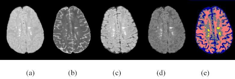
Prior to performing the segmentation using feature map, images were pre-processed that include registration (required for aligning FSE images with FLAIR images), bias correction, anisotropic diffusion filtration, stripping of the extrameningeal tissues, and histogram standardization. Image registration was performed using the global optimization of mutual information.14 The four AFFIRMATIVE images were acquired in an interleaved fashion within a given TR and do not require any registration. Bias correction was applied for minimizing the radio frequency inhomogeneities introduced by the coil using the procedure described elsewhere.3 Images were filtered using the anisotropic diffusion filter27 for reducing the noise with minimal image blurring. A semi-automatic method was developed for stripping the extramenigeal tissues. Finally, image intensities were standardized through histogram mapping.22,20 Results of these image preprocessing operations for the FLAIR and the FSE images are shown in Fig. 4–8. Same preprocessing operations (with the exception of registration) were also performed on the AFFIRMATIVE images.
FIGURE 4.
Registration of FLAIR and short TE FSE images, (a) FLAIR image before registration, (b) FLAIR image after registration, (c) target image (short echo FSE, also referred to as the proton density (PD)) .
FIGURE 8.

FSE and FLAIR images prior to (top row) and following (bottom row) histogram standardization.
Prior to generating the feature maps, seed points were selected from a subset of images by an experienced neurologist and neuroradiologist. A set of visualization tools were developed to help the experts select the seed points. These visualization tools were also helpful in the choice of proper DistE, k, and number of seeds. Since only 2D and 3D feature vectors (seeds) and feature maps can be directly viewed on the monitor, these visualization tools are restricted to the 2D or 3D feature space. Figures 9 and 10 show the screen dumps of the 2D and 3D visualization tools, respectively. As can be seen from these figures, the visualization tools allow display the images of any slice, selection and editing of seed points (eliminating individual seed from the set of seeds), and display feature vectors and feature maps. It is not easy to develop comparable visualization tools when the dimensionality of the feature space exceeds 3, however, we use tools of Fig. 10 to view various 3D (sub) data sets for the higher dimensional data to gain some insight into the distributions of seeds. In this case it is difficult to edit the seeds and view the feature maps. In the case of 4D feature space, we determine DistE, k, and the number of seeds based on the experience gained with the 2D and 3D analysis. Since the seeds are more sparsely distributed in higher dimensional space even when the number of seeds increases, we used smaller k and larger DistE when the dimension exceeded 3.
FIGURE 9.

Visualization tool for 2D application. First column is image viewer for seeds pick up, second column is feature map and seeds viewer, and third column is seeds editor.
FIGURE 10.
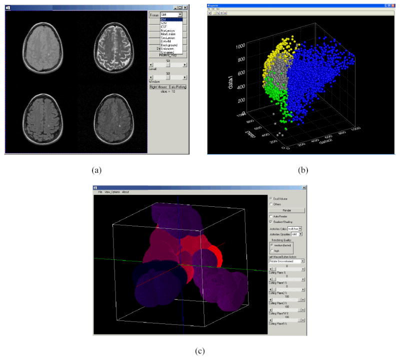
Visualization tool for 3D application. (a) Image viewer, analyzer and seeds pick up, (b) seeds viewer and editor, (c) feature map viewer.
Because of the histogram standardization of all the images, the same feature map that is generated from the training data set can be used for segmenting all the images acquired with the same protocol. Since this feature map generation algorithm deals with subspaces, multiple look up tables (the sub feature maps) that relate the image intensity to the address of each subspace were generated and only those subspaces with nonempty feature map were used. In these studies, for 168 AFFIRMATIVE images (4 echoes and 42 slices, each slice with a size of 256×256), when the normalized feature space was divided into (4)4=256 subspaces, it took 1~2 minutes on a PC for completing the feature map based segmentation. For the FSE and FLAIR images, segmentation of 126 images (3 echoes and 42 slices, each slice with a size of 256×256) was completed within one minute on a PC.
VI. RESULTS AND CONCLUSIONS
Figures 11(a)–(d) show the four AFFIRMATIVE brain MR images of same location of an MS subject. The first two images ((a) and (b)) correspond to the FSE images with short and long TE values respectively. The corresponding images with the off resonance and the inversion pulses turned on are shown in (c) and (d). The differing tissue contrasts can be appreciated on these images. The feature maps derived from the AFFIRMATIVE training data set of MS brains are shown in Fig. 12. This figure shows several sections of the 4D feature maps for one of the 256 subdivisions of the original feature space. In this figure D1–D4 represent dimension 1 to dimension 4 of the 4D subdivision of the feature space. In these maps, the brightest and gray color areas represent white and gray matter respectively, while the dark gray and black colors indicate unclassified and unused regions respectively. Figure 12(a) shows the feature maps generated before applying the fast KNN algorithm, and Fig. 12(b) shows the corresponding maps after the application of the fast KNN algorithm. As can be seen from these figures, the application of the fast KNN algorithm has classified all the previously unclassified feature vectors.
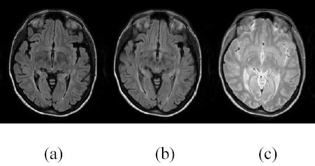
FIGURE 11.
(a)-(d): Four AFFIRMATIVE images. (e): segmented image using 4D feature map.
FIGURE 12.
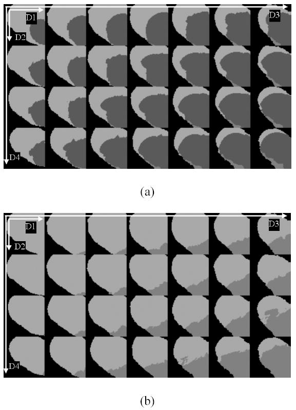
Sections of 4D feature maps of one subspace, (a) is generated before applying the fast KNN algorithm, and (b) is after applying the fast KNN algorithm.
Finally the segmented image based on the above feature maps is shown in Fig. 11(e). In this segmented image, gray matter, white matter, CSF and lesion regions are shown in gray, pink, blue, and yellow colors respectively. The excellent classification of the tissues can be easily appreciated in this figure, especially the merit on identification of MS lesions.
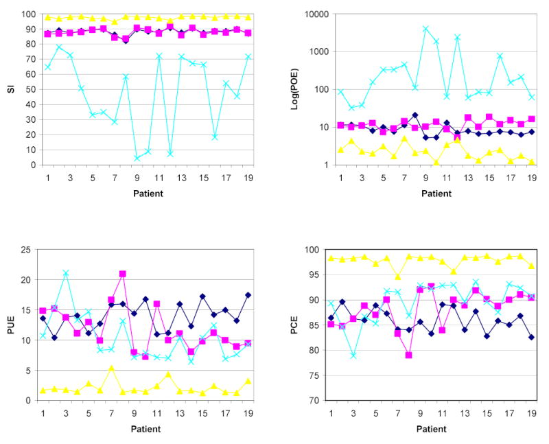
There is no gold standard against which the segmentation results generated with the high dimensional feature maps on human brains can be compared. In the absence of such gold standard, we relied on the tissue classification results provided by experts. For a quantitative evaluation, we compared the tissue volumes (Seg) based on the segmentation of the 12 MS brains using the four-dimensional feature maps with the reference volumes (Ref) generated by the experts by computing the four quantitative measures defined in Eqs. (1)–(4).2 In these equations POE, PUE, PCE refer to the over-, under-, and the correctly estimated percentage of tissue volumes, respectively and SI is the similarity index. Of the 12 patients, images of one patient were used for generating the training data set. The parameters used for generating the feature map were: feature space dimensions of 256×256×256×256, distE = 40, total number of seeds = 10,030 (3,000 for CSF, 3,000 for gray matter, 3,000 for white matter, and 1,030 for lesions), and K = 9. The results on rest of the 11 patients are given in Fig. 13. Different ordinate scales are used in these graphs in order to clearly visualize the variations in each metric. The total time used for generating the feature maps, including the preprocessing steps, is around 3 hours using interactive data language (IDL) on PC.
FIGURE 13.

Quantitative analyses of 4D segmentation of AFFIRMATIVE images. The symbols diamond, square, triangle, and cross represent gray matter, white matter, CSF, and lesion respectively.
| (1) |
| (2) |
| (3) |
| (4) |
As an example, the two FSE and FLAIR images on one MS patient are shown in Fig. 14 along with the segmentation results, based on the three-dimensional feature maps. In the segmented images, gray matter, white matter, CSF and lesion are shown in gray, white, blue, and red respectively. The parameters used for generating the feature maps were: feature space is 1024×1024×1024, distE = 120, total number of seeds = 7,000 (2,000 for CSF, 2,000 for gray matter, 2,000 for white matter, and 1,000 for MS lesion), and K = 11. Results of the quantitative analysis on the 19 patients (one patient data set was used for generating the training set) are shown in Fig. 15. Different ordinate scales are used in these graphs in order to clearly visualize the variations in each metric. The time taken for generating the feature map, including the preprocessing, was around 5 hours using IDL on PC.
FIGURE 14.

Segmentation on FLAIR+FSE.
FIGURE 15.
Quantitative analyses of 3D segmentation of FSE+FLAIR images. The symbols diamond, square, triangle, and cross represent gray matter, white matter, CSF, and lesion respectively.
Based on these various measure, particularly the percentage of correct identification, as reflected by high PCE values, the performance of the segmentation results based on both three- and four-dimensional feature maps appear very satisfactory. A few observations can be made, based on the results shown in Fig. 13 and 15. Overall, the four-dimensional map generates better segmentation of gray- and white-matter than the 3-dimensional map. In three cases (Patient 07, Patient 10 and Patient 11) the SI values are lower in four-dimensional case than in the three-dimensional case, partly because of the poor image contrast seen in these AFFIRMATIVE image sets. The segmentation of CSF is comparable in both the cases. Results on the MS lesions are inferior to that observed in the other three tissues. This is mainly due to the presence of a small number of false positives. Since the lesion volumes are small, even small false classifications would exaggerate the similarity measure, and subsequently augment the POE. Clearly more work is needed in automatic identification and elimination of the false lesion classifications. While difficult to quantify, both the experts that manually classified the tissues have strongly felt that the three- and four-dimensional techniques have resulted in significantly improved tissue classifications compared to segmentation based the two-dimensional feature maps that we have been routinely using on our patient population. There is still room for improving the performance of the segmentation by tuning the parameters such as the number of seeds, K values, effective distance distE, etc. Improvements in the pre-processing steps, such as the method proposed in28, would enhance the quality of segmentation.
In conclusion, a method for generating the feature map in high dimensional feature space is proposed and implemented. The method is based on the divide and conquer concept and the classification of feature space is based on the K-DT algorithm. The division of the feature space into multiple subdivisions allowed getting around the memory problems. Computational efficiency of the KNN is further improved by reducing the number of points to be classified and developing a fast KNN algorithm. This technique is implemented on a PC for generating three- and four-dimensional feature maps for segmenting MR brain images of multiple sclerosis patients. Results of the segmentation are quantitatively compared with the manual classification performed by experts.
FIGURE 5.

FSE and FLAIR images prior to (top row) and following (bottom row) bias correction.
FIGURE 6.

FSE and FLAIR images prior to (top row) and following stripping (bottom row).
FIGURE 7.

FSE and FLAIR images prior to (top row) and following (bottom row) filtration.
Acknowledgments
This work is supported by the National Institutes of Health grant R01 EB02095. We thank Dr. Jerry Wolinsky for providing access to the images on the MS patients and the validated AFFIRMATIVE data sets and identifying the training seeds used for generating the feature maps. We also thank Dr. Rakesh Gupta for performing the manual classification, based on the FSE and FLAIR images. We acknowledge Dr. Sushmita Datta for developing part of the analysis software and Ms. Meghana Mehta for her help with segmentation.
References
- 1.Amato U, Larobina M, Antoniadis A, Alfano B. Segmentation of magnetic resonance brain images through discriminant analysis. J Neurosci Methods. 2003;131(1–2):65–74. doi: 10.1016/s0165-0270(03)00237-1. [DOI] [PubMed] [Google Scholar]
- 2.Anbeek P, Vincken KL, van Osch MJP, Bisschops RHC, Grond J. Probabilistic segmentation of white matter lesions in MR imaging. NeuroImage. 2004;21:1037–1044. doi: 10.1016/j.neuroimage.2003.10.012. [DOI] [PubMed] [Google Scholar]
- 3.Ashburner, J.. Another MRI Bias Correction Approach. The 8th International Conference on Functional Mapping of the Human Brain, Sendai, Japan, June 2–6, 2002. Available on CD-Rom, also appeared in NeuroImage, 16(Suppl. No. 2).
- 4.Bedell BJ, Narayana PA. Volumetric analysis of white matter, gray matter, and CSF using fractional volume analysis. Magn Reson Med. 1998;39:961–969. doi: 10.1002/mrm.1910390614. [DOI] [PubMed] [Google Scholar]
- 5.Bedell BJ, Narayana PA, Wolinsky JS. A dual approach for minimizing false lesions classifications on magnetic resonance images. Magn Reson Med. 1997;37:94–102. doi: 10.1002/mrm.1910370114. [DOI] [PubMed] [Google Scholar]
- 6.Borgefors G. Distance transformation in arbitrary dimensions. Computer Vision, Graphics, and Image Processing. 1984;27:321–145. [Google Scholar]
- 7.Cárdenes R, Warfield SK, Macìas E, Santana JA, Ruiz-Alzola J. An Efficient Algorithm for Multiple Sclerosis Lesion Segmentation from Brain MRI. In Franz R. Pichler Roberto Moreno-Dìaz, editor. Computer Aided Systems Theory - EUROCAST. 2003;2003:542–551. [Google Scholar]
- 8.Clarke LP, Velthuizen RP, Phuphanich S, Schellenberg JD, Arrington JA, Silbiger M. MRI: Stability of Three Supervised Segmentation Techniques. Magnetic Resonance Imaging. 1993;11:95–106. doi: 10.1016/0730-725x(93)90417-c. [DOI] [PubMed] [Google Scholar]
- 9.Cline HE, Lorenson WE, Kikinis R, Jolesz F. Three-Dimensional Segmentation of MR Images of the Head Using Probability and Connectivity. Journal of Computer Assisted Tomography. 1990;14(6):1037–1045. doi: 10.1097/00004728-199011000-00041. [DOI] [PubMed] [Google Scholar]
- 10.Cuisenaire, O. and B. Macq. Fast k-NN classification with an optimal k-distance transformation algorithm. Proc. 10th European Signal Processing Conference (EUSIPCO), pp. 1365–1368, September, 2000.
- 11.Cuisenaire, O.. Distance transformations: fast algorithms and applications to medical image processing, Thèse présentée en vue de l’obtention du grade de Docteur en Sciences Appliquées, UCL/TELE, Louvain-la-Neuve, Octobre 1999.
- 12.Fukunaga K, Narendra P. A branch and bound algorithm for k-nearest neighbors. IEEE Transactions on Computers. 1975;24:750–753. [Google Scholar]
- 13.Gerig, G., J. Martin, R. Kikinis, O. Kübler, M. Shenton, and F. Jolesz. Automatic segmentation of dual-echo MR head data. Proc 12th Int. Conf. on Information Processing in Medicine Imaging, Wye U.K., July, 1991, 175–187, Springer Berlin, 1991.
- 14.He R, Narayana PA. Global optimization of mutual information: Application to three-dimensional retrospective registration of magnetic resonance images. Comp Med Imag Graph. 2002;(26)(4):277–292. doi: 10.1016/s0895-6111(02)00019-8. [DOI] [PubMed] [Google Scholar]
- 15.http://www.mathworks.com/access/helpdesk/help/toolbox/images/morph15.html
- 16.http://www.rsinc.com/
- 17.Jiang Q, Zhang W. An improved method for finding nearest neighbors. Pattern Recognition Letters. 1993;14:531–535. [Google Scholar]
- 18.Kamgar-Parsi B, Kanal LN. An improved branch and bound algorithm fro computing k-nearest neighbours. Pattern Recognition Letters. 1985;3:7–12. [Google Scholar]
- 19.Kim BS, Park SB. A fast K nearest neighbor finding algorithm based on the ordered partition. IEEE Trans PAMI. 1986;8:761–766. doi: 10.1109/tpami.1986.4767859. [DOI] [PubMed] [Google Scholar]
- 20.Meier DS, Guttmann CRG. Time-series analysis of MRI intensity pattern in multiple sclerosis. NeuroImage. 2003;20:1193–1209. doi: 10.1016/S1053-8119(03)00354-9. [DOI] [PubMed] [Google Scholar]
- 21.Niemann H, Goppert R. An efficient branch-and-bound nearest neighbor classifier. Pattern Recognition Letters. 1988;7:67–72. [Google Scholar]
- 22.Nyul LG, Udupa JK, Zhang X. New variants of a method of MRI scale standardization. IEEE Trans Med Imag. 2000;19(2):143–150. doi: 10.1109/42.836373. [DOI] [PubMed] [Google Scholar]
- 23.Ragnelmam I. The euclidean distance transformation in arbitrary dimensions. Pattern Recognition Letters. 1993;14:883–888. [Google Scholar]
- 24.Romero, E., Jean-Marc Raymackers, B. Macq and O. Cuisenaire. Automatic fibrosis quantification using a k-NN classificatory. 23rd Annual International Conference of the IEEE Engineering in Medicine and Biology Society (EMBC 2001), Istanbul, October 25–28, 2001.
- 25.Vaidyanathan RP, Clarke LP, Velthuizen RP, Phuphanich S, Hall LO, Bezdek JC. Comparison of supervised MRI segmentation methods for tumor volume determination during therapy. Magn Reson Imaging. 1996;13(5):719–728. doi: 10.1016/0730-725x(95)00012-6. [DOI] [PubMed] [Google Scholar]
- 26.Warfield SK. Fast k-NN classification for multichannel image data. Pattern Recognition Letter. 1996;17:713–721. [Google Scholar]
- 27.Weickert, J.. Anisotropic Diffusion in Image Processing. Teubner, Stuttgart, 1998.
- 28.Weisenfeld, N. I. and S. K. Warfield. Normalization of joint image-intensity statistics in MRI using the Kullback-Leibler divergence. Preprint, IEEE ISBI, 2004.