Strategies in probabilistic categorization: Results from a new way of analyzing performance

Abstract

The “Weather Prediction” task is a widely used task for investigating probabilistic category learning, in which various cues are probabilistically (but not perfectly) predictive of class membership. This means that a given combination of cues sometimes belongs to one class and sometimes to another. Prior studies showed that subjects can improve their performance with training, and that there is considerable individual variation in the strategies subjects use to approach this task. Here, we discuss a recently introduced analysis of probabilistic categorization, which attempts to identify the strategy followed by a participant. Monte Carlo simulations show that the analysis can, indeed, reliably identify such a strategy if it is used, and can identify switches from one strategy to another. Analysis of data from normal young adults shows that the fitted strategy can predict subsequent responses. Moreover, learning is shown to be highly nonlinear in probabilistic categorization. Analysis of performance of patients with dense memory impairments due to hippocampal damage shows that although these patients can change strategies, they are as likely to fall back to an inferior strategy as to move to more optimal ones.

In the last decade or so, probabilistic category learning tasks, in which various cues are probabilistically (but not perfectly) predictive of class membership, have become more and more popular. They have given insight into implicit forms of learning, cognitive flexibility, and the use of feedback signals in the brain. The tasks have also been used to elucidate cognitive deficits in several patient populations, including patients with medial temporal lobe damage and patients with Parkinson’s disease (Knowlton et al. 1994, 1996; Hopkins et al. 2004; Shohamy et al. 2004). Moreover, in fMRI studies, probabilistic categorization has been shown to rely on several areas involved in memory, with interesting suggestions as to how these areas might work together (Poldrack et al. 2001; Aron et al. 2004; Rodriguez et al. 2006).

While probabilistic categorization has thus proven its utility in cognitive neuroscience research, it is still unknown exactly how people solve such tasks. It could be that participants attempt to find an abstract rule underlying the category assignments. Alternatively, repeated exposure to exemplars could slowly lead to a tendency for subjects to group similar stimuli in the same categories (an “information integration” approach in the terminology of Ashby et al. 1998). Subjects could even simply memorize an answer for each individual cue combination, independent of any abstract rules or learned categories. There are thus a potentially large number of strategies and variants by which a subject could approach this task and achieve significantly better-than-chance performance.

Unfortunately, it is very difficult to infer from a categorizer’s performance on the task in which way he or she is solving it. This conundrum is made more difficult by the way in which probabilistic category learning data are usually analyzed, which is to calculate the proportion of optimal responses over the course of the experiment. Recently, Gluck et al. (2002) introduced a richer way of analyzing performance. They recognized that responses of participants to particular stimuli may fall into consistent patterns that are informative about the way that participants approach the task. They called the patterns in performance “strategies.” Most participants in their study could be identified as using one such strategy, and Gluck et al. (2002) were also able to show a progression, throughout 200 trials, from simple strategies to more complex ones.

Here, we present an extension and elaboration of the strategy analysis introduced by Gluck et al. (2002). This new version is based on maximum likelihood estimation and has several advantages over the previous, simpler analysis. First, it allows analysis of individual behavior on a trial-by-trial basis, which, in turn, makes it possible to identify “switch points” at which a participant stops responding according to one strategy and begins responding in a new way. It also allows us to compare participant performance against a benchmark of “random” performance.

In the sections below, we first introduce the general methodology of the new strategy analysis. Then, we tackle three more general questions with respect to these analyses: (1) Can they work in principle? (2) Do they work in practice? (3) Can they offer a new perspective on probabilistic categorization? To answer the first question, we present Monte Carlo simulations showing that both strategies and strategy switches can be identified in simulated data from a probabilistic categorization task (Experiment 1). To answer the other two questions, we apply the analyses to existing data sets from human categorizers. In Experiment 2, we show that the analyses offer a new perspective on learning, and that they can predict responses of categorizers. In Experiment 3, we show how the analyses can shed new light on the difference between normal participants and a patient population.

Basics of strategy analysis

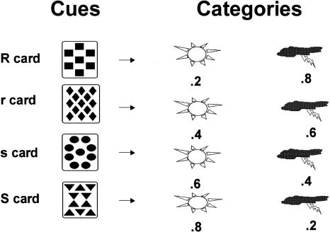
The task analyzed in this paper is the Weather Prediction task (Knowlton et al. 1994). In this task, participants are told that they will have to predict whether there will be sun or rain on the basis of four cue cards. Each card predicts sun with a given likelihood: Some show that sunshine is more likely; others that rain is more likely (Fig. 1).

Figure 1.

Four cards in the Weather task, and the likelihoods with which they predict the outcomes, rain and sun. The strong rain (“R”) and sun (“S”) cards each predict the weather (rain or sun) with 80% probability, while the weaker rain (“r”) and sun (“s”) cards each predict the outcome with 60% probability. One, two, or three cards are presented on each trial, and the probability of each outcome on a given trial is a function of the probabilities of all cards present on that trial.

On any one trial, participants are presented with a pattern consisting of one, two, or three cards, and have to give a binary response (i.e., “sun” or “rain”). This response can be thought of as being based on an underlying disposition to answer “sun” or “rain” to the presented pattern with a certain probability. Since there are 14 patterns, one could represent the total disposition of the participant at any one moment as a vector v_p with 14 elements p_i, each equal to the likelihood of answering “sun” to one pattern i. The analysis we propose is an attempt to infer which disposition v_p a participant is using at any one trial in the experiment. Here, we discuss the concepts behind this analysis; mathematical details can be found in Materials and Methods.

From the one response on trial t, it is impossible to deduce the disposition of the participant toward all patterns. Even the disposition to the pattern i presented on trial t cannot be deduced (e.g., if the participant answered “sun,” only a value of p_i of 0 is ruled out; all other values are still possible). However, if the disposition of the participant remains constant over several trials, it becomes possible to identify that disposition from the pattern of responses of the participant. For example, p_i becomes more and more clear when a participant answers “sun” to every instance of pattern i in a series of trials.

Our analysis tries to capture the disposition of the participant, v_p, by fitting 11 ideal types v_s to a series of responses of the participant, with each ideal type v_s corresponding to one of the strategies. Each ideal type v_s stipulates a disposition π_s,i to each pattern i. For example, a “single-cue” strategy of answering “sun” to every pattern that contains the card with diamonds and “rain” to all other patterns, could be translated into an ideal type in which π_s,i is 1 for every pattern containing the diamonds card, and 0 for all remaining patterns.

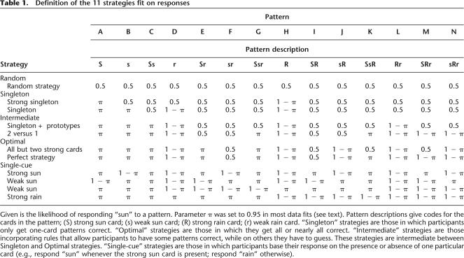
Even when participants are following a strategy, they will sometimes respond differently than the strategy prescribes because of error and exploration. The likelihood π_s,i of responding “sun” to a pattern i is therefore set not to 1 or 0, but to the scalar π or to 1 − π, with π being close to but not equal to 1.⁸ If a strategy stipulates that a participant should respond “sun” to a certain pattern i, (s)he is thus assumed to respond “sun” with likelihood π (e.g., 0.95), and “rain” with likelihood 1 − π (e.g., 0.05). π_s,i can be equal to π or 1 − π, but it can also be 0.5 if a strategy stipulates that participants respond randomly to the pattern. Table 1 defines each of the 11 strategies in terms of the likelihood of responding “sun” to each pattern. These likelihoods can be used to fit windows of trials, by allowing one to calculate the likelihood of the recorded responses given that a certain strategy is used.

Table 1.

Definition of the 11 strategies fit on responses

Given is the likelihood of responding “sun” to a pattern. Parameter π was set to 0.95 in most data fits (see text). Pattern descriptions give codes for the cards in the pattern; (S) strong sun card; (s) weak sun card; (R) strong rain card; (r) weak rain card. “Singleton” strategies are those in which participants only get one-card patterns correct. “Optimal” strategies are those in which they get all or nearly all correct. “Intermediate” strategies are those incorporating rules that allow participants to have some patterns correct, while on others they have to guess. These strategies are intermediate between Singleton and Optimal strategies. “Single-cue” strategies are those in which participants base their response on the presence or absence of one particular card (e.g., respond “sun” whenever the strong sun card is present; respond “rain” otherwise).

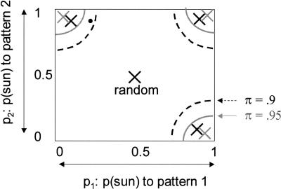
We refer to π as the “assumed consistency parameter,” as it stipulates how consistently strategies are followed. Mathematically, this parameter functions as an error tolerance criterion. With higher values of π, fewer responses that do not match a strategy are needed to reject it. This is true for all strategies except one: the so-called “random” strategy. This strategy assumes that responses are generated by “random” behavior (a 50–50 likelihood of “sun” or “rain” independent of the presented pattern). Such random behavior need not really be random; it might also be that a participant switches strategies very quickly, or responds on the basis of a probabilistic rule closer to random than to any of the strategies. Response patterns that do not closely fit any of the other strategies are usually fit best by the random strategy, as there are no real errors in this strategy: “sun” or “rain” answers fit the strategy equally well. With increasing values of π, more response patterns are fit by the random strategy. This is shown graphically in Figure 2.

Figure 2.

Each response pattern is a point in the space of all p_j values. For presentation purposes, we only show values for two patterns, 1 and 2 (with associated likelihoods of a “sun” response of p₁ and p₂). Crosses denote the ideal types of four strategies (e.g., the one in the upper left corner assumes that participants respond sun with likelihood π to pattern 1, and likelihood 1 − π to pattern 2). All response patterns within the black semicircle around each cross are best fit by the strategy exemplified by each cross if the assumed consistency parameter π is set to 0.9. All patterns not within a circle are best fit by the random strategy in the middle. Increasing π to 0.95 decreases the diameter of the circles to the gray ones, increasing the number of response patterns allocated to the random strategy. The response pattern exemplified by the little black circle would be classified as belonging to the upper left strategy with a π of 0.9, but to the random strategy with a π of 0.95. Semicircles are made up for presentational purposes. (The shape of the strategy fit regions depends not only on π but also on the number of trials fit, and on the other strategies that are fit to the response patterns.)

The analysis described above assumes that the disposition of the participant remains fairly constant over several trials. In reality, this disposition evolves over trials, as is evident from the fact that participants achieve a higher proportion of correct responses throughout training. To investigate how strategy use evolved over the course of the task, we fit our ideal-types v_s to partly overlapping windows of trials (typically, windows are 24 trials, and overlap 50%). If two subsequent windows are best fit by different strategies, we assume that a strategy switch has been made. To identify the switch, we look at how well responses are fit by both the strategy of the preceding and the following window, and estimate when this fit function shows an inflection point (an extreme point of a function’s second derivative, i.e., a point where the change of the change is maximal). If the preceding and following strategies both show an inflection point on a certain trial (or within five trials of one another), we assume that a switch has occurred on that trial.

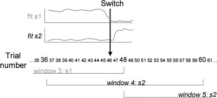
Figure 3 shows a hypothetical example in which two strategies, s₁ and s₂, are fit to a sequence of trials (the x-axis shows the trial number). Each has a certain fit to the trials, and hypothetical functions describing the fit of the two strategies on the trial sequence are shown above the trials (with higher values of the function denoting a better fit). Strategy s₁ fits best on the third window of trials (trial 25–48), but then strategy s₂ fits best on the next two windows (window 4 covering trials 37–60; and window 5, trials 49–72). Since two succeeding windows are fit best by different strategies, the analysis assumes that a switch has been made. It then tries to identify the trials on which strategies stop and start fitting. Strategy s₁ stops fitting well around trial 44, while strategy s₂ starts fitting well from trial 48 on. As the inflection points of both fit functions are close to one another in this case, the analysis places the strategy switch in the middle of the two, at trial 46.

Figure 3.

Schema showing how switch points are identified. When on one window of trials a different strategy is followed than on the next, a switch is assumed to have occurred. Here, a participant switched from strategy s₁, fitting best in the third window, to strategy s₂, fitting best in the fourth window. The derivative of the fit function of strategies s₁ and s₂ over trials is then estimated. If both show a large change close to one another (i.e., less than five trials apart), a switch is assumed to have occurred on the trial in between trials with maximal change in both derivatives. In the figure, the switch is assumed to have occurred on trial 46.

Our analysis assumes that participants, during learning, tend to make relatively discrete switches from one strategy to the next. An alternative would be that participants slowly change their disposition v_p throughout learning. We do not present evidence against this possibility, but note that all-or-none learning, with sudden breaks in performance, has been found in other domains as well (Estes 1960; Restle 1965; Gallistel et al. 2004). We return to this issue in the General Discussion.

Results

Experiment 1: Monte Carlo analyses

To validate the analysis set out above, we performed Monte Carlo simulations in which data were first generated using a certain strategy, and then fit by all strategies. This had two goals: to uncover whether the data-generating strategy would be identified by our analyses, and to investigate the influence of the parameter π, the assumed consistency parameter, on the proportion of correct strategy identifications.

First, 400 series of 24 trials were generated using a random strategy from the 11 listed in Table 1. Data generation was done in four ways, by letting simulated participants err in 0%, 2.5%, 5%, or 10% of trials against the chosen strategy. We then fit all strategies to the generated series, and identified the strategy that fit best. This was done setting π to 0.9, 0.95, 0.975, or 0.995.

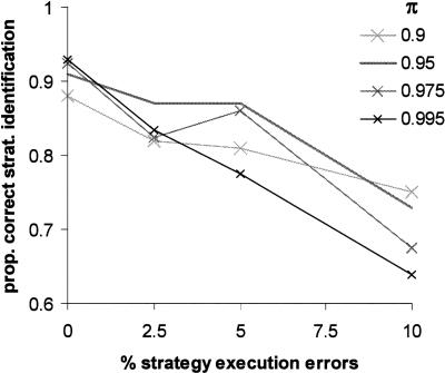
Figure 4 shows the percentage of series in which the best-fitting strategy was exactly the one that generated the data. The proportion of correct strategy identifications decreased with increasing numbers of strategy errors, from around 92%–70%, but in all conditions was far above chance. The assumed consistency parameter, π, was of less importance, with all values yielding reasonable performance. In general, lower values of π were better if many strategy execution errors were made, while higher values did better when few errors were made. This is consistent with the idea that higher values of π tolerate less deviation from the expected strategy. Fitting with a π of 0.95 yielded correct fits over the whole range of execution error percentages, and was therefore adopted in all simulations described below, and our fits of data.

Figure 4.

Results from the Monte Carlo simulations. Runs of 24 trials were simulated in which one strategy was followed with a set proportion of strategy execution errors. Given is the proportion of runs for which the followed strategy was correctly identified by the analysis, using different values for the assumed consistency parameter π. Best performance overall was reached with a value for π of 0.95.

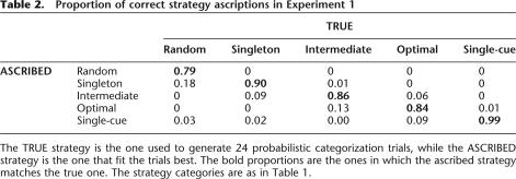
Of the errors made in the strategy analysis, most involved relatively minor mistakes, in that two similar strategies were interchanged. For example, data generated by one intermediate strategy might be misidentified as having been generated by another one. Some strategies, especially one-cue strategies in which participants base their judgment on the presence or absence of one card, were correctly identified in almost all cases (see Table 2 for a breakdown of errors for the case with 2.5% execution errors and π = 0.95).

Table 2.

Proportion of correct strategy ascriptions in Experiment 1

The TRUE strategy is the one used to generate 24 probabilistic categorization trials, while the ASCRIBED strategy is the one that fit the trials best. The bold proportions are the ones in which the ascribed strategy matches the true one. The strategy categories are as in Table 1.

Next, we looked at longer simulated trial series (40 trials, simulated with 2.5% execution errors and π set at 0.95). In this case, the percentage of strategies correctly identified went up to 92.5%, with now almost all mistakes being confusions of two minimally different strategies.

Finally, we generated a series of 96 trials, in which a switch from one strategy to another either did or did not occur somewhere between the 25th and 72nd trials. When a switch occurred, both the pre-switch and post-switch strategies were randomly chosen from Table 1 with no restriction other than that the strategies be different. We then used our analyses to identify the strategy switch point. Also for this set of simulations, simulated participants made 2.5% execution errors, while π was held constant at 0.95. Fitting all trials with one strategy, without taking the switch into account, yielded surprising results. In 52% of cases, the strategy identified over all 96 trials was neither the one followed before the switch, nor the one followed after the switch, but instead a “spurious strategy.” For example, two single-cue strategies taken together may be identified as an optimal multicue strategy. This provides another motivation for our emphasis on finding blocks of consistent strategy use. Our switch point analysis, however, was able to identify that a switch had occurred in 95% of cases. In 26% of cases, the switch was located to zero, one, or two trials from the real switch, with 17% more being diagnosed within five trials. In another 39% of cases, no switch was pinpointed, but an area of insecurity was diagnosed at the right spot (see Materials and Methods for a diagnosis of the area of insecurity). In such cases, the strategies before and after the switch were identified correctly in >80% of cases. The false alarm rate of the analysis was reasonably low: In sequences of 96 trials without a switch, false switches were found in 19% of cases.

The Monte Carlo simulations show that when a strategy is consistently followed over a block of trials, it can be identified by our analysis. The simulations also highlight a weakness of the analyses. Mixtures of strategies are not identified very well: When over the fitted series of trials two or more strategies follow each other, the resultant best fit sometimes is neither strategy but a spurious one. In analyses of empirical data we therefore kept the fitted series as short as possible, even though with shorter series the likelihood of a mistaken strategy identification increased. To counter such decreased reliability, we only ascribed a strategy to a participant if two consecutive series of trials were best fit by the same strategy.

Experiment 2: Healthy young adults

Experiment 1 showed that when a strategy is used to generate data, it can reliably be recovered by our analysis from the response data. The simulations do not speak to whether human participants, in fact, generate responses using strategies. To test this, we applied our analyses to an existing data set of healthy young adults (university students) performing the Weather task. We set out, first, to ascertain that the analysis could fit strategies to human data, and second, to determine whether strategies fit on the basis of an individual’s prior responses would be good predictors of that individual’s subsequent responses. If a fitted strategy does not predict subsequent responses, it would be a sign that the strategy is not a good descriptor of what the individual is doing or that the individual is following no fixed strategy; in either case, this would greatly lessen the utility of performing strategy analysis as a way to conceptualize human categorization behavior.

Best-fit strategies

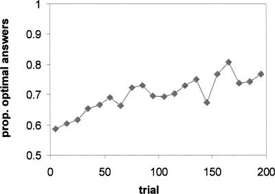
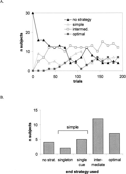
Figure 5 shows the performance of participants over the 200 trials, as originally reported in Gluck et al. (2002). From a level close to chance, performance increased to ∼80% optimal answers. Although this suggests a virtually linear increase, the strategy analyses paint a different picture. Most participants quickly acquired a strategy (see Table 3). Early in training (Fig. 6A), most participants were best fit by a single or intermediate strategy, with few or none best fit by an optimal strategy. By the end of training, however, more than half of participants were best fit by either an optimal or an intermediate strategy. Figure 6B shows how many participants were fit best by each type of strategy over the final 40 trials.

Figure 5.

Average proportion of optimal responses through 200 trials in Experiment 2.

Table 3.

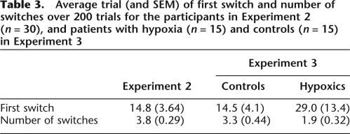
Average trial (and SEM) of first switch and number of switches over 200 trials for the participants in Experiment 2 (n = 30), and patients with hypoxia (n = 15) and controls (n = 15) in Experiment 3

Figure 6.

Strategy use. (A) Strategy use over the 200 trials. Strategies were fit over partly overlapping windows of 24 trials, which are labeled by midpoint. “Singleton strategies” and “Single Cue” strategies are collapsed into “Simple Strategies” for clarity. Other strategy groupings are as in Table 1. (B) End strategy, fit over the last 40 trials. Strategies are grouped as in Table 1.

Strategies thus became more complex during learning, but this is by no means a linear process. Although there was a clear trend from simple to complex strategies across 200 trials in the group data of Figure 6A, individual participants continued to adopt and drop strategies, sometimes dropping a complex strategy for a simpler one. Even optimal strategies were occasionally adopted, then dropped in favor of less beneficial strategies.⁹

Response prediction

If the strategies explored in the analysis (and listed in Table 1) describe the behavior of participants well, then an individual participant’s response on trial t should be predicted by the strategy fit on a window of trials preceding trial t. We used a 20-trial window to infer the strategy the subject was using leading up to trial t. Then we used Table 1 to generate the likelihood of a “sun” response to the pattern on trial t, based on the inferred strategy. We correlated the match between actual and predicted response using the Goodman-Kruskall Wallis γ-correlation.¹⁰ We also considered whether the inferred strategy was a better predictor than two others: first, the response given by the participant to the pattern on previous trials in which it was presented, and second, the outcome observed on previous trials in which the pattern was presented. In each of these two cases, we considered the prediction based on the single most recent prior presentation of the pattern, and also the prediction based on all previous trials at which the pattern was presented, weighted by distance to the current trial. Predictions were in the latter case based on a moving average. The most recent trial in which the pattern was presented had a weight of either 0.25 or 0.5, and weights of earlier trials with the pattern dropped exponentially, with the constraint that all weights add to 1. Only trials 21–200 were used in this analysis, as trial 21 was the first for which a strategy could be fit on 20 preceding trials.

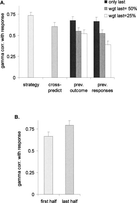
Figure 7A shows the average γ-correlation with current responses for all predictors. The fitted strategy was able to correctly predict the next response on the majority of trials (γ-correlation of nearly 0.75); γ-correlations for this approach were higher than for predictions made either on the most recent previous outcome, paired t-test [t₍₂₉₎ = 3.53, P = 0.001], or on the most recent previous response to the pattern [t₍₂₉₎ = 3.54, P = 0.001]. When the outcome and response predictions were extended to a moving average, predictions were actually less successful than considering only the most recent presentation [for the 0.5 weight, response: t₍₂₉₎ = 10.29, P < 0.001; outcome: t₍₂₉₎ = 12.66, P < 0.001].

Figure 7.

Average γ-correlation over trials 21–200 between actual responses given by participants, and predictors. (A) γ-Correlation over all trials, with as predictors the strategy fit over the previous 20 trials, the response given on the previous occurrence of the same pattern, and the outcome on the previous occurrence of the same pattern. The latter two predictors are also given in the form of moving averages, in which all previous occurrences of the same pattern are used to construct the predictor. The most recent trial counts either for 50% in the predictor, or for 25%. The predictor labeled “cross-predict” is the strategy fit on the previous 20 trials of a random other participant. (B) γ-Correlation between the prediction from the fitted strategy and the actual response, averaged over trials 21–100 (“first half”) and 101–200 (“last half”).

It is possible that strategies predict responses better than prior responses or outcomes because of some nonspecific aspect—such as that strategies capture part or whole of the structure underlying the category assignment. To check for this possibility, we performed a form of cross-validation. Each participant’s responses were compared with strategies fit on the 20 previous trials of one of the other participants, chosen at random. We then computed a γ-correlation between these strategies and the responses (Fig. 7A). The resultant correlation was above chance level [t₍₂₉₎ = 13.25, P < 0.001], suggesting that part of the fit of strategies, indeed, results from a nonspecific capture of the structure of the task. However, the real (i.e., fit) strategies of the participant predicted their responses substantially better than strategies fit on other participants’ responses [t₍₂₉₎ = 5.86, P < 0.001]. This suggests that beyond a general capture of the task, strategies capture the disposition of individual participants.

We also analyzed how well responses could be predicted in the first and the second half of the experiment (Fig. 7B). Strategies were better predictors in the second half of the experiment than in the first half of the experiment [t₍₂₈₎ = 2.11, P = 0.044].

Experiment 2 shows that strategies can successfully be fit on human performance. Most participants are best described by one of the strategies, and their responses on a given trial could be predicted from strategies fit to their responses on previous trials. This method was better able to predict responses than either previous responses to the pattern or at previous outcomes experienced with the pattern. This suggests that the analysis captures underlying dispositions to respond “sun” or “rain” to patterns.

The analysis revealed a surprising side of learning in probabilistic categorization. Although the learning curve suggests monotonically improving performance, the strategy analysis showed that learning was not at all linear, and that participants sometimes abandoned good strategies for worse ones. This is probably inherent to probabilistic categorization, in which no strategy guarantees accurate categorization on every trial, and in which participants thus have an incentive to change strategies even when their strategy allows them to respond near optimally.

Experiment 3: Amnesic patients

Experiment 2 shows that strategy analysis can be applied to data from human categorizers, and that it can shed new light on learning. The case for our analysis would be strengthened if they also give new insights into how task and subject variables affect probabilistic categorization.

One question that has been debated in the literature is whether amnesic patients with bilateral hippocampal damage are impaired at probabilistic category learning. A first report with amnesic patients of mixed etiology (including hippocampal and diencephalic patients) found no learning impairment relative to healthy controls—at least early in learning (Knowlton et al. 1994). A later report considering only amnesic patients with bilateral hippocampal damage due to hypoxic brain injury showed deficits both early and late in learning compared to healthy controls (Hopkins et al. 2004), and suggested that the amnesic patients did not use complex strategies as often as did control participants. The analyses reported by Hopkins et al. could not determine, however, whether the amnesic patients did not acquire any strategy, whether they acquired a simple strategy but then did not switch to a complex one later, or whether they could acquire a complex strategy but abandoned it more often than control participants. We therefore reanalyzed empirical data from Hopkins et al. (2004) to get a more precise diagnosis of what caused learning decrements in patients with hypoxia. We used data from both the Weather task and the Ice Cream task. The latter task has a different cover story (participants guess what ice cream flavor a figure likes, depending on four features), but is structurally identical to the Weather task.

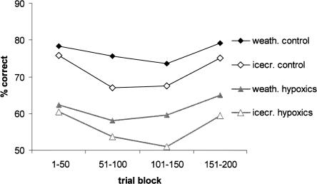
Figure 8 shows the learning curves for both tasks. Performance of 15 hypoxic participants was lower than that of 15 controls (F_1,26 = 21.87, P < 0.001). The precise task (Weather vs. Ice Cream cover story) had no effect on performance (F < 1), nor was there an interaction between task and group (F < 1). The task also did not affect the trial of first strategy use (F_1,19 = 2.29, P > 0.1), the number of strategy switches (F < 1), or the last strategy used [χ²(3) = 1.05, P > 0.5]. We will therefore disregard this variable, and pool data from the two tasks.

Figure 8.

Learning curve for amnesic and control participants in the study of Hopkins et al. (2004), for both the Weather task and the Ice Cream task, which has the same structure but a different cover story.

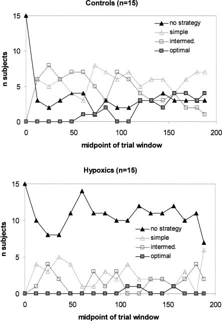
Figure 9 shows strategy use for hypoxic and control participants. Early in training, some participants in each group adopt simple strategies, while others do not. To investigate whether controls and patients used the same strategies, we performed χ² tests for each window with group (2 levels) and strategy cluster as factors. Strategy cluster refers to the grouping of strategies given in Table 1, and has five levels. No difference between the groups was apparent in the first window [from trials 1–24, χ²(3) = 7.74, P > 0.05], the second window [trials 13–36, χ²(3) = 1.67, P > 0.5], or the third window [trials 25–48, χ²(3) = 4.36, P > 0.2]. There was also no group difference in when the first strategy was adopted (F_1,19 = 12.89, P > 0.1) (Table 3). The analysis has as caveats that identification of the trial of first strategy use is impossible if it occurs within the first window, and that six hypoxic participants and one control did not develop any strategy and were excluded from the analysis.

Figure 9.

Best-fitting strategy over windows of 24 trials, for (A) control participants and (B) hypoxic participants in Experiment 3. Strategies are grouped as in Figure 6.

Later in the experiment, performance of the two groups diverged. Across all 200 trials, the control participants switched strategy more often than did the hypoxic patients (F_1,26 = 6.57, P = 0.016) (Table 3). Almost all of these switches were switches from one category cluster to a different one (88% of switches in controls, 96% of switches in patients). Moreover, the groups differed in terms of which strategies were adopted later in the experiment. Strategy use diverged by the fourth trial window [trials 37–60, χ²(3) = 10.27, P = 0.016], and remained different for the two groups in later windows [χ²(3) ≥ 8.77, P ≤ 0.033], with the exception of the 12th window, in which there was only a trend toward a difference (P > 0.05). To investigate how strategy use evolved over time, we regressed the number of persons using a strategy cluster to trial window. Over time, more controls used the optimal strategy (b = 0.277, F_1,15 = 43.38, P < 0.001), while fewer used intermediate strategies (b = −0.228, F_1,15 = 4.63, P = 0.048). There was no change in the number of normal controls using either a simple or no strategy, and none of the strategy clusters were significantly changed over the course of the experiment for patients. While controls thus tended toward the optimal strategy, hypoxics were as likely to be fit by no strategy at all as by another strategy after a strategy switch. Patients were thus learning the task more slowly than controls, and were not adopting more complex strategies at the rate that controls did.

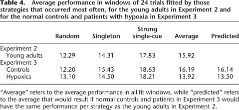
In a separate analysis, we investigated whether the difference in strategy use might explain the lower performance of patients. For every strategy, we computed the average number of correct responses within windows best fit by the strategy. We then compared performance of controls and patients in the current experiment with that of the young adults who participated in Experiment 2. For no strategy was there a difference in performance between groups. (See Table 4 for three strategies that were common in all three groups.) We also investigated whether strategy use could explain the performance of controls and patients in Experiment 3. For each participant, we computed what performance would have been if he or she had had, for each strategy used, as many trials correct as young adults using the same strategy. The performance predicted in this way was close to the actual score for both groups (Table 4). We performed the same analysis in a slightly different way by regressing the number of errors in the trial windows of all participants in Experiment 3 to three factors: First, the group of the participant (control or patient); second, the order of the window in the experiment; and third, the average errors of the strategy fitted to the window. This latter factor explained most of the variance, with a b coefficient of 0.951 [t₍₂₇₀₎ = 16.2, P < 0.001]. Window order had a small effect, with later windows having slightly fewer errors in them than earlier windows, independent of strategy [b coefficient = 0.072, t₍₂₇₀₎ = 2.41, P = 0.017]. Group membership had no effect [t₍₂₇₀₎ = 0.018, P = 0.696]; there was thus no difference between controls and patients in the number of errors made once the strategies used were taken into account. This suggests that differing strategy use can explain the lower number of trials correct of patients relative to controls.

Table 4.

Average performance in windows of 24 trials fitted by those strategies that occurred most often, for the young adults in Experiment 2 and for the normal controls and patients with hypoxia in Experiment 3

“Average” refers to the average performance in all fit windows, while “predicted” refers to the average that would result if normal controls and patients in Experiment 3 would have the same performance per strategy as the young adults in Experiment 2.

Previous results have shown that amnesic individuals are impaired on the Weather task relative to controls, with this difference emerging most clearly late in training (Knowlton et al. 1994; Hopkins et al. 2004). Our current results give a novel explanation for this finding. At the start of learning, there is little that differentiates between how hypoxic patients and control participants perform in the task. In both groups, some participants adopt simple strategies, and others do not. Differences do appear quite early in learning (i.e., around trial 40). Normal controls appear better able to integrate information over the course of learning, and gradually move to more complex strategies. Hypoxic patients, on the other hand, fall back to having no strategy as often as they move to a different strategy. This suggests that the patients are unable to keep track of attempted strategies, and of feedback received over the course of the experiment. Such an inability to keep track would fit with the general pattern of abnormally rapid forgetting in amnesic patients.

Discussion

In our introduction, we posed three questions: (1) Can strategy analysis in probabilistic categorization work in principle? (2) Does it work in practice? (3) Can it offer a new perspective on probabilistic categorization? To answer the first question, we presented Monte Carlo simulations (Experiment 1) that showed that both strategies and strategy switches can be identified in simulated data. To answer the other two questions, we applied the analyses to existing data sets from human categorizers. In Experiment 2, we analyzed categorization performance of normal undergraduates. Our analyses showed that learning is far less linear than is evident from traditional learning curves. Most categorizers switch strategy several times during the course of the experiment, and not all these switches are advantageous: Categorizers sometimes abandon good strategies for less advantageous ones. Experiment 2 also showed that the fitted strategy is a good predictor of responses, which validates our approach. In Experiment 3, we applied our analysis to patients with amnesia. Patients and controls adopted their first strategy at approximately the same point in the experiment, but whereas controls went on to adopt better strategies, patients with amnesia switched strategy less often and, when they did switch, were as likely to adopt a worse as a better strategy.

The analyses as presented here are an extension of those presented by Gluck et al. (2002) and used by Hopkins et al. (2004). The basic results—that the hypoxic group was more likely to use ineffective strategies than the control group—are the same here as previously reported by Hopkins et al. (2004). But the new analysis provides several additional benefits, of which the most evident is the ability to search for switch points, trials on which participants switch from one strategy to another. This allowed us to identify another group difference: Although the hypoxic group was as quick to adopt an initial strategy as the control group, they were less able to switch to a better strategy—both because they switched fewer times in general and also because their switches were more likely to lead to a “worse” strategy that resulted in fewer correct responses.

Another improvement of the new analysis is the ability to consider a random strategy. Participants who did not have a clear strategy or did not consistently follow one were best fit by this “strategy.” In the method of Gluck et al. (2002), these participants would be best fit by a singleton strategy (one in which only patterns with one cue would be responded to correctly). Thus, participants who were responding randomly (or according to some other unknown strategy) would be incorrectly classed. Using the new analysis, participants are only classed as responding based on the singleton strategy if that strategy fits their data better than a random strategy. As a result, whereas Gluck et al. (2002) reported that nearly 87% of their healthy young adults were best fit by a simple (singleton or single-cue) strategy, Figure 6 shows a drastic reduction in that proportion. Conversely, when (as shown in Fig. 9B) the hypoxic group is found to be best fit by a random strategy in the new analysis, this is a much more powerful statement than was possible via the previous analysis.

A third difference from the earlier analysis method is that the metric for fitting strategies has been changed from squared error minimization to a maximum likelihood approach.¹¹

How do people solve the Weather task?

We here proposed a way of analyzing probabilistic categorization, not a new theory on how participants actually perform probabilistic categorization tasks. We do not propose that different strategies reflect different modes, or that different brain systems are responsible for responses generated with different strategies. Nevertheless, the analysis has several assumptions that make it more compatible with some hypotheses about probabilistic categorization, and less with others.

There are many possible ways in which people could solve probabilistic categorization tasks. One possibility is that categorizers use one consistent rule to categorize all stimuli (e.g., if the square card is present, then respond “sun,” or else respond “rain”). This could be either a conscious, verbalizable rule, or one that is implicit (not directly amenable to conscious recall). If categorizers do not have one rule, they could base responses mostly on individual patterns (e.g., the pattern with one square card and one circle card means “sun”; or the pattern with one square card and one diamond card means “rain”) or on individual cards (e.g., the square card means “sun” with 80% reliability, while the circle card means “sun” with a mere 60% reliability). Again, these associations could be learned consciously through memorization, or implicitly through gradual learning of stimulus–response outcomes. And to the extent that a healthy human brain is capable of multiple forms of learning, an individual may engage in multiple kinds of learning simultaneously.

These are not the only ways imaginable, but certainly ones that have been proposed in the literature. The idea of a verbalizable rule would follow if participants engage in explicit hypothesis testing during probabilistic categorization. Exemplar theories (e.g., Nosofsky and Palmeri 1997), on the other hand, are most consistent with gradual learning of associations between patterns and outcomes, while a conditioning approach (Gluck and Bower 1988; Gluck, 1991) is consistent with the gradual acquisition of either pattern–outcome associations or cue–outcome associations (depending on what one takes as the input of the conditioning process.)

Currently, all options are still viable. Most debated has been the possibility of hypothesis testing. This is what participants tend to engage in during deterministic classification with few cues (e.g., Raijmakers et al. 2001), suggesting that participants in probabilistic categorization might start out with hypothesis testing as the default strategy. Gluck et al. (2002) found that most participants in a probabilistic categorization task were unable to verbally state a rule they were following. Even in those who did volunteer one, the verbal rule did not reliably predict actual behavior. However, their participants reported retrospectively on their behavior, and it is well known that participants during task performance may be aware of more than they will report after the task is completed (Ericsson and Simon 1984).

Our strategy analysis makes two assumptions, namely, that there are stable states in performance that map onto the strategies our analysis searches for, and that learning involves rather discrete switches that typically involve all patterns at once. The first assumption could be reconciled with all options. The second assumption only fits with the options in which categorizers use a consistent rule in their categorization. If responses to each pattern evolve independently of one another, as suggested by options in which responses are based on pattern–outcome or cue–outcome associations, then switches will typically not affect all patterns at once; thus they will not be equivalent to the kind of switches our analysis looks for.

Whether our two assumptions are true is ultimately an empirical question. The only way to answer it is to compare the ability of our analysis to predict responses with that of well-formulated alternatives. The fact that our analysis was a better predictor of responses than either previous responses or previous outcomes suggests that simple pattern-based learning approaches will not be very promising.

Conclusions

Here, we have shown that the analysis can work, and can bring new insights in probabilistic categorization. The analyses can reliably identify strategies if they are used, and can identify switches from one strategy to another. Moreover, the fitted strategy can predict responses. The analyses show learning to be highly nonlinear in probabilistic categorization, and suggest that patients with hippocampal damage can change strategies but are as likely to fall back to an inferior strategy as to move to more beneficial ones.

Materials and Methods

Details of fitting procedure

Strategy analysis was done by computing the likelihood of a given set of responses by the participant given that that participant was following a certain strategy. These strategies were predefined, and consisted of those that yielded better performance than random responding and that can be succinctly described. Those that cannot be succinctly described were assumed to be too difficult to use. Table 1 gives the likelihood of responding “sun” to each pattern for a strategy, and can be used to generate the likelihood of a set of responses given that the strategy is used. In particular, the likelihood of, in a given window, responding x times “sun” to pattern A and y times “rain” is given by the binomial distribution. The likelihood of all responses in a window is the likelihood of the responses given to each pattern multiplied with one another.

A strategy was ascribed to the participant if it generated the highest likelihood of the data, and if this likelihood was meaningfully higher than that generated by “random” behavior (a 50–50 likelihood of each answer independent of the presented pattern). This was defined as having a lower AIC, with one parameter distinguishing between fitting the best strategy and fitting only the “random” strategy. This was done because the analysis can be reformulated into a model in which one parameter, s, defines which strategy fits best. The likelihood of answering “sun” to pattern i, π_i,_s, then is:

where δ(j − s) is the Dirac function that is 1 if j = s and 0 otherwise, and π_i,s the likelihood of answering “sun” to pattern i given strategy s, as given in Table 1.

We fit strategies to both the last 40 trials of a session, and across the sequence of responses generated by a participant. We also fit them to moving windows of 24 trials. One such window of trials was fit each 12 trials (i.e., adjacent windows overlapped in 50% of their trials). If at least two subsequent windows were best fit by the same strategy, we labeled these as a consistent block of strategy use. The reported numbers of strategies used are equal to the number of such consistent blocks. One extra strategy switch was counted for an initial adoption of a strategy other than “random” behavior.

If participants are first consistently following one strategy and then later another, a strategy switch in between can be assumed. In between each two blocks of consistent strategy use, we searched for strategy switches by identifying the points, which we refer to as extreme points, at which (1) the change in fit of the previous strategy was maximal, (2) the change in fit of the following strategy was maximal, and (3) all strategies together exhibited the maximum change in fit. If two of these three extreme points occurred within four trials of each other, their midpoint was taken as the moment of strategy switch. If no two extreme points occurred in each other’s proximity, the interval between the extreme points was labeled as an “area of insecurity.” The extreme points are the extreme points of the derivative of the fitting functions (i.e., the inflection points). As these derivatives cannot be computed, we estimated them by subtracting the fit of the 12 trials before an analyzed trial from the 12 trials after the analyzed trial. (We also experimented with using more than 12 trials in these analyses—this did not substantially change the number of switches identified or correctly localized.) Extreme points were those at which this difference function peaked or had a minimum.

A special case is the first strategy to appear. In some participants, the first windows of trials were best fit by the “random” strategy (assuming nothing more than gambling), and a switch to another strategy could be established in later windows through the analysis discussed above. If a strategy other than the “random” one fitted on the first window, the analysis could not be run. In such cases, we set the trial at which the first strategy appeared to six. Our rationale for this choice was that for the strategy to fit on the first window, it must have been adopted somewhere between trial 1 and trial 12.

Experiment 2

We analyzed data first reported by Gluck et al. (2002), Experiment 2. In brief, participants were 30 Rutgers University undergraduates (17 females, 13 males, mean age 20.7 yr), who received credit in an introductory psychology class for their participation. They were given a 200-trial Weather Prediction task, in which they were given one of 14 patterns consisting of the cards shown in Figure 1, and given a choice of either rain or sun. Two hundred trials were generated to satisfy the card-outcome probabilities shown in that figure; ordering of these trials was randomized but fixed across subjects. After their response, participants received visual feedback about the actual Weather outcome. Responses were scored as “optimal” based on whether participants predicted the Weather outcome most often associated with the current pattern, independent of whether the participants predicted the actual weather on any given trial.

Experiment 3

Participants in the Weather task were seven patients who became densely amnesic after a hypoxic injury (four females, three males, mean age 41.1 yr). Bilateral hippocampal damage was confirmed by radiology (MRI or CT) in five of the seven patients. Seven healthy adults, matched for age and education to the patient group, served as controls. Participants were given the Weather task described earlier in Experiment 2. Eight patients (five females, three males, mean age 39.8 yr) participated in the Ice Cream task, six of which had also done the Weather task. Controls were eight healthy adults, matched for age and education to the patient group. The Ice Cream task is structurally identical to the Weather task, but has a different cover story. Instead of having to guess the weather from Tarot cards, participants had to guess what flavor a photographed figure (Mr. Potatohead) would like. The figure could vary on four dimensions: whether or not he had a moustache, a hat, eyeglasses, and a bow tie. These four played the role of the four cards in the Weather task. For full details of patients and procedure, see Hopkins et al. (2004).

References

- Aron A.R., Shohamy D., Clark J., Myers C.E., Gluck M.A., Poldrack R.A. Human midbrain sensitivity to cognitive feedback and uncertainty during classification learning. J. Neurophysiol. 2004;92:1144–1152. doi: 10.1152/jn.01209.2003. [DOI] [PubMed] [Google Scholar]
- Ashby F.G., Alfonso-Reese L.A., Turken A.U., Waldron E.M. A neuropsychological theory of multiple systems in category learning. Psychol. Rev. 1998;105:442–481. doi: 10.1037/0033-295x.105.3.442. [DOI] [PubMed] [Google Scholar]
- Ericsson K.A., Simon H.A.1984. Protocol analysis: Verbal reports as data. MIT Press; Cambridge, MA. [Google Scholar]
- Estes W.K. Learning theory and the new “mental chemistry.”. Psychol. Rev. 1960;67:207–223. doi: 10.1037/h0041624. [DOI] [PubMed] [Google Scholar]
- Gallistel C.R., Fairhurst S., Balsam P. The learning curve: Implications of a quantitative analysis. Proc. Natl. Acad. Sci. 2004;101:13124–13131. doi: 10.1073/pnas.0404965101. [DOI] [PMC free article] [PubMed] [Google Scholar]
- Gluck M.A. Stimulus generalization and representation in adaptive network models of category learning. Psychol. Sci. 1991;2:1–6. [Google Scholar]
- Gluck M.A., Bower G.H. From conditioning to category learning: An adaptive network model. J. Exp. Psychol. Gen. 1988;117:225–244. doi: 10.1037//0096-3445.117.3.227. [DOI] [PubMed] [Google Scholar]
- Gluck M.A., Shohamy D., Myers C.E. How do people solve the “weather prediction” task? Individual variability in strategies for probabilistic category learning. Learn. Mem. 2002;9:408–418. doi: 10.1101/lm.45202. [DOI] [PMC free article] [PubMed] [Google Scholar]
- Hopkins R.O., Myers C.E., Shohamy D., Grossman S., Gluck M.A. Impaired probabilistic category learning in hypoxic subjects with hippocampal damage. Neuropsychologia. 2004;42:524–535. doi: 10.1016/j.neuropsychologia.2003.09.005. [DOI] [PubMed] [Google Scholar]
- Knowlton B.J., Squire L.R., Gluck M.A. Probabilistic classification learning in amnesia. Learn. Mem. 1994;1:1–15. [PubMed] [Google Scholar]
- Knowlton B.J., Squire L., Paulsen J., Swerdlow N., Swenson M., Butters N. Dissociations within nondeclarative memory in Huntington’s disease. Neuropsychology. 1996;10:538–548. [Google Scholar]
- Nosofsky R.M., Palmeri T.J. An exemplar-based random walk model of speeded classification. Psychol. Rev. 1997;104:266–300. doi: 10.1037/0033-295x.104.2.266. [DOI] [PubMed] [Google Scholar]
- Poldrack R.A., Clark J., Pare-Blagoev E.J., Shohamy D., Creso Moyano J., Myers C.E., Gluck M.A. Interactive memory systems in the human brain. Nature. 2001;414:546–550. doi: 10.1038/35107080. [DOI] [PubMed] [Google Scholar]
- Raijmakers M.E.J., Dolan C.V., Molenaar P.C.M. Finite mixture distribution models of simple discrimination learning. Mem. Cognit. 2001;29:659–677. doi: 10.3758/bf03200469. [DOI] [PubMed] [Google Scholar]
- Restle F. Significance of all-or-none learning. Psychol. Bull. 1965;64:313–325. doi: 10.1037/h0022536. [DOI] [PubMed] [Google Scholar]
- Rodriguez P., Aron A.R., Poldrack R.A.2006. Ventral striatal/nucleus-accumbens sensitivity to prediction errors during classification learning. Human Brain Mapping. (in press). [DOI] [PMC free article] [PubMed] [Google Scholar]
- Shohamy D., Myers C.E., Onlaor S., Gluck M.A. Role of the basal ganglia in category learning: How do patients with Parkinson’s disease learn? Behav. Neurosci. 2004;118:676–686. doi: 10.1037/0735-7044.118.4.676. [DOI] [PubMed] [Google Scholar]