Weighting of experimental evidence in macromolecular structure determination

Abstract

The determination of macromolecular structures requires weighting of experimental evidence relative to prior physical information. Although it can critically affect the quality of the calculated structures, experimental data are routinely weighted on an empirical basis. At present, cross-validation is the most rigorous method to determine the best weight. We describe a general method to adaptively weight experimental data in the course of structure calculation. It is further shown that the necessity to define weights for the data can be completely alleviated. We demonstrate the method on a structure calculation from NMR data and find that the resulting structures are optimal in terms of accuracy and structural quality. Our method is devoid of the bias imposed by an empirical choice of the weight and has some advantages over estimating the weight by cross-validation.

Experimental data are typically insufficient to determine a biomolecular structure in their own right but need to be complemented with prior physical information. Therefore, structure determination amounts to the search for conformations that have a low physical energy and that, at the same time, minimize a cost function E_data quantifying the disagreement between a structural model X and the data. This approach is implemented as minimization of a hybrid energy (1, 2)

where the force field E_phys compensates a lack of data by imposing physical constraints on the structure. A target function of this form is widely used in macromolecular structure determination, notably from NMR data (3, 4) and from homology-derived restraints (5). The weight w_data controls the contribution of the data relative to the force field. Its value can be critical: If it is too large, the contribution of the force field might be too small to avoid overfitting; if the weight is too small, the data contribute too little to define the structure. The choice of the weight also concerns the question of how to judge structural quality. Overfitted structures reach a low R value (6, 7) but exhibit a poor stereochemistry or an unlikely fold.

Usually, experimental data are weighted empirically: w_data is set ad hoc and held constant during structure calculation. However, already when introducing the hybrid energy concept, Jack and Levitt (1) remarked that correct weighting of the data “is something of a problem.” They proposed to adjust the weight to equalize E_phys and w_dataE_data; this adjustment was later refined, for example, in ref. 8. At present, the most rigorous quantitative method to determine the optimal weight is complete cross-validation (6, 7). However, cross-validation can become unstable and time-consuming in the case of sparse and heterogeneous data with several independent weights.

In this work, we introduce an objective and unique way to weight experimental data. We show that a quantitative treatment does not necessitate heuristics like cross-validation: everything we need is contained in the rules of probability theory.

Theory

Inferential Structure Determination.

We recently introduced a probabilistic approach to structure determination (9, 10), which permits the estimation of unknowns, such as theory parameters, in addition to the conformational degrees of freedom. We represent the unknown structure through a conditional probability p(X) = dP(X|D, I)/dX that quantifies the likelihood of X being the true molecular structure in light of the data D and of relevant prior knowledge I. The posterior distribution p(X) spreads the uncertainty about the structure over the entire conformational space and peaks in regions where conformations are in accord with the data and the prior knowledge. Bayes’ theorem (11) states that the posterior distribution is proportional to the product of the likelihood function L(X) and the prior distribution π(X): p(X) ∝ L(X)π(X). The likelihood function derives from the probability of observing the measurements given the molecular structure, i.e., L(X) = P(D|X, I). The conformational prior distribution π(X) = dP(X|I)/dX represents general knowledge about the unknown structure of the target molecule. If the mean energy or likewise the temperature β⁻¹ of the system is known, the Boltzmann distribution π(X) ∝ exp{−βE_phys(X)} is the least biasing prior distribution (12). The most probable conformations minimize the negative logarithm of the posterior distribution, and we can establish a formal analogy to hybrid energy minimization: −logπ corresponds to the force field E_phys because it describes a priori meaningful structures; −logL is similar to w_dataE_data because it penalizes structures that do not fit the data.

We model the data as independent measurements and use a distance measure δ(y_i, y_i(X)) to evaluate the discrepancy between the ith observation y_i and its prediction y_i(X). Thus, the likelihood of the data is

This likelihood function is of the least-squares type with χ²(X) = Σ_i[δ(y_i, y_i(X))]² evaluating the average disagreement between backcalculated and observed data. The residual χ² is minimal if the theory exactly matches the experiment; the factor Z(σ) normalizes the likelihood function with respect to the data (i.e., Z(σ) = ∏_i∫dy_ie^−(1/2σ2)[δ(y_i, y_i(X))]²). In case of Gaussian data, for example, we have δ(y_i, y_i(X)) = y_i − y_i(X) and obtain Z(σ) = (2πσ²)^n/2, χ²(X) = Σ_i=1ⁿ [y_i − y_i(X)]²; σ is the standard deviation of the measurements.

Joint Posterior Distribution.

In general, the parameter σ evaluates to which extent the structure can be fit to the data and serves as a “unit” of the distance measure δ. It depends on both the quality of the data and the precision of the theory used to backcalculate the data. Therefore, σ can be viewed as an “error” that includes experimental noise as well as systematic contributions. In practice, this error is unknown, just like the coordinates. When evaluating the likelihood function for a conformation, we have to set σ and are facing the same dilemma as in the hybrid energy approach where w_data is unknown. Consequently, we need to consider the likelihood factor not only a function of the coordinates but also of the error. We symbolize this dependence explicitly through L_joint(X, σ) instead of L(X).

The essence of Bayesian inference is that probabilities can be attributed to any statement, not only to those concerning “random variables.” Probabilities express ignorance. If both X and σ are unknown, the bearing of the data on them is quantified by a joint posterior distribution p_joint(X, σ); p_joint is a probability distribution for the unknown coordinates and the unknown error. Formally, this distribution is obtained by replacing X with (X, σ) in Bayes’ theorem. To this end, we introduce a joint prior distribution π(X, σ) = π(σ|X)π(X). Because knowledge of the coordinates has no bearing on the error, we obtain

as joint posterior distribution for all unknowns, i.e., for X and σ. Usually, concrete prior knowledge about the error is lacking. However, we know that σ is positive and that its value has no absolute meaning, because it depends on the units of the distance measure δ. Changes in the units of δ can be compensated by scaling the error appropriately. Therefore, π(σ) should be invariant under scaling, leading to π(σ) = σ⁻¹ (13).

The joint posterior distribution p_joint summarizes our knowledge about the structure and the error, and all inferences on these unknowns can be derived from p_joint. Usually, one is primarily interested in the coordinates and not in the error. The statistically correct way to eliminate the error is to integrate over all possible values of σ. This so-called marginalization (11) projects the joint posterior distribution to conformational space: The marginal posterior distribution p_marginal(X) = ∫dσp_joint(X, σ) no longer involves an error parameter. We can either use p_marginal(X) or the integrated likelihood function (14) L_marginal(X) = ∫dσL_joint(X, σ)π(σ) to determine the structure. Often, marginalization integrals can be solved analytically. Complicated models, however, require the use of numerical integration techniques. Analytical calculation of L_marginal(X) avoids the problem of choosing an appropriate weight from the start. The error is then only introduced to devise the likelihood function and eliminated afterward by marginalization.

Results

To demonstrate the outlined formalism, we analyzed NMR-derived distance measurements for the protein ubiquitin (15) (Protein Data Bank ID code 1d3z). We extracted from the deposited 2, 727 interproton distances 1, 444 nonredundant entries by retaining only the smallest distance in case multiple measurements were available for the same pair of protons. Because distances are nonnegative, we model deviations between n measured and calculated distances with a lognormal distribution (16):

for this choice χ²(X) = Σ_ilog²[d_i/d_i(X)] and Z(σ) = (2πσ²)^n/2. We used posterior simulation techniques (17) to calculate structures and to simultaneously estimate the error of the lognormal model. Structures were parameterized in torsion angles; nonbonded interactions were represented with a purely repulsive potential (18). Simulations of the posterior distributions were carried out with our software for inferential structure determination (isd; M.H. and W.R., unpublished results) using the random sampling strategies outlined in refs. 9, 10, and 19.

Impact of the Weight on Structural Quality.

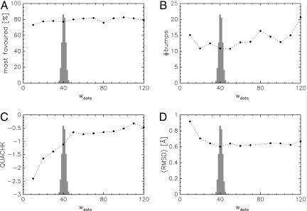
We first calculated structures for fixed weights by simulating the conditional conformational posterior distribution p_joint(X, σ = 1/$\sqrt{w_{\mathrm{data}}}$) ∝ exp{−w_dataχ²(X)/2 − βE_phys(X)}. These simulations correspond to hybrid energy minimizations with a constant weight. We used the hybrid Monte Carlo method (20) embedded in a Replica-exchange Monte Carlo scheme (19) to generate conformational samples. Fig. 1 shows the average values for several validation criteria calculated for the 50 most likely conformations. The Ramachandran statistics are almost independent of the weight. The number of bumps tends to increase with the weight, because structures become more compact, if the data contribute more. The what if (22) quality index increases with the weight, an almost constant value is reached for w_data ≥ 50. An optimal weight w_data ≈ 40 exists for which the structures will be most accurate, as measured by the root mean square difference (rmsd) to the x-ray structure (23) for the atoms N, C^α, C of the protein backbone.

Fig. 1.

Influence of weight on different aspects of structural quality. (A) Ramachandran statistics [calculated with procheck (21)]. (B) Number of bumps as calculated with what if (22). (C) what if quality index QUACHK. (D) Average rmsd to the crystal structure (23). The shaded histogram p(w_data) results from a Bayesian calculation.

Probabilistic Interpretation.

Because the logarithm is a monotonically increasing function, maximization of the posterior probability can be achieved by minimizing its logarithm. Therefore, the negative logarithm of the joint posterior distribution, −logp_joint(X, σ) = −log[L_joint(X, σ)π(X)π(σ)], can be interpreted as a joint hybrid energy E_joint(X, σ) now depending not only on the coordinates but also on the error. If we insert L_joint and our choices for the prior distributions π(X) (Boltzmann factor) and π(σ) and neglect constants that neither depend on the structure nor on the error, we obtain

as an extended joint hybrid energy. The equivalences E_data(X) = χ²(X)/2 and w_data = 1/σ² clarify the nature of the weight: It is not merely a fudge factor but quantifies the quality of the data and the reliability of the theoretical model used to predict them. If observed and backcalculated data are in good agreement, σ will be small and w_data large. In case of disagreement, σ will be big and w_data small. By choosing the error appropriately, we balance the contribution of experimental and prior information. The joint hybrid energy (Eq. 5) E_joint(X, σ) = E_hybrid(X) + log[Z(σ)/π(σ)] contains a term, log[Z(σ)/π(σ)], not included in the standard target function E_hybrid (Eq. 1). Only this additional term allows us to determine the error. To derive this “regularizer” for σ, the use of a probabilistic framework for structure determination is indispensible: Z(σ) originates in the normalization of P(D|X, I), π(σ) is required by Bayes’ theorem: both terms are missing in purely optimization-based approaches where normalization constants and prior probabilities are usually not incorporated.

Estimation of the Weight.

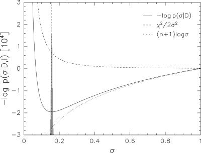
For Model 4, it holds that Z(σ)/π(σ) ∝ σⁿ⁺¹. In the joint target function E_joint (Eq. 5), two contributions counterbalance each other: χ²/σ² decreases when σ increases, thus preferring large values for the error when E_hybrid is minimized with respect to the error. The additional term log[Z(σ)/π(σ)] = (n + 1)logσ is monotonically increasing and favors small errors (see Fig. 2). Thus, only when log[Z(σ)/π(σ)] is added to the standard hybrid energy, one obtains a joint hybrid energy that exhibits a finite minimum in σ and can directly be used to determine the error or, likewise, the weight from the data. Minimization of the resulting joint hybrid energy E_joint(X, σ) yields the most probable structure X_max and the most probable error σ_max. In case of model 4, we have σ_max = $\sqrt{\chi (X_{\max })/(n}+1)\text{.}$

Fig. 2.

Contributions in the joint hybrid energy E_joint(X, σ) that determine the error. The black solid curve indicates the overall dependence on the error. The dashed line shows the dependence on the term χ²/2σ², which appears in the standard hybrid energy; the dotted line is the contribution from the regularizer log[Z(σ)/π(σ)]. The shaded histogram is the result of a Bayesian analysis (also shown in Fig. 1 for w_data = 1/σ²) and is peaked about the optimal value (vertical dotted line).

In our approach, we do not minimize E_joint(X, σ) but rather draw random samples from the joint posterior distribution p_joint(X, σ) using a Gibbs sampling scheme (24). In this scheme, samples of the coordinates and the error are drawn in an iterative fashion by alternately setting σ or X to the previous sample in the joint posterior distribution. When the error is fixed in p_joint(X, σ), we again obtain a distribution that is proportional to exp{−E_hybrid(X)} and that can be sampled using the hybrid Monte Carlo method. If we fix the coordinates to the most recent conformational sample, we obtain a probability distribution for the error that is proportional to σ⁻⁽ⁿ⁺¹⁾exp{−χ²(X)/2σ²}. By substituting σ with 1/$\sqrt{w_{\mathrm{data}}}$ we notice that for fixed conformational degrees of freedom the weight follows a gamma distribution (10)

.

We thus can sample the weight or, likewise, the error using a random number generator for the gamma distribution. The resulting histogram is shown in Fig. 1 and demonstrates that the coordinates and the weight can be estimated simultaneously. The optimal weights sampled by our algorithm lie within the region where the what if quality scores reach their best values. Moreover, the weights scatter around a most likely value (≈40) leading to conformations that are closest to the x-ray structure when the weight is fixed during structure calculation. Thus, our algorithm adapts the weight to yield optimal structures in terms of accuracy (rmsd to the x-ray structure).

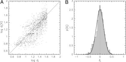
How is it possible to estimate the coordinates and the error simultaneously? Intuitively, the true molecular structure minimizes the deviations between observed and calculated data. If we knew the correct structure, the weight would just reflect the width of the distribution of deviations between observations and predictions. Assuming no systematic errors, the distribution of the discrepancies δ_i = log[d_i/d_i(X)] will ideally be a zero-centered Gaussian with standard deviation $\hat{\sigma }$ = $\sqrt{(1/n){\sum }_i{\delta }_i^2\text{.}}$ Fig. 3 shows that this is indeed the case for the analyzed data set using the log-ratio as distance measure and considering the NMR structure 1d3z (15) the “true” structure.

Fig. 3.

Comparison between experimental distances and distances found in the structure 1d3z. (A) Scatter plot of the logarithm of the distances d_i(X) in 1d3z vs. the logarithms of the experimental distances d_i. (B) The shaded histogram indicates the distribution of deviations δ_i = log[d_i/d_i(X)] between the measured and predicted distances. The black solid line is a zero-centered Gaussian with width 1/ $\sqrt{w_{\mathrm{data}}}$, where w_data was set to the optimal value 40.

This intuitive behavior of the weight is contained in our formulation. As outlined before, the posterior distribution of the weight given the structure is a gamma distribution (cf. Eq. 6). Thus, we obtain 〈w_data〉 = n/χ²(X) as an estimate for the unknown weight; this estimate is identical to the intuitive estimate 1/$\hat{\sigma }$². Because we are working with probabilities, we can further assess the estimate’s precision by its standard deviation $\sqrt{2n}$ ∕χ² = $\sqrt{2∕n}$ 〈w_data〉. The residual χ² is approximately extensive, meaning that it increases if we add more data. That is, our approach concurs with common sense: the average weight quantifies, in good approximation, how well the structure fits the data, independent of the size of the data set. In contrast, the precision of the estimate, measured by the width of the weight distribution, decreases rapidly as the number of data grows, because Δw_data ∝ 1∕ $\sqrt{n\text{.}}$ For typical NMR data, we thus obtain sharp distributions, but even for sparse data these distributions remain well defined (cf. ref. 9).

Elimination of the Weight.

As mentioned in Theory, it is sometimes possible to integrate out the error in the likelihood function. For Model 4, this calculation is straightforward: The marginal likelihood is proportional to ∫dσσ⁻⁽ⁿ⁺¹⁾exp{−χ²(X)/2σ²}; like in the derivation of Eq. 6 we can substitute σ with 1∕$\sqrt{w_{\mathrm{data}}}$ and observe that the required integral is just the normalization constant of the gamma distribution. Therefore, L_marginal(X) ∝ [χ²(X)]^−n/2 where the suppressed proportionality constant does not depend on the coordinates. L_marginal(X) cannot be written as a product of probabilities that involve only a single measurement; it is a composite probability for the whole data set. By taking the negative logarithm of the marginal posterior distribution p_marginal(X) ∝ L_marginal(X)π(X), we devise a target function for the coordinates only

.

Because the weight is not completely determined by the data but adopts different values for different structures, the marginal hybrid energy is less pronounced than the standard hybrid energy: The least-squares residual is transformed logarithmically and weighted with the number of measurements. The marginal hybrid energy (Eq. 7) is less biased than the hybrid energy (Eq. 1) because it relies on the data only and does not assume knowledge of the weight.

There exists a close relation to the joint hybrid energy (Eq. 5). We can turn the argument that led to our estimate 〈w_data〉 around by stating that every conformation X requires its own weight n/χ²(X). Therefore, one can eliminate the weight heuristically by considering E_joint(X, σ = $\sqrt{{\chi }^2(X)∕n}$ ) a target function that only involves the coordinates. The resulting target function, (n + 1)/2 logχ²(X) + βE_phys(X), is almost identical to Eq. 7.

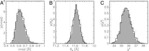
Regarding the conformational degrees of freedom, the marginal posterior distribution p_marginal(X) and the joint posterior distribution p_joint(X, σ) contain the same information: Sampling p_joint(X, σ) can be viewed as numerically integrating out the error. A simulation of p_marginal(X) confirms the equivalence of the joint and the marginal posterior distribution also in practice (Fig. 4). For both simulations, we obtain a rmsd of 0.63 ± 0.06 Å to the crystal structure (the optimal value w_data = 40 resulted in a rmsd of 0.60 ± 0.05 Å). The similarity of the distribution of rmsd, radius of gyration, and χ² indicates the equivalence of both simulations.

Fig. 4.

Equivalence of the simulations of joint and marginal posterior distribution. The solid curves are the posterior histograms from a simulation of the marginal posterior distribution p_marginal(X); the shaded histograms are the results for p_joint(X, σ). (A) Distribution of rmsd values to the crystal structure; the dotted line indicates the average rmsd obtained for w_data = 40 (see also Fig. 1D). (B) Distribution of the radii of gyration; the dotted line indicates the radius of gyration of the x-ray structure. (C) Distribution of the least-squares residual χ².

Comparison with Cross-Validation.

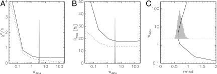
Cross-validation (7) is based on the idea that the weight should be chosen such that overfitting is prevented. The data are divided into two nonoverlapping sets: a working set A that is used for structure calculation and a test set T for which the “free” R value is calculated to assess a certain choice of the weight. Ideally, the optimal weight minimizes the free R value. We randomly divided the 1, 444 distances into 10 sets of approximately equal size and carried out a complete 10-fold cross-validation. We used a simulated annealing protocol (25) implemented in cns (26) to calculate structures for each working set. Because the cost function resulting from the lognormal distribution (4) is not implemented in cns, we used a Gaussian error distribution leading to harmonic terms. For comparison, we simulated the joint posterior distribution for a Gaussian likelihood, i.e., δ_i = d_i − d_i(X), using the isd software.

The result of a complete cross-validation is shown in Fig. 5. By increasing the weight, one can reduce the residual of the working set to smaller and smaller values. In contrast, the fit of the test set becomes slightly worse if the weight is too large (Fig. 5A). The standard R value, χ_T²/Σ_i∈T d_i², is proportional to the residual χ_T² = Σ_i∈T[d_i − d_i(X)]² of the test set. For NOESY data, Brünger et al. (7) used R_1/6 = Σ_i∈T|d_i⁻¹ − d_i⁻¹(X)|/Σ_i∈T d_i⁻¹. Neither of the two free R value curves (Fig. 5B) exhibits a pronounced minimum. Therefore, the choice of the weight by cross-validation remains ambiguous. In contrast, the Bayesian result is very clear-cut. It avoids overfitting by weighting the data as little as possible while maintaining structures of high quality. Fig. 5C again shows that the Bayesian choice is also optimal in terms of accuracy. The distribution of the rmsd to the crystal structure obtained with the Bayesian calculation concentrates at low values and agrees well with the result obtained with cross-validation. As can be seen from the diagram, accuracy changes only little for different weights. For reasons discussed above, we nevertheless obtain sharp posterior histograms for the weight, which demonstrates the high sensitivity of a Bayesian approach.

Fig. 5.

Comparison of cross-validation and Bayesian weighting. The shaded histogram in A and B is the weight distribution p(w_data) using a Gaussian likelihood function. (A) Normalized average residual 〈χ²〉/n of the working set (dotted line) and the test set (solid line). (B) Standard free R value curve (solid line) and free R_1/6 value curve (dotted line). (C) Histogram of rmsd values to the crystal structure for the conformations generated from a Gaussian likelihood function and a corresponding rmsd curve for the structures generated during the cross-validation calculations.

Further advantages of our approach over cross-validation for the purpose of setting the weight are as follows. First, cross-validation contains unspecified elements that still depend on the choice of the user and are not solely determined by the data. The data need to be partitioned, and the choice of a particular weight has to be assessed by an appropriate R value. Because NMR data are usually preprocessed, several R values have been proposed (27), and there exists no consensus as to which R value performs best. Second, cross-validation will be impractical for sparse data because of the reduced size of the working set, whereas the Bayesian algorithm is still stable. All operations such as analytical marginalization or posterior sampling are also valid for data sets much smaller than the one used in the calculations shown here. For example, in ref. 9 we report on a structure determination with only 10% of the data used here for a protein of similar size. Finally, we expect the Bayesian approach to be significantly more efficient than cross-validation. Currently, our implementation relies on posterior sampling techniques that require more computational resources than standard structure calculation methods. However, our findings directly apply to minimization approaches. Instead of minimizing E_hybrid with w_data fixed by some empirical rule, we propose to minimize E_joint or likewise E_marginal using, for example, simulated annealing. Minimization of E_joint or E_marginal is of the same complexity as a minimization of E_hybrid. Therefore, a single minimization of a probabilistically motivated target function can produce the same information as cross-validation calculations that require a whole set of minimization runs.

Conclusions

By using Bayesian inference, we resolved the issue of weighting experimental data in macromolecular structure determination and demonstrated the method on a structure calculation from NMR data. Probability calculus provides definite rules to determine the unknown data weight: It can either be estimated from the data or eliminated analytically by marginalization. Both strategies are equivalent and also could be implemented in minimization-based computer programs.

Our method is objective in the sense that both the weight and the structures are uniquely determined by the experimental data at hand and some additional, but required, assumptions such as the choice of the force field and of the theory used to backcalculate the data.

The probabilistic model describing the data also provides a clear interpretation of the weight as being related to the average discrepancy between observed and calculated data. Thus, the weight quantifies limitations both of the data and of the theory.

The formalism can be applied to a large class of structure calculation problems that are based on hybrid energy minimization. The data term translates into the likelihood function; its normalization constant is obtained by integrating exp{−w_dataE_data(X)} over the data. It is important to incorporate this term into the hybrid energy. One can then use the joint target function (Eq. 5) to determine the coordinates and the optimal weight simultaneously. For example, the formalism is directly applicable to homology modeling and to structure calculation from restraints obtained from FRET or mutagenesis experiments.

However, the proposed formalism does not necessitate the application of posterior sampling techniques. Instead the negative log-posterior distributions could be used for minimization-based structure calculation. In analogy to the Gibbs sampling procedure, the joint hybrid energy E_joint could be minimized by periodically updating the weight with the estimate χ²/n during a simulated annealing run. Alternatively, one could eliminate the weight analytically and minimize E_marginal.

A further advantage of our method is that multiple data sets can be treated in the same way. The Bayesian result is similar to that of a complete cross-validation but more clear-cut and stable. In addition to an estimate of the weight, we obtain its reliability. The estimated weight can be used to assess the quality of the data and may serve as a figure of merit similar to the free R value.

Abbreviation

rmsd

rms difference

References

- 1.Jack A., Levitt M. Acta Crystallogr. A. 1978;34:931–935. [Google Scholar]
- 2.Brünger A. T., Nilges M. Q. Rev. Biophys. 1993;26:49–125. doi: 10.1017/s0033583500003966. [DOI] [PubMed] [Google Scholar]
- 3.Kaptein R., Zuiderweg E. R., Scheek R. M., Boelens R., van Gunsteren W. F. J. Mol. Biol. 1985;182:179–182. doi: 10.1016/0022-2836(85)90036-1. [DOI] [PubMed] [Google Scholar]
- 4.Clore G. M., Gronenborn A. M. Proc. Natl. Acad. Sci. USA. 1998;95:5891–5898. doi: 10.1073/pnas.95.11.5891. [DOI] [PMC free article] [PubMed] [Google Scholar]
- 5.Ŝali A., Blundell T. J. Mol. Biol. 1993;234:779–815. doi: 10.1006/jmbi.1993.1626. [DOI] [PubMed] [Google Scholar]
- 6.Brünger A. T. Nature. 1992;355:472–474. doi: 10.1038/355472a0. [DOI] [PubMed] [Google Scholar]
- 7.Brünger A. T., Clore G. M., Gronenborn A. M., Saffrich R., Nilges M. Science. 1993;261:328–331. doi: 10.1126/science.8332897. [DOI] [PubMed] [Google Scholar]
- 8.Adams P. D., Pannu N. S., Read R. J., Brünger A. T. Proc. Natl. Acad. Sci. USA. 1997;94:5018–5023. doi: 10.1073/pnas.94.10.5018. [DOI] [PMC free article] [PubMed] [Google Scholar]
- 9.Rieping W., Habeck M., Nilges M. Science. 2005;309:303–306. doi: 10.1126/science.1110428. [DOI] [PubMed] [Google Scholar]
- 10.Habeck M., Nilges M., Rieping W. Phys. Rev. E Stat. Phys. Plasmas Fluids Relat. Interdiscip. Top. 2005;72:031912. doi: 10.1103/PhysRevE.72.031912. [DOI] [PubMed] [Google Scholar]
- 11.Jaynes E. T. Probability Theory: The Logic of Science. Cambridge, U.K: Cambridge Univ. Press; 2003. [Google Scholar]
- 12.Jaynes E. T. Phys. Rev. 1957;106:620–630. [Google Scholar]
- 13.Jeffreys H. Proc. R. Soc. London Ser. A. 1946;186:453–461. doi: 10.1098/rspa.1946.0056. [DOI] [PubMed] [Google Scholar]
- 14.Berger J. O., Liseo B., Wolpert R. L. Stat. Sci. 1999;14:1–28. [Google Scholar]
- 15.Cornilescu G., Marquardt J. L., Ottiger M., Bax A. J. Am. Chem. Soc. 1998;120:6836–6837. [Google Scholar]
- 16.Rieping W., Habeck M., Nilges M. J. Am. Chem. Soc. 2005;127:16026–16027. doi: 10.1021/ja055092c. [DOI] [PubMed] [Google Scholar]
- 17.Chen M. H., Shao Q. M., Ibrahim J. G. Monte Carlo Methods in Bayesian Computation. New York: Springer; 2002. [Google Scholar]
- 18.Hendrickson W. A. Methods Enzymol. 1985;115:252–270. doi: 10.1016/0076-6879(85)15021-4. [DOI] [PubMed] [Google Scholar]
- 19.Habeck M., Nilges M., Rieping W. Phys. Rev. Lett. 2005;94:018105. doi: 10.1103/PhysRevLett.94.018105. [DOI] [PubMed] [Google Scholar]
- 20.Duane S., Kennedy A. D., Pendleton B., Roweth D. Phys. Lett. B. 1987;195:216–222. [Google Scholar]
- 21.Laskowski R. A., MacArthur M. W., Moss D. S., Thornton J. M. J. Appl. Crystallogr. 1993;26:283–291. [Google Scholar]
- 22.Vriend G. J. Mol. Graphics. 1990;8:52–56. doi: 10.1016/0263-7855(90)80070-v. [DOI] [PubMed] [Google Scholar]
- 23.Vijay-Kumar S., Bugg C. E., Cook W. J. J. Mol. Biol. 1987;194:531–544. doi: 10.1016/0022-2836(87)90679-6. [DOI] [PubMed] [Google Scholar]
- 24.Geman S., Geman D. IEEE Trans. PAMI. 1984;6:721–741. doi: 10.1109/tpami.1984.4767596. [DOI] [PubMed] [Google Scholar]
- 25.Nilges M., Macias M. J., O’Donoghue S. I., Oschkinat H. J. Mol. Biol. 1997;269:408–422. doi: 10.1006/jmbi.1997.1044. [DOI] [PubMed] [Google Scholar]
- 26.Brünger A. T., Adams P. D., Clore G. M., DeLano W. L., Gros P., Grosse-Kunstleve R. W., Jiang J.-S., Kuszewski J., Nilges M., Pannu N. S., et al. Acta Crystallogr. D. 1998;54:905–921. doi: 10.1107/s0907444998003254. [DOI] [PubMed] [Google Scholar]
- 27.Gronwald W., Kirchhöfer R., Görler A., Kremer W., Ganslmeier B., Neidig K. P., Kalbitzer H. R. J. Biomol. NMR. 2000;17:137–151. doi: 10.1023/a:1008360715569. [DOI] [PubMed] [Google Scholar]