Distortion-product otoacoustic emission measured with continuously varying stimulus level

Abstract

Distortion-product otoacoustic emissions (DPOAE) are measured by stimulating the ear with two simultaneous tones. A novel method for measuring DPOAEs has been developed in which the tone levels vary continuously instead of in discrete steps. Varying the tone levels continuously may offer advantages for characterizing DPOAE level as a function of stimulus level. For equivalent primary-levels, DPOAE levels measured with the continuous-level method were the same as levels obtained with the discrete-level method, thus validating the new method. Continuous-level measurements were used to determine the optimal L₁ for each L₂ in individual subjects (N = 20) at f₂=1, 2, 4, and 8 kHz by using a Lissajous-path that covered a wide range of stimulus levels. The optimal L₁ (defined the L₁ that resulted in the largest DPOAE for each L₂) varied across subjects and across frequency. The optimal difference between L₁ and L₂ decreased with increasing L₂ at all frequencies, and increased with frequency when L₂ was low. When the optimal L₁ was determined individually for each ear, the DPOAE levels were larger and less variable than those obtained using the equation for L₁ suggested by Kummer et al.

I. INTRODUCTION

Distortion-product otoacoustic emission (DPOAE) is sound generated within the cochlea due to nonlinear interaction between two stimulus tones of slightly different frequency. DPOAEs can be recorded in the ear canal, and have been used as an indicator of hearing status (e.g., Gorga et al, 1997) because the nonlinearity that generates DPOAEs is characteristic of normal cochlear function.

DPOAE level varies with the level and frequency of each of the two tones in the stimulus. Measurement of DPOAE level over the complete four-dimensional stimulus space is seldom attempted because it requires so much time. Mills (2002) described DPOAE measurements in guinea pig over the entire four-dimensional space, including more than 200 possible stimulus level combinations at each of 42 frequency combinations. Such comprehensive coverage of stimulus space is more difficult in human subjects because DPOAE levels tend to be lower than they are in experimental animals and, thus, longer measurement time is required in order to achieve similar signal-to-noise ratios. Typically, human DPOAE studies cover only a small region of the four-dimensional stimulus space and focus on a restricted region of the two-dimensional frequency or level space (e.g., Brown & Gaskill, 1990; Gaskill & Brown, 1990; Harris et al., 1989; Hauser and Probst, 1991; Whitehead et al., 1995a, b).

In the present study, we focus on representing the two-dimensional L₁,L₂ space at a few frequencies. Whitehead et al. (1995b) describe DPOAE measurements from several human subjects over L₁,L₂ space for fixed primary frequencies (near 3 kHz). They suggested that there would be clinical advantage in selecting an optimum L₁ for each L₂, where optimum is defined as the L₁ that results in the largest DPOAE for each L₂. Kummer et al. (1998), based on data previously reported by Gaskill and Brown (1990), suggested that the equation L₁ = 39 + 0.4 · L₂ produces, on average, the largest DPOAE level at each L₂. Kummer et al. (2000), based on their own measurements at seven frequencies in twenty-two subjects, found essentially the same equation for L₁ and suggested that it was independent of stimulus frequency.

Traditional DPOAE measurement methods vary the primary-tone levels in discrete steps. When there is interest in measuring DPOAE levels for many closely spaced stimulus levels, it may be more efficient to vary the primary-tone levels continuously. In this paper, we describe the use of continuously varying primary-tone levels in two ways. First, we describe an approach that allowed us to obtain DPOAE levels over a two-dimensional region of L₁,L₂ space by following a Lissajous path, where L₁ and L₂ are the primary-tone levels. Second, we use these measurements to determine an optimal, linear path through the L₁,L₂ space and then obtain DPOAE levels along this linear path by setting L₁ = a + b · L₂ in a subsequent measurement. Lissajous-path parameters were selected to provide good coverage of L₁,L₂ space in a short time. These parameters are described in detail in the Methods section. Having the ability to rapidly explore a region of L₁,L₂ space in individual ears allowed us to determine the optimal L₁ for each ear. Using continuous-level primaries, we compare the DPOAE levels along this individualized optimal path to levels obtained along alternate linear paths.

There were several objectives in the present study: (1) To determine whether DPOAE levels can be measured reliably with continuous-level stimuli. (2) To determine whether the DPOAE levels produced with this procedure are the same as those produced by traditional measurement paradigms in which primary levels are varied in discrete steps. (3) To compare the optimal-level path derived from Lissajous-path measurements with the paths suggested in other publications. (4) To examine the frequency dependence of the optimal, linear path. (5) To determine whether the DPOAE input/output (I/O) functions based on the optimal, linear path are less variable across subjects than those based on the path suggested by Kummer et al. (1998). The first two objectives relate to the efficacy and validity of the continuous-level procedure.

II. METHODS

Our measurement system includes a high-quality (24-bit) soundcard (CardDeluxe, Digital Audio Labs) and a DPOAE probe-microphone system (ER-10C, Etymotic Research). We used locally developed software for DPOAE measurements. EMAV (Neely & Liu, 1993) was used when stimuli were presented at discrete levels, while SYSRES (Neely & Stevenson, 2002) was used to present stimuli with continuously varying level.

Twenty, normal-hearing young adults served as subjects. All subjects had audiometric thresholds ≤ 10 dB HL (ANSI, 1996) and normal 226-Hz tympanograms (ASHA, 1990). Subjects were tested in a sound-treated room while sitting in a comfortable recliner. They were asked to remain quiet throughout the test session. Each test session lasted two hours and three test sessions typically were needed to collect all of the data from each subject.

A. Heterodyne analysis

To measure DPOAE levels when stimulus levels are continuously varying, we used a frequency-domain, heterodyne technique to extract the time-varying level of specific frequency components from the measured response. This technique was described by Kim et al. (2001) for tracking the time-course of DPOAE levels. In the present study, the size of stimulus and response buffers was 2²¹ (or about 2 million) samples. Because our sampling rate was 32000 samples/second, the duration of the stimulus was about 66 seconds. To perform the heterodyne analysis, we took discrete Fourier transforms of the entire (2²¹ sample) response buffer. The stimulus waveform was always specified such that the pattern in the first half of the stimulus buffer was repeated in the second half. Our calculation of the 2f₁-f₂ DPOAE level (L_d) was based on the sum of the first and second halves of the response buffer. Our estimate of the noise level (L_n) at the same frequency was based on the difference between the first and second halves. Although the software used for continuous-level measurements (SYSRES) does not incorporate artifact rejection, the data described below indicate that DPOAEs could still be measured by this method over a wide range of levels.

B. Lissajous-path stimuli

Lissajous figures are constructed by following a path such that the x and y coordinates vary sinusoidally with distance along the path. If the rate of sinusoidal variation is equal for the x and y coordinates, then the Lissajous figure will appear to be a diagonal line, circle, or ellipse, depending on the relative phase of the sinusoidal variation. If the relative rate of sinusoidal variation is a ratio of two relatively prime integers, then the Lissajous figure becomes more complex, with the pattern coursing through more places in the two-dimensional space.

To cover a two-dimensional region of L₁,L₂ space with continuously varying stimulus level, we used a stimulus that follows a Lissajous path. In this stimulus, the L₁ and L₂ levels were each amplitude-modulated such that the levels varied sinusoidally in dB. Figure 1 provides an example of the stimulus and response levels measured in the ear canal of one subject for a typical DPOAE measurement using a Lissajous-path stimulus. In this case, f₂ = 4 kHz, f₁ = f₂ /1.22 , L₂ varied from 17 to 69 dB SPL, and L₁ varied from 43 to 76 dB SPL. The upper two lines show the time-course of the primary-tone levels. The solid line represents L₁ and the dashed line represents L₂ over the course of 32 seconds, which comprised the first half of the stimulus buffer. In the bottom portion of the figure, the thick line varying around 0 dB SPL represents the time course of DPOAE level at 2f₁-f₂ and the thin line represents the corresponding noise level at this frequency. The variation in DPOAE level is expected because of the wide range over which the primary levels are varying. At its maximum, which occurred when stimulus levels were large, the DPOAE level is about 15 dB SPL. The noise was computed as the instantaneous difference between the first and second halves of the response buffer. The noise level varies from about −10 to less than −30 dB SPL. There were only a few moments in time when the DPOAE level was at or below the noise level. This situation usually occurred when L₂ was near its lowest level and was often associated with transient acoustic artifacts, presumably due to swallowing or cable rub. These data demonstrate that the present procedure can produce DPOAE levels that exceed the noise floor for a wide range of stimulus-level conditions.

Figure 1.

Levels of measured components as a function of time in response to a Lissajous-path stimulus. The two thin lines near the top of this figure show the levels of the two tones for a Lissajous-path stimulus. The measured L₁ (solid line) varies from 43 to 76 dB SPL with 23 modulation cycles, while L₂ (dashed line) varies from 17 to 69 dB SPL with 17 modulation cycles. The heavy line near 0 dB SPL shows the 2f₁-f₂ distortion level L_d and the light line near the bottom of the figure shows the noise level L_n at 2f₁-f₂.

In this study, all Lissajous-path stimuli had 23 cycles of L₁ modulation and 17 cycles of L₂ modulation in each half of the stimulus buffer. Only the first half of the response buffer is shown in Fig. 1. The primary-tone levels from Fig. 1 are replotted as thin lines in Fig. 2 to illustrate the Lissajous path covered by this stimulus in L₁,L₂ space. Every point along the Lissajous path represents an L₁,L₂ combination for which a DPOAE level was measured.

Figure 2.

Lissajous-path measurements in L₁,L₂ space. The thin line shows the same L₁ and L₂ levels from Fig. 1. The squares indicate the L₁ at which L_d was largest at each L₂ in 1-dB steps. Open squares did not meet the 9-dB SNR criterion (see text). The thick, solid line is a fit to the filled squares, where the SNR was ≥ 9 dB, so represents an optimal, linear path through L₁,L₂ space. The thick, dashed line shows the scissors path recommended by Kummer et al. (1998).

A roughly 2-Hz bandwidth was used for the heterodyne analysis of the Lissajous-path response. This was accomplished by applying a 12-Hz wide Blackman window to the response spectrum that was centered on the frequency component of interest (2f₁-f₂). This 12-Hz portion of the spectrum was shifted in frequency to the origin of the frequency axis, then inverse-Fourier transformed to complete the heterodyne analysis. The resulting time-domain signal is complex and represents the time course of the amplitude and phase of the selected frequency component.

C. Optimal path

Because one of our objectives was to examine the variability in DPOAE I/O functions across normal-hearing ears, we wanted to maximize signal-to-noise ratio (SNR) in our I/O functions by selecting L₁ to produce the largest L_d at each L₂. We used the response to a Lissajous-path stimulus to determine a linear path through L₁,L₂ space that would produce the largest L_d at each L₂, which we defined as the “optimal path.” This was accomplished by first examining the set of all L_d values at each L₂ in 1-dB steps. We then identified the L₁ associated with the largest L_d at each L₂. In determining the largest L_d, we applied an SNR criterion, defined as the difference (in dB) between the DPOAE level and noise level. As before, the noise level was computed as the instantaneous difference between the two halves of the response buffer, which made it sensitive to the presence of transient acoustic artifacts. When determining the largest L_d at each L₂, we only used points with at least a 9-dB SNR; however, if no response point met this criterion, then L_d was selected without imposing any SNR criterion. The L₁ values that produced the largest L_d are indicated by squares in Fig. 2. Open squares denote the L₁ values where the SNR criterion was not met. This latter result was observed mostly when L₂ was at or below 20 dB SPL

To define an optimal, linear path through L₁,L₂ space, we used a linear regression on the subset of the optimal L₁ values for which the 9-dB SNR criterion was met. The thick, solid line in Fig. 2 is an example of an optimal path obtained by this method. For comparison, the thick, dashed line in Fig. 2 represents the linear path L₁ = 39 + 0.4 · L₂ recommended by Kummer et al. (1998). This linear path has been called “pegelshere” (Janssen, 1995, in German) or “level scissors” (Kummer et al, 2000). We will call it simply the scissors path to distinguish it from optimal paths that we derived from our Lissajous-path measurements. Note that in this example, the optimal path derived from the Lissajous-path measurements differs from the scissors path, with the optimal path occurring at L₁ values that were about 5-dB higher than the scissor path. Stated another way, the scissor path did not result in the largest DPOAEs for this subject at this f₂.

C. Linear-path stimuli

In addition to their use in Lissajous-path stimuli, continuously varying levels also can be used to measure DPOAE levels along any linear path in L₁,L₂ space. To illustrate this method, Fig. 3 shows the response to a stimulus in which the primary levels followed the scissors path with f₂=4 kHz. The range of L₂ was from −20 to 80 dB SPL, with only one cycle of modulation over the same time span as used for the Lissajous-path stimuli. Because the stimulus levels are modulated at a slower rate in the linear-path stimulus, the analysis bandwidth can be reduced, thereby increasing the SNR without causing excessive smoothing of the time course of the DPOAE level. In this example, the upper thin and dashed lines represent L₁ and L₂ over the 32 second buffer. The thick and thin solid lines towards the bottom of the figure represent the DPOAE and noise levels, respectively. Because the stimulus levels ramp up (0 to 16 seconds) and down (16 to 32 seconds), two independent DPOAE I/O functions are measured, one for ascending levels and one for descending levels. This inherent replication of the I/O functions helps to validate the DPOAE levels measured by this method. Note that the noise was at or below −20 dB SPL in this example, despite the lack of artifact rejection.

Figure 3.

Levels of measured components as a function of time in response to a linear-path stimulus. The two thin lines near the top of this figure show the levels of the two tones for a scissors-path stimulus. L₁ (solid line) varies from 31 to 71 dB SPL, while L₂ (dashed line) varies from −20 to 75 dB SPL, each with 1 modulation cycle. The heavy line near 0 dB SPL shows the 2f₁-f₂ distortion level L_d and the light line near the bottom of the figure shows the noise level L_n at 2f₁-f₂.

D. Analysis bandwidth

Comparisons of DPOAE levels using continuous-level stimuli (as shown in Fig. 3) with those obtained using discrete-level stimuli led to the observation that the agreement in DPOAE levels between these methods was sensitive to the bandwidth used for the heterodyne analysis. If the bandwidth was too small, then excessive smoothing of the DPOAE response caused the continuous-level I/O function to lie below the discrete-level I/O function. If the bandwidth was too large, then excessive noise decreased the SNR causing the continuous-level I/O function to deviate randomly from the discrete-level I/O function. To quantify the deviation between these two types of I/O functions, as a means to determine the bandwidth that resulted in the best compromise between smoothing and SNR, we used the absolute difference (in dB) between the continuous-level and discrete-level measurements averaged across all subjects and across all L₂ levels where the SNR was greater than 10 dB. The influence of analysis bandwidth on I/O function deviation is shown in Fig. 4 for each f₂. Although Fig. 4 does not illustrate the adverse effect of increasing noise with increasing bandwidth, it was decided on the basis of this figure that 0.7 Hz represented a reasonable trade-off between excessive smoothing and excessive noise. This bandwidth was used for all subsequent extraction of DPOAE levels obtained with linear-path, continuous-level stimuli.

Figure 4.

Deviation of continuous-level measurements from discrete-level measurements as a function of heterodyne analysis bandwidth. The parameter in this figure is f₂. The average, absolute L_d difference increases at small bandwidths due to excessive smoothing of the continuous-level measurement.

E. Procedures

DPOAEs were measured in one ear of each subject at four f₂ frequencies (1, 2, 4, and 8 kHz) with f₁ = f₂ /1.22 . The following DPOAE measurements were made at each frequency. First, a Lissajous-path measurement, similar to the one shown in Fig. 1, was made to determine the optimal, linear path for that ear. Then, the DPOAE I/O function was measured in four different ways, using both discrete-level and continuous-level stimuli with both scissors and optimal paths. All discrete-level measurements were repeated because the continuous-level stimuli produced both ascending and descending versions of the I/O functions (see Fig. 3).

III. RESULTS

First, we describe some observations of typical DPOAE I/O function measurements from a single subject. Then, we summarize the results of our I/O function measurements from all twenty subjects.

A. Typical I/O functions

DPOAE I/O functions obtained with linear-path, continuous-level primaries are compared in Fig. 5 with I/O functions for the same linear paths using discrete levels. The I/O functions on the left are for scissors-path stimuli, while those on the right are for optimal-path stimuli. Each row shows results for a different f₂. The symbols represent measurements using discrete stimulus levels (inverted triangles for DPOAE and upright triangles for noise), while the lines represent measurements using continuous-level stimuli (thick for DPOAE and thin for noise). The panel on the left in Fig. 5 labeled “4 kHz” shows the same continuous-level data shown in Fig. 3; however, L_d and L_n are now plotted as functions of L₂.

Figure 5.

DPOAE level comparison between continuous and discrete I/O functions. Results are shown for both scissors (left column) and optimal (right column) paths. Each row shows a different f₂ frequency. DPOAE levels (inverted triangles) and corresponding noise levels (upright triangles) are shown for the discrete-level stimulus at 5-dB intervals. The estimated system-distortion levels (circles) for these measurements are also shown. The DPOAE levels (thick lines) and corresponding noise levels (thin lines) for the continuous-level stimulus are superimposed.

Although difficult to distinguish in Fig. 5, each I/O function appears twice for different reasons. For the discrete-level stimulus, each stimulus condition was repeated. For the continuous-level stimuli, one I/O function represents the ascending level portion of the stimulus, while the other represents the descending portion (see Fig. 3). For either procedure, the superimposed DPOAE levels were within 1-2 dB of each other for L₂ conditions that were at least 10 dB above DPOAE threshold (the lowest L₂ at which a response was measured above the noise floor). Thus, the responses were highly reproducible within an ear. Perhaps more importantly, there is good agreement between the DPOAE levels observed for continuous-level and discrete-level measurements in this example. These data from a single subject provide support for the validity of the continuous-level procedure that was used to obtain the data. Below we will provide further validation, based upon data from all twenty subjects. Using either the previously described scissors path or the newly obtained optimal path, our continuous-level I/O procedure resulted in very similar DPOAE levels, compared to measurements using discrete stimulus levels.

In general, DPOAE levels for the optimal path (right column) in Fig. 5 are larger than those for the scissors path (left column). Below, we extend this observation to all subjects. At 8 kHz, the DPOAE level for the scissors path (lower-left panel) was not much higher than our estimate of system distortion (circles), whereas the corresponding DPOAE levels for the optimal path (lower-right panel) were at least 10 dB higher than our system distortion. In this subject, the optimal path permits reliable measurements of DPOAE levels at 8 kHz that are not possible with the scissors path.

Figure 6 shows the DPOAE phases associated with the DPOAE levels in Fig. 5, and follows the same convention for lines and symbols. As demonstrated for the DPOAE level measurements in Fig. 5, phase measurements were highly reproducible within a subject once the SNR was positive. There is good agreement between the continuous-level and discrete-level DPOAE phase measurements, just as there was for the DPOAE level measurements in Fig. 5. The variability on the left side of each panel is due to the poor SNR for those stimulus conditions, which made phase measurements less reliable. Also of interest in Fig. 6 is the decreasing trend of phase with increasing stimulus level. The phase decrease can be interpreted as a latency decrease, such as would be expected if the DPOAE generation site moved closer to the base of the cochlea with increasing stimulus level.

Figure 6.

DPOAE phase comparison between continuous and discrete I/O functions. Results are shown for both scissors (left column) and optimal (right column) paths. Each row shows a different f₂ frequency. DPOAE phases (inverted triangles) are shown for the discrete-level stimulus at 5-dB intervals. The DPOAE phases (thick lines) for the continuous-level stimulus are superimposed. No attempt was made to unwrap the phase in this figure. Evidence of phase wrapping can be seen in several panels, but only where the stimulus levels were low and phase values less reliable.

B. Optimal paths

The optimal paths for all subjects are superimposed as the thin, solid lines in Fig. 7 to illustrate the distribution of these paths across subjects. Each row shows functions derived from data for a different f₂. The dashed lines show the scissors path for comparison. Recall that the scissors path was found to be independent of frequency (Kummer et al., 2000); thus, the dashed line is the same in each panel. Note that the optimal paths in each panel tend to lie above the scissors path. Thus, for these twenty subjects, the largest DPOAE for most L₂ levels was observed when L₁ was set higher than recommended by the scissors equation. This effect became progressively more pronounced as frequency increased. At 4 kHz and especially at 8 kHz, the optimal L₁ exceeded the scissors values in practically every subject at all L₂ levels. The slopes of the optimal paths tends to be steeper than the slope of the scissors path when f₂=1 kHz and less steep when f₂=8 kHz.

Figure 7.

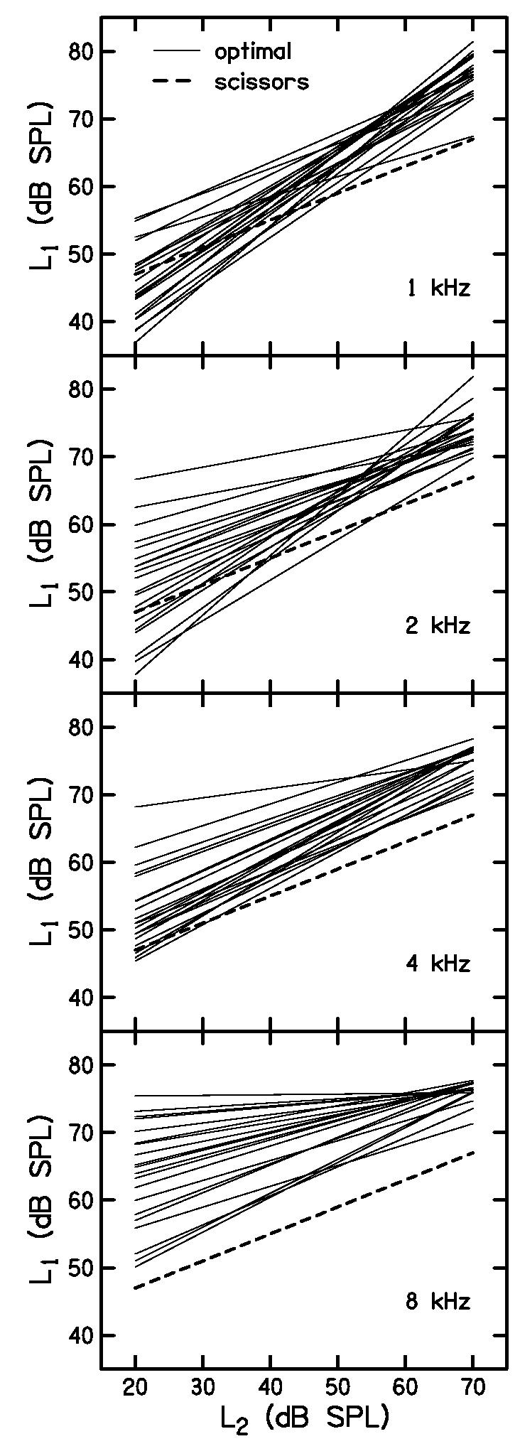
Optimal paths for all twenty subjects (thin, solid lines) are compared with the scissors path (thick, dashed line). Each panel shows data for a different f₂. This figure illustrates the distribution of the optimal paths across subjects at each frequency, as well their deviation from the scissors path.

These trends are summarized in Table I, which lists the average optimal path at each frequency, as well as an overall average for the present set of data. Because the optimal L₁ is greater than L₂ at low levels and its slope is less than one, there will be some value of L₂ for which L₁=L₂ will be optimal. That level is also listed in Table I under the heading equal. Finally, comparable values suggested by Kummer et al. (1998), Kummer et al. (2000), and Whitehead et al. (1995b) are also provided. The overall average in the present study is closer to the value reported by Whitehead et al. than it is to the values reported by Kummer et al. However, the present data suggest that there is a systematic effect of frequency, which is obscured in the average across frequency. Only the optimal, linear path at 2 kHz from the present study approximates the path recommended by Kummer et al.

Table I.

Coefficients of the optimal, linear path L₁ = a + b · L₂ averaged across all subjects at each frequency (kHz). The equal column indicates the stimulus level at which L₁=L₂. The linear fit suggested by Kummer et al. (1998) was based on the data of Gaskill and Brown (1990).

study	subjects	frequency (kHz)	a (dB SPL)	b	equal (dB SPL)
present	20	1	33	0.62	87
		2	42	0.46	77
		4	44	0.45	79
		8	58	0.26	78
		average	44	0.45	78
Whitehead et al. (1995)	8	3	45	0.5	90
Kummer et al. (1998)	5	average	39	0.4	65
Kummer et al. (2000)	22	average	41	0.41	70

C. I/O function comparisons

To assess the similarity between the I/O functions obtained with discrete-level and continuous-level stimuli, we examined the differences between I/O functions obtained by these two methods for both the scissors and optimal paths. Figure 8 shows the distribution of these differences in the first two boxes at each of four test frequencies. These data included all subjects and all values of L₂ for conditions in which the SNR was greater than 10 dB. Separate distributions of these differences are shown for the scissors path (vertical hatch) and optimal path (diagonal hatch). Thus, the first two boxes at each frequency compare the DPOAE levels for continuous and discrete presentation of the stimuli, holding constant the paradigm that was used to set stimulus level (scissors or optimal path). The boxes in Fig. 8 show the inter-quartile range (25^th to 75^th percentile) of the DPOAE level differences. The horizontal line through the middle of each box shows the median (50^th percentile) of the distribution. The fact that the scissors (vertical-hatch boxes) and optimal (diagonal-hatch boxes) are relatively short with medians near zero indicates that the I/O functions for continuous levels are similar to the I/O functions for discrete stimulus levels regardless of whether the levels are selected according to the scissor or optimal equation. Since the discrete-level method represents the standard approach for measuring DPOAE I/O functions, the similarity between DPOAE levels measured with these two methods validates the continuous-level method.

Figure 8.

Distribution (median and inter-quartile range) of DPOAE level differences at each frequency. The scissors (vertical hatch) and optimal (diagonal hatch) distributions compare the continuous-level measurement with the discrete-level measurement. These distributions are relatively narrow and centered near zero, indicating good agreement between the continuous-level and discrete-level measurements, especially for the optimal path. The distributions of differences between the optimal path and the scissors path for discrete-level stimuli (cross hatch) are also shown at each frequency. These distributions tend to be centered above zero, indicating higher DPOAE levels were measured for the optimal path, especially when f₂=8 kHz.

The cross-hatch boxes in Fig. 8 represent the distribution of DPOAE level differences when the optimal path is compared to the scissors path for measurements with discrete stimulus levels. In contrast to the first two boxes at each f₂, these boxes are relatively tall with medians always above zero, indicating that the optimal path produces larger DPOAE levels than the scissors path. The advantage of the optimal path increases as frequency increases and is greatest at 8 kHz, where the median difference in DPOAE level is about 10 dB. It is not surprising that the optimal path results in responses that are at least as large as those observed with the scissors path, since the stimulus levels used for the optimal-path measurements were, by definition, the levels that produced the largest DPOAE levels. However, the size and direction of the differences and the fact that these differences were observed in about 70% of the stimulus conditions at 1 and 2 kHz and 90-100% of the cases at 4 and 8 kHz suggests that the scissors path does not, on average, produce the largest DPOAEs in subjects with normal hearing. The DPOAE level differences when the optimal path is compared to the scissors path for measurements with continuous-level stimuli are not shown in Fig. 8, but are similar to the differences obtained with discrete-level stimuli.

D. Measurement time

One of the advantages that the continuous-level stimulus may offer over discrete-level stimuli is the time required to measure a DPOAE I/O function. The continuous-level paradigm includes a fixed amount of time, independent of the conditions of the measurement. Specifically, 262, 131, 66, and 66 seconds of data-collection time were used at 1, 2, 4, and 8 kHz, regardless of noise levels. Furthermore, this paradigm does not incorporate artifact rejection, so transient spikes potentially could be included in the response. In contrast, the time required to measure an I/O function using discrete-level stimuli may vary from condition to condition in the present study because measurement-based stopping rules controlled when each measurement was terminated. These rules allowed averaging to continue until either noise level was less than −25 dB SPL or the length of artifact-free averaging time was 32 seconds, whichever occurred first. Thus, the use of measurement-based stopping rules and the inclusion of artifact rejection potentially could increase the total discrete-level measurement time. These factors should be kept in mind when comparing the data-collection times for the continuous-level and discrete-level conditions.

The average time (across subjects) that was required to measure two scissors or two optimal path I/O functions using discrete-level stimuli is listed in Table II for each f₂ frequency. The discrete-level I/O functions were repeated for comparison with continuous-level stimuli, because the latter always produces two I/O functions, one for ascending levels and one for descending levels. On average, the time required to measure I/O functions using the discrete-level method was quadruple the time required for the continuous-level method.

Table II.

Average time (s) required for measurement of two I/O functions for each level variation method (discrete or continuous) at each frequency (kHz). For the discrete-level stimuli, the two I/O functions represent repeated conditions. For the continuous-level stimuli, the two I/O functions represent ascending and descending levels.

frequency (kHz)	discrete (s)	continuous (s)
1	999	262
2	601	131
4	340	66
8	272	66
average	553	131

The data-collection times listed in Table II should be interpreted in relation to the noise levels that were achieved by the continuous-level and discrete-level paradigms. That is, the advantage in averaging time for the continuous-level paradigm would not be impressive if it were achieved at the expense of a concomitant increase in noise levels. Table III compares the noise levels at each frequency for the two different paradigms. As can be seen in this table, the additional averaging time allowed the discrete-level measurements to achieve lower noise levels. The discrete-level noise levels were lower than those achieved by the continuous-level paradigm, ranging from 2.4 dB lower (at 1 kHz) to 6.9 dB lower (at 8 kHz), with an overall average that was lower by 4.2 dB. These results suggest that the data-collection time advantage of the continuous-level paradigm was essentially counterbalanced by the increased noise levels at 8 kHz (i.e., a four-fold decrease in averaging time would be expected to result in a 6-dB increase in noise level). However, at all other frequencies (and in the average across frequency), the reduced averaging time for the continuous-level paradigm did not result in an equivalent increase in noise level.

Table III.

Average noise level (dB SPL) for each level variation method (discrete or continuous) at each frequency (kHz). The averages include both scissors and optimal paths because the noise level was independent of stimulus level.

frequency (kHz)	discrete (dB SPL)	continuous (dB SPL)
1	−20.9	−18.5
2	−27.5	−24.3
4	−29.1	−24.5
8	−29.1	−22.2
average	−26.6	−22.4

E. Optimal versus scissors for discrete-level I/O functions

The discrete-level DPOAE I/O functions, averaged across subjects, are shown in Fig. 9. The thick line represents the mean DPOAE level at 2f₁-f₂ and the thin line represents the noise at this frequency. The format of Fig. 9 is similar to the one used in Fig. 5, with data from the scissors path on the left, optimal path on the right, and a different f₂ in each row. The error bars in Fig. 9 represent plus or minus one standard deviation from the mean for each L₂ from −5 to 80 dB SPL. Thus, the error bars in this figure represent variability for all of the data, including those conditions for which the SNR is low (L₂ ≤ 20 dB SPL). The dB value in each panel is the average standard deviation across the L₂ for which the SNR was greater than 10 dB. This, it represents an estimate of the inter-subject variability in DPOAE level, restricted to conditions where the response was reliably measured. The average level produced by the optimal-level path exceeds that observed for the scissor path, especially at 8 kHz, consistent with the distribution of DPOAE level differences shown in Fig. 8. Visual inspection of the functions and their associated error bars suggest that there is little difference in the variability that is observed across subjects. However, comparing the optimal path to the scissors path, we see that the average standard deviation always decreased, especially at 8 kHz. In other words, the variability averaged across L₂ tends to be less for the optimal path than for the scissors path. Stated another way, there is less inter-subject variability in DPOAE levels when individually determined optimal level paths are used, an effect that is most pronounced at the two f₂ frequencies for which the DPOAE-level advantage is greatest (4 and 8 kHz). Still, the differences are not large, suggesting that there are other sources contributing to inter-subject variability.

Figure 9.

Average DPOAE I/O functions for discrete-level measurements. The mean DPOAE level (thick line) and corresponding noise level (thin line) are shown for each f₂ frequency for both scissors (left column) and optimal (right column) paths. The error bars indicate one standard deviation from the mean. Dashed lines represent estimated system distortion based on cavity measurements. The dB values in each panel are the average of all standard deviations with SNR ≥ 10 dB.

One additional feature that appears to distinguish the optimal path from the scissors path is the similarity in the shape of the I/O functions across frequency. This feature can be observed directly in Fig. 9 and indirectly by noting the similarity in the slopes of the I/O functions shown in Fig. 10. The growth rate (dB/dB) in Fig. 10 was computed from the slopes of the I/O functions in Fig. 9. Greater emphasis should be placed on the slopes for L₂ levels greater than about 20 dB SPL, because the SNR was more favorable at these levels for both paradigms and, therefore, the results are considered more reliable. At levels below about 20 dB SPL, there was less separation between signal and noise, resulting in less confidence in our calculations of slope and, therefore, a more cautious assessment of slope estimates at these levels. The similarity in the optimal-path growth rates across frequency in Fig. 10 appears to be greater than that observed for the scissors path for L₂ levels ranging from 20 to about 65 dB SPL. Stated another way, the optimal-level path resulted in DPOAE I/O functions that were less dependent on frequency.

Figure 10.

DPOAE growth rate as a function of stimulus level for scissors (left) and optimal (right) discrete-level measurements. These growth rates are the slopes of the I/O functions shown in Fig. 9. The growth rate for the optimal path shows less variability across frequency compared to the scissors path.

The average phase of the I/O function across subjects was obtained by averaging complex pressure values at 2f₁-f₂, and is shown in the upper half of Fig. 11. Only measurements which had an individual SNR greater than 3 dB were included in the average. The lower half of Fig. 11 shows the vector strength (Goldberg and Brown, 1969) associated with each phase average. The line weights in Fig. 11 follow the convention used in Fig. 10. Just as we observed in the individual data shown in Fig. 6, the average DPOAE phase in Fig. 11 has a tendency to decrease with increasing stimulus level at all frequencies and for both scissors and optimal paths. The total decrease in phase tends to be about 0.5 to 1 cycles between 0 and 80 dB SPL, independent of frequency. This trend is observed despite low values of vector strength, which indicate broad distributions of individual phase values across subjects. The phase decrease for the scissors path (left panel) tends to be uniform across all levels, whereas, for the optimal path, the phase decreases more below 40 dB SPL than it does at higher levels. For the optimal path, there was little phase change between 40 and 60 dB SPL, except at 2 kHz, where the phase increased above 45 dB SPL. While the general trend was a decrease in phase with increasing stimulus level, regardless of the particular stimulus path, this result should be interpreted cautiously, given the variability across subjects suggested by the low vector-strength values.

Figure 11.

Average DPOAE phase (upper) and vector strength (lower) as a function of stimulus level for scissors (left) and optimal (right) discrete-level measurements. Different frequencies are represented by varying line widths. The complex pressure at 2f₁-f₂ was averaged across all subjects to obtain these phase values. To facilitate comparison, each phase curve has been unwrapped and shifted vertically so that its value would be zero at 40 dB SPL.

IV. DISCUSSION

The major findings from this study are (1) the development of a stimulus paradigm that allows one to explore a large L₁,L₂ space in a relatively short period of time, (2) validation of this technique by demonstrating the similarity in DPOAE levels obtained with it to the DPOAE levels obtained by more traditional measurement techniques at comparable stimulus levels, (3) demonstration that the optimal-level path depends on frequency, (4) demonstration that the optimal-level path results in larger responses than another commonly used paradigm for selecting stimulus level, and (5) that the DPOAE I/O functions are more similar across frequency and less variable across subjects when the optimal-level path is used, compared to the scissors path.

A. Analysis bandwidth

A 2-Hz bandwidth was selected for heterodyne analysis of the Lissajous-path responses because a smaller bandwidth would distort the shape of the Lissajous pattern formed by the primary levels and a larger bandwidth would decrease the SNR. This bandwidth was too small to allow accurate representation of DPOAE levels because these levels were changing so rapidly. In other words, the smoothing of the DPOAE level by the heterodyne analysis caused these levels to differ from those measured with discrete-level stimuli. However, because smoothing did not alter the locations of the most prominent DPOAE-level maxima in L₁,L₂ space, the Lissajous-path measurements retained sufficient information to determine an optimal path, despite the smoothing.

Possible evidence of excessive smoothing can be observed in the large deviation of some squares from the solid line in Fig. 2. The main reason for these large deviations was because DPOAE level tended to be larger during portions of the stimulus when L₁ and L₂ were both increasing. The dependence of DPOAE levels on the direction of stimulus level changes indicates that the stimulus levels were changing too rapidly to approximate steady-state conditions; however, this dependence was apparently exaggerated by the narrowness of the analysis bandwidth. Local maxima in DPOAE level were spread over a wider range as a result of smoothing. We observed that increasing the analysis bandwidth reduced the largest deviations of the squares from the solid line in Fig. 2; however, it was decided that the present amount of smoothing was acceptable and was selected because it provided better SNR than was provided by the larger bandwidth. Another way to reduce the influence of smoothing would have been to reduce the rate of stimulus-level changes, either by increasing the duration of stimulus or by reducing the number of cycles of level modulation. Both of these modifications to the stimulus have corresponding disadvantages and were not explored in the present study. Considering the alternatives, the 2-Hz analysis bandwidth appears to represent a reasonable compromise between competing needs. Still, the selection of analysis bandwidth for the Lissajous-path measurement warrants further consideration in future studies.

B. Frequency dependence

The data displayed in Fig. 7 suggest that the optimal, linear path for maximum DPOAE level depends on frequency, contrary to the suggestion of Kummer et al. (2000). The observation of frequency dependence, however, is perhaps not surprising. One might expect the optimal path to have a steeper slope at low frequencies because the basilar membrane (BM) excitation patterns for these stimuli overlap more than at high frequencies, resulting in more similar BM growth rates for the two tones at the site of DPOAE generation. The excitation patterns for higher frequencies with the same f₂/f₁ will be separated to a larger degree, which might result in more different growth rates at the DPOAE generation site. If the growth of BM response to f₁=6.7 kHz at the f₂=8-kHz place is more rapid than the f₁=0.83 kHz response growth at the f₂=1-kHz place, then the rate at which L₁ will need to increase to maintain the maximum interaction at the f₂ place will depend on frequency. Under these conditions, maintaining similar BM displacements at the generation site for the two tones requires L₁ to change level much more slowly than L₂ when f₂=8 kHz than when f₂=1 kHz. Presumably, this is why the optimal path has a shallower slope at high stimulus frequencies, compared to lower frequencies.

According to this view, one would predict an interaction between primary-level ratio and primary-frequency ratio. Thus, the frequency dependence of the optimal-path slope might be reduced by selecting a smaller f₂/f₁ ratio for higher frequencies. In this way, the relative overlap between the BM excitation patterns for f₁ and f₂ could be made to be more consistent across frequency. Stated another way, either decreasing f₂/f₁ or increasing L₁ can compensate for differences in frequency selectivity as a function of place along the basilar membrane. By decreasing f₂/f₁, the relative growth rates between the BM responses at the place of DPOAE generation would be more consistent. This consistency should be reflected in the slope of the optimal path. In support of this interpretation, Mills (2002) observed in gerbils that the f₂/f₁ producing the largest DPOAE levels decreases as f₂ increases.

C. Measurement time

The advantage of reduced measurement time for the continuous-level I/O function compared to the discrete-level I/O function, as shown in Table II, should also take into account the higher noise level for the continuous-level I/O functions listed in Table III. At 8 kHz, the increased noise levels essentially negated the benefit of the decreased data-collection time. While the continuous-level paradigm resulted in higher noise levels than the discrete-level paradigm at other frequencies, the increased noise level was less than would be predicted by the decreased data-collection time. If noise equivalency is a goal, we should be able to achieve similar noise levels with continuous-level measurements by doubling the measurement time at 1 and 2 kHz and quadrupling the measurement time at 4 and 8 kHz; however, this increase in measurement time would reduce its advantage over discrete-level measurements to less than a factor of two. An alternative way to achieve a similar noise floor with the continuous-level measurement would be to decrease the analysis bandwidth; however, this approach would lead to about 1 or 2 dB greater deviations from DPOAE levels measured with discrete-level stimuli. Considering the inescapable trade-offs among (1) measurement time, (2) noise level, and (3) DPOAE-level accuracy, the apparent advantage of the continuous-level measurement appears smaller than suggested by the times listed in Table II. However, continuous-level measurements may still be preferable to discrete-level measurements in some situations, especially when accuracy of DPOAE levels in less important, such as in the determination of the optimal, linear path. Another situation in which the continuous levels could offer a significant advantage over discrete levels is when the SNR is sufficiently high that the transient responses due to switching stimulus levels occupy a significant percentage of the averaging time required at each level. This may be the case in typical laboratory studies because the SNR is usually much greater in experimental animals than in humans, so avoiding transient-response time has a greater influence on total measurement time.

D. I/O function variability

The similarity across frequency of the DPOAE I/O function growth rates shown in Fig. 10 for the optimal path suggests that the optimal path reduces individual variability in I/O functions by compensating for individual-ear difference in the ear-canal geometry and/or middle-ear transmission. The compressive shape of the DPOAE I/O function is due to compressive growth of BM vibrations. The similarity of DPOAE growth across frequency suggests a corresponding similarity in BM growth across frequency. Individual differences in ear-canal and/or middle-ear characteristics could affect the relative levels of primary-tone responses within the cochlea and, as a consequence, cause the DPOAE growth rates to differ, despite consistency of BM growth rates for single tones. The use of optimal-path stimuli can compensate for these differences in individual ears. Variability across ears, however, cannot be completely attributed to level differences reaching the site of generation, because variability remained even after individualized optimal-level paths were used.

Similarity of the I/O functions across frequency provides evidence that the cochlear mechanisms that cause BM growth to be nonlinear have relatively invariant characteristics along the length of the cochlea, at least for the cochlear regions over which frequencies from 1 to 8 kHz are represented. The assumption of such invariance in BM growth has been used by Keefe (2002) to compute estimates of middle-ear forward and reverse transfer functions based on measurements of DPOAE I/O functions. Miller and Shera (2002) observed, however, that the I/O functions used by Keefe had fixed values of L₁ for each L₂ despite differing values of middle-ear forward transfer at f₁ and f₂. Consequently, the relative level of these two frequency components within the cochlea was not held constant across frequency. The fact that the optimal path I/O functions in the present study were less variable across frequency and across subjects suggests that relative levels within the cochlea were more consistent. Therefore, estimates of middle-ear transfer functions derived from individualized optimal-path I/O functions could be more accurate than those derived from I/O functions measured with any stimuli that have fixed level differences for all subjects. At the very least, the frequency effect described in the present study suggests that the DPOAE I/O functions obtained with a fixed primary-level ratio regardless of frequency may not provide the best data from which to derive estimates of forward and reverse energy transmission.

E. Optimal path

Our results indicate an optimal path through L₁,L₂ space, averaged over subjects and over stimulus frequency, is L₁ = 44 + 0.45 · L₂ . This result is consistent with previous recommendations to make L₁ > L₂ at low stimulus levels (Gaskill and Brown, 1990; Whitehead et al., 1995b; Kummer et al., 1998, 2000).

Whitehead et al. (1995b), based on measurements in 8 human subjects, suggested the use of L₁ = 45 + 0.5 · L₂ at 3 kHz, which is close to our optimal path when averaged across frequency. They also observed some frequency dependence to their optimal path by noting that the constant term was less (in the 32 to 42 dB range ) at other frequencies (both above and below 3 kHz) when the slope (0.5) was kept constant.

Our optimal path lies above the Kummer et al. (1998) scissors path L₁ = 39 + 0.4 · L₂ , which was based on the data of Gaskill and Brown (1990). According to our results, L₁ needs to be higher than the scissors path to obtain the largest DPOAE levels at each L₂. Kummer at al. (2000), based on measurements in 22 subjects, essentially confirmed their earlier recommendation for the optimum path, although they suggest a slightly higher path L₁ = 41 + 0.41 · L₂. Contrary to our results, they found little frequency dependence in their scissors path, although their methods were similar to ours. One possible reason for the discrepancy between their results and ours could be the more limited dynamic range of their stimuli. Their stimulus levels went no higher than L₁=70 and L₂=65 dB SPL. Their maximum measurement time of four seconds per stimulus condition also limited the minimum stimulus levels at which reliable measurements could be made (as evidenced by the SNR). However, the frequency effects described in Figs. 7 and 8 of the present paper are large. Therefore, differences in the range of stimulus levels may not be adequate to explain the differences between the present results and those described in Kummer et al. (2000).

The continuous-level method, which allows us to explore a large region of L₁,L₂ space in a relatively short amount of time, estimates the optimal path in less time than traditional methods. Although we have taken advantage of this method to provide average optimal paths at each frequency, as well as averaged across frequency, the preferred approach would be to use individual estimates of the optimal path for each ear. This is because current stimulus calibration methods, whether in-the-ear or in an acoustic cavity, are unable to guarantee that the desired level difference between the two tones will be achieved within the cochlea. Determining the individual optimal path in each ear provides the best way to maximize the DPOAE level as a function of stimulus level. While this approach might be preferable in normal-hearing subjects under laboratory conditions, the problem becomes more complex when measuring responses in possibly hearing-impaired subjects under clinical conditions. Here, the approach that is taken to select stimulus level probably will depend on the question that is being asked. If the aim is to distinguish ears with normal hearing from ears with hearing loss, then it might be more appropriate to select the average normal optimal-level path and apply those values with patients in the clinic. Although this path might not be optimal for individual hearing-impaired subjects (or for individual normal-hearing subjects), it might result in greater separation between the response distributions from normal and impaired ears, which is the goal in dichotomous clinical decisions. On the other hand, individual optimal-level paths might be more useful in clinical applications where the DPOAE I/O function will be used to predict behavioral threshold (Boege and Janssen, 2002; Gorga et al., 2003) or loudness growth (Müller and Janssen, 2004). Under these circumstances, selecting a stimulus path that takes into account any individual differences in calibration and/or energy transfer through the middle ear might provide a better estimate of BM response growth, which is the variable of interest when evaluating the relationship between DPOAE I/O functions and behavioral thresholds or loudness growth.

F. Level-dependent phase shift

It is of some interest that the same trend of decreasing phase with increasing level that was observed for a single subject in Fig. 6. is preserved in the average data from twenty subjects shown in Fig. 11. As stated above, we interpret the decrease in phase to indicate a shift in the place of DPOAE generation of about 1 cycle. The suggestion of a shift towards the base as level increases is not surprising, given the direction in which excitation spreads in the cochlea (e.g., Rhode and Recio, 2000). This result is also consistent with the upward spread of DPOAE suppression (Gorga et al., 2002), which similarly suggests that the place of DPOAE generation moves toward the base of the cochlea as stimulus levels increase.

Shera and Guinan (2003) have estimated that the wavelength of the BM response in a human cochlea is about 1.3 mm at 1 kHz, but decreases with increasing frequency at a rate of about 25% per octave. The level-dependent phase shift in the present study shows no such consistent trend with frequency over a three-octave range. This suggests that the level-dependent shift in the place of DPOAE generation is more likely to be consistent in terms of cycles than distance along the BM.

V. CONCLUSIONS

The Lissajous-path measurement using continuous-level stimuli provides an efficient method to determine an optimal, linear path that will usually produce larger DPOAE levels than more traditional approaches to setting primary levels, such as the Kummer et al. (1998) scissors path. In addition to producing larger DPOAE levels, the individualized optimal path produces I/O functions that are slightly less variable across subjects and slightly more consistent in shape across frequency. Consequently, DPOAE I/O functions measured with individualized optimal paths may yield more accurate predictions of hearing thresholds or loudness growth.

The optimal path differs across subjects and across frequency. The slope of the optimal path is steeper at low frequencies and less steep at high frequencies. This observation is consistent with direct observations of cochlear mechanics that show nonlinear BM growth more spatially distributed at low frequencies and more localized at high frequencies (Cooper and Rhode, 1995; Robles and Ruggero, 2001). Despite this clear variation in nonlinear growth characteristics across frequency, DPOAE I/O functions maintain a similar shape across frequency. This observation appears to be consistent with psychophysical data that show similar loudness growth across frequency (e.g., Fletcher and Munson, 1933; Müller and Janssen, 2004).

REFERENCES

- American National Standards Institute . ANSI S3.6. American Institute of Physics; 1996. Specifications for Audiometers. [Google Scholar]
- American Speech-Language-Hearing Association Guidelines for screening for hearing impairment and middle-ear disorders,” Working Group on Acoustic Immittance Measurements and the Committee on Audiologic Evaluation. ASHA. 1990;(Suppl 2):17–24. [PubMed] [Google Scholar]
- Boege P, Janssen T. Pure-tone threshold estimation from extrapolated distortion product otoacoustic emission I/O-functions in normal and cochlear hearing loss ears. J. Acoust. Soc. Am. 2002;111:1810–1818. doi: 10.1121/1.1460923. [DOI] [PubMed] [Google Scholar]
- Brown AM, Gaskill SA. Measurement of acoustic distortion reveals underlying similarities between human and rodent mechanical responses. J. Acoust. Soc. Am. 1990;88:840–849. doi: 10.1121/1.399733. [DOI] [PubMed] [Google Scholar]
- Cooper NP, Rhode WS. Nonlinear mechanics at the apex of the guinea-pig cochlea. Hear. Res. 1995;82:225–243. doi: 10.1016/0378-5955(94)00180-x. [DOI] [PubMed] [Google Scholar]
- Fletcher H, Munson WA. Loudness, its definition, measurement, and calculation. J. Acoust. Soc. Am. 1933;5:82–108. [Google Scholar]
- Gaskill SA, Brown AM. The behavior of the acoustic distortion product, 2f1-f2, from the human ear and its relation to auditory sensitivity. J. Acoust. Soc. Am. 1990;88:821–839. doi: 10.1121/1.399732. [DOI] [PubMed] [Google Scholar]
- Goldberg JM, Brown PB. Response of binaural neurons of the dog superior olivary complex to dichotic tonal stimuli: some physiological mechanisms of sound localization. J. Neurophysiol. 1969;32:613–636. doi: 10.1152/jn.1969.32.4.613. [DOI] [PubMed] [Google Scholar]
- Gorga MP, Neely ST, Ohlrich B, Hoover B, Redner J, Peters J. From laboratory to clinic: a large scale study of distortion product otoacoustic emissions in ears with normal hearing and ears with hearing loss. Ear Hear. 1997;18:440–455. doi: 10.1097/00003446-199712000-00003. [DOI] [PubMed] [Google Scholar]
- Gorga MP, Neely ST, Dorn PA, Dierking D, Cyr E. Evidence of upward spread of suppression in DPOAE measurements. J. Acoust. Soc. Am. 2002;112:2910–2920. doi: 10.1121/1.1513366. [DOI] [PubMed] [Google Scholar]
- Gorga MP, Neely ST, Dorn PA, Hoover BM. Further efforts to predict pure-tone thresholds from distortion product otoacoustic emission input/output functions. J. Acoust. Soc. Am. 2003;113:3275–3284. doi: 10.1121/1.1570433. [DOI] [PubMed] [Google Scholar]
- Harris FP, Lonsbury-Martin BL, Stagner BB, Coats AC, Martin GK. Acoustic distortion products in humans: Systematic changes in amplitude as a function of f2/f1 ratio. J. Acoust. Soc. Am. 1989;85:220–229. doi: 10.1121/1.397728. [DOI] [PubMed] [Google Scholar]
- Hauser R, Probst R. The influence of systematic primary-tone level variation L2 – L1 on the acoustic distortion product emission 2 f1 – f2 in normal human ears. J. Acoust. Soc. Am. 1991;89:280–286. doi: 10.1121/1.400511. [DOI] [PubMed] [Google Scholar]
- Kim DO, Dorn PA, Neely ST, Gorga MP. Adaptation of distortion-product otoacoustic emission in humans. J. Assoc. Res. Otolaryngol. 2001;2:31–40. doi: 10.1007/s101620010066. [DOI] [PMC free article] [PubMed] [Google Scholar]
- Janssen T, Kummer P, Arnold W. Wachstumsverhalten der Distorsionsproduktemissionen bei kochleären Hörstörungen,” or “Growth behavior of distortion-product emission in cochlear hearing-impairment,” Otorhinolaryngol. NOVA. 1995;5:34–46. in German. [Google Scholar]
- Kummer P, Janssen T, Arnold W. Level and growth behavior of the 2f1-f2 distortion-product otoacoustic emission and its relation to auditory sensitivity. J. Acoust. Soc. Am. 1998;103:3431–3444. doi: 10.1121/1.423054. [DOI] [PubMed] [Google Scholar]
- Keefe DH. Spectral shapes of forward and reverse transfer functions between ear canal and cochlea estimated using DPOAE input/output functions. J. Acoust. Soc. Am. 2002;111:249–260. doi: 10.1121/1.1423931. [DOI] [PubMed] [Google Scholar]
- Kummer P, Janssen T, Hulin P, Arnold W. Optimal L(1)-L(2) primary-tone level separation remains independent of test frequency in humans. Hear Res. 2000;146:47–56. doi: 10.1016/s0378-5955(00)00097-6. [DOI] [PubMed] [Google Scholar]
- Miller AJ, Shera CA. Using DPOAEs to measure forward and reverse middle-ear transmission noninvasively. Assoc. Res. Otolaryngol. Abs. 2002;769 [Google Scholar]
- Mills DM. Interpretation of standard distortion product otoacoustic emission measurements in light of the complete parametric response. J. Acoust. Soc. Am. 2002;112:1545–60. doi: 10.1121/1.1505021. [DOI] [PubMed] [Google Scholar]
- Müller J, Janssen T. Similarity in loudness and distortion product otoacoustic emission input/output functions: implications for an objective hearing aid adjustment. J. Acoust. Soc. Am. 2004;115:3081–91. doi: 10.1121/1.1736292. [DOI] [PubMed] [Google Scholar]
- Neely ST, Liu Z. Tech. Memo. Vol. 17. Boys Town National Research Hospital; Omaha, NE: 1993. EMAV: Otoacoustic emission averager. [Google Scholar]
- Neely ST, Stevenson R. Tech. Memo. Vol. 19. Boys Town National Research Hospital; Omaha, NE: 2002. SysRes. [Google Scholar]
- Rhode WS, Recio A. Study of mechanical motions in the basal region of the chinchilla cochlea. J. Acoust. Soc. Am. 2000;107:3317–32. doi: 10.1121/1.429404. [DOI] [PubMed] [Google Scholar]
- Robles L, Ruggero MA. Mechanics of the mammalian cochlea. Physiol. Rev. 2001;81:1305–1352. doi: 10.1152/physrev.2001.81.3.1305. [DOI] [PMC free article] [PubMed] [Google Scholar]
- Shera CA, Guinan JJ. Stimulus-frequency-emission group delay: A test of coherent reflection filtering and a window on cochlear tuning. J. Acoust. Soc. Am. 2003;113:2762–2772. doi: 10.1121/1.1557211. [DOI] [PubMed] [Google Scholar]
- Whitehead ML, McCoy MJ, Lonsbury-Martin BL, Martin GK. Dependence of distortion-product otoacoustic emissions on primary levels in normal and impaired ears. I. Effects of decreasing L2 below L1. J. Acoust. Soc. Am. 1995a;97:2346–2358. doi: 10.1121/1.411959. [DOI] [PubMed] [Google Scholar]
- Whitehead ML, Stagner BB, McCoy MJ, Lonsbury-Martin BL, Martin GK. Dependence of distortion-product otoacoustic emissions on primary levels in normal and impaired ears. II. Asymmetry in L1,L2 space. J. Acoust. Soc. Am. 1995b;97:2359–77. doi: 10.1121/1.411960. [DOI] [PubMed] [Google Scholar]