Object Type Recognition for Automated Analysis of Protein Subcellular Location

Abstract

The new field of location proteomics seeks to provide a comprehensive, objective characterization of the subcellular locations of all proteins expressed in a given cell type. Previous work has demonstrated that automated classifiers can recognize the patterns of all major subcellular organelles and structures in fluorescence microscope images with high accuracy. However, since some proteins may be present in more than one organelle, this paper addresses a more difficult task: recognizing a pattern that is a mixture of two or more fundamental patterns. The approach utilizes an object-based image model, in which each image of a location pattern is represented by a set of objects of distinct, learned types. Using a two-stage approach in which object types are learned and then cell-level features are calculated based on the object types, the basic location patterns were well recognized. Given the object types, a multinomial mixture model was built to recognize mixture patterns. Under appropriate conditions, synthetic mixture patterns can be decomposed with over 80 percent accuracy, which for the first time shows that the problem of computationally decomposing subcellular patterns into fundamental organelle patterns can be solved.

I. INTRODUCTION

A. Subcellular Location Pattern Recognition

A major goal of biological research in the coming decade, frequently captured under the heading of systems biology, is the construction of detailed models that accurately describe the workings of cells, tissues and organisms. Each cell type has a distinct proteome, the set of all proteins that it expresses, and an essential step towards model construction is the thorough characterization of all aspects of the proteomes of all cell types (the term proteomics is used to describe characterization of proteomes). One critical protein characteristic that is often overlooked in proteomics efforts is subcellular location, yet knowledge of the places within cells where each protein is found is critical to realistic model building.

The most common method for determining subcellular location is examination by human experts of fluorescence microscope images showing the distribution of fluorescently-tagged proteins. This subjective approach has a number of limitations. The assignment of descriptive terms to each protein pattern may differ from investigator to investigator and even for the same investigator from trial to trial. Further, the terms used (even when they are drawn from a standardized vocabulary such as the Genome Ontology) do not have sufficient complexity to capture the range of subtle differences in distribution that proteins can display. Lastly, visual examination of images for many proteins under many conditions is very labor intensive.

An alternative is to develop automated systems that can interpret fluorescence microscope images in terms of the subcellular patterns they display. We have previously constructed such systems and demonstrated that they can recognize the major subcellular patterns with high accuracy in images of cultured cells [1]. Further, we have shown that the performance of these systems is better than that of a human observer, in that the automated systems can efficiently discriminate patterns (or classes) that cannot be distinguished by visual examination [2]. Our best current systems achieve an accuracy of 92% on 2D images from ten classes [3] and 98% on 3D images from eleven classes [4].

B. SLF Features and the “Mixture Pattern” Problem

The most critical components of these systems we have previously described are sets of numerical features (Subcellular Location Features, or SLF) that capture the essence of the location patterns despite extensive variation in cell size, shape, and orientation [5]. The 2D features are well suited to characterize the patterns in the particular kinds of images for which they were developed. However, they are calculated at the level of each cell, and thus detailed information about the individual components of the cellular patterns is not captured. This presents a challenge when trying to recognize a pattern that is a mixture of two or more fundamental patterns, as, for example, in the case of a protein that localizes to both the Golgi complex and lysosomes. In such cases, the feature values for the mixed pattern are unlikely to be similar to the feature values of any of the constituent fundamental patterns. Therefore, for example, a classifier that has already been trained to recognize the patterns of Golgi and lysosomes would fail to recognize a mixed Golgi-lysosome pattern as either Golgi complex or lysosomes.

An alternative would be to train a separate classifier for every possible combination of fundamental patterns, which of course is not practical due to the number of possible combinations. Even if it were possible it would be of limited use because it would not yield any quantitative information about how much of the protein is in one organelle and how much in the other. A more suitable solution would be to have a classification scheme capable of recognizing components of patterns independently. We present here one approach to such a scheme using a two-stage learning system incorporating recognition of the objects that comprise subcellular patterns.

C. Object-based Image Modeling and Problem Statement

There has been extensive work on object-based image modeling, at first using predefined objects and subsequently using learned objects [6], [7]. The typical problem is: Given input images that contain one or more objects drawn from a certain number of classes, find and recognize the object classes. This is approached using a two-stage process consisting of learning the object classes and training a classifier to recognize them. The initial object learning is usually aided either by specifying a general parametric form for the object types or by specifying spatial primitives of which objects can be composed.

We are interested in solving a related problem arising in the context of images depicting subcellular location: Given input images drawn from two or more known image classes which each consist of some combination of unknown object classes, learn to recognize the image classes using the object classes. This requires adding a third stage in which a classifier is trained to recognize the image classes given the object classes, and possibly using the image labels to influence the object learning in the first stage. Since proteins may be found in more than one subcellular organelle or structure (as discussed above), it is also critical to be able to solve a second related problem: Given input images drawn from two or more known fundamental image classes which each consist of some combination of unknown object classes, learn to use the object classes to decompose an input image into fractions of the fundamental classes of which it is composed.

D. Overview of Object Type Recognition

In the next several sections of this paper, we present the details of the two-stage approach and its application on recognizing either fundamental or mixed location patterns. Fig. 1 shows the overall approach and the section of this paper in which each step is described. Two classifiers are required, one to classify objects for object type recognition and the other to classify cells for fundamental pattern recognition. We refer to these in this paper as the object level classifier and the cell level classifier respectively.

Fig. 1.

The overall frame of object type recognition. The corresponding section of this paper is shown in parentheses

II. Image Dataset

To develop and test the two-stage approach, we have used a collection of 2D fluorescence microscope images previously used to develop and test methods for recognizing patterns at the whole cell level [5]. The collection was made on a cultured human cell line, HeLa cells, grown at low density so that cells were in general well separated from each other and images of single cells could easily be collected. It was collected at high resolution (100x objective), with each pixel corresponding to 0.23 μm by 0.23 μm in the sample plane. The fluorescent probes used were chosen to include all major organelles and to include pairs of similar pattern classes so that the sensitivity of various features and classifiers could be tested. Representative images for the 10 pattern classes are shown in Fig. 2. The numbers of images available for each class range from 73 to 98. For each protein image, a parallel DNA image was collected using a different fluorescent probe. The parallel DNA images allow comparison of the distribution of each protein to a common frame of reference.

Fig. 2.

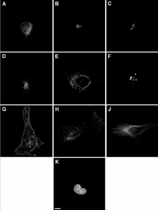
Representative images from the 2D HeLa image collection. The image classes represent the distributions of (A) an endoplasmic reticulum (ER) protein, (B) the Golgi protein giantin, (C) the Golgi protein GPP130, (D) the lysosomal protein LAMP2, (E) a mitochondrial protein, (F) the nucleolar protein nucleolin, (G) the filamentous form of the cytoskeletal protein actin, (H) the endosomal protein transferrin receptor, (J) the cytoskeletal protein tubulin, and (K) the fluorescent probe DAPI bound to DNA. Scale bar = 10 μm. From reference [5].

III. Objects and Object Types

A. Object Definition and Detection

Generally speaking, any part of the image can be viewed as an object. For our localization pattern analysis application, we give more interest to the regions with high intensity level, which correspond to the regions containing high concentrations of proteins (or DNA) tagged with fluorescence probes. Therefore, an object is defined as a continuous image region with above-threshold pixels. This definition does not attempt to ensure correspondence to physically separate objects in the sample, which may be overlapping and appear as a single object in the image. We were not overly concerned about this problem in our initial work since the high resolution imaging separates many object types (but this will be an area for future work).

The object detection was accomplished using automated threshold selection [8] and connected component detection using 8-neighbor connectivity. This process was identical to the object finding used to calculate average object features in our prior work [5]. There were over 61,000 objects detected in the 862 images in the 2D HeLa collection.

B. 2D Object-level Features

In order to be able to separately recognize the individual components comprising a subcellular pattern, a set of 11 features was calculated for each object (Table I). By analogy to our practice for Subcellular Location Features, we use the term Subcellular Object Feature (SOF) to refer to these features and define this set as SOF1.

TABLE I.

Features Used to Describe Subcellular Objects

Index	Feature Description
SOF1.1	Number of pixels in object
SOF1.2	Distance between object Center of Fluorescence (COF) and DNA COF
SOF1.3	Fraction of object pixels overlapping with DNA
SOF1.4	A measure of eccentricity of the object (see below)
SOF1.5	Euler number of the object
SOF1.6	A measure of roundness of the object (see below)
SOF1.7	The length of the object’s skeleton
SOF1.8	The ratio of skeleton length to the area of the convex hull of the skeleton
SOF1.9	The fraction of object pixels contained within the skeleton
SOF1.10	The fraction of object fluorescence contained within the skeleton
SOF1.11	The ratio of the number of branch points in skeleton to length of skeleton

Features 4 and 6 were defined as previously for cell classification [5], except of course they were calculated per object, not per cell. Features 2 and 3 are intended to describe each object in terms of its position within the cell and the rest are morphological descriptors. All feature values were normalized to z-scores (zero mean and unit standard deviation) across the entire object population.

C. Learning Object Types

The problem of recognizing image class from objects would be greatly simplified if a simple correspondence existed between image class and object types (as reflected by their features). This would permit training an object classifier using the label of the image each object is found in. However, this is not possible in our case for two reasons. The first is that some image classes contain objects of widely varying size and shape (making training potentially difficult). The second and more important reason is that some classes contain objects that are quite similar. For example, the endosomal, lysosomal, ER and mitochondrial patterns all contain small objects consisting of only a few pixels.

Therefore, we used two unsupervised learning approaches to define object classes. In the first, the objects from all 10 classes were clustered in the 11-dimensional feature space using the batch k-means algorithm, which is especially suitable for such large amounts of data because of its fast speed compared to other clustering methods. A Euclidean distance metric was used for clustering and k, the number of clusters, was chosen by trying all values of k from 1 to 40 in ten trials and using the Akaike Information Criterion (AIC) to judge which value was best. This is similar to the approach used by Ichimura [9], except both clustering and AIC were performed using Euclidean distance to allow clustering with small number of objects. Fig. 3 shows the relationship between AIC and k. While the graph shows a fairly shallow minimum, we conclude that the subcellular location patterns are basically composed of approximately 15–25 different types of objects. Since the AIC minimum occurred at 19, we used this value for further work. The dependence of classification accuracy on k will be discussed later.

Fig. 3.

Unsupervised learning of object types. Objects from all 862 images were clustered in the 11-dimensional SOF1 feature space using the k-means algorithm for various values of k. The average Akaike Information Criterion (AIC) over 10 trials for each k is shown.

The second approach we used for learning object types was to cluster the objects in each cell-level class. The optimal number of object clusters was found by AIC for each class, and ranged from 2 to 14. The final set of clusters was formed by combining the clusters from each of the classes. We term this method classwise clustering because the clustering is done class by class.

Having learned the clusters of basic object types, the object level classifier can be trained on these clusters to recognize the type of any given object. For the objects defined by clustering all classes together, object classification was done using a nearest centroid classifier (NCC), which classifies each object into the cluster whose centroid has the smallest Euclidean distance to the object. This is consistent with the clustering step, which also partitioned the training set according to distance to the centroids. For objects obtained for classwise clustering, the clusters from different classes may not be well separated by Euclidean distance, and therefore an NCC classifier is not suitable to assign an object from a test image to a cluster. Instead, we used a Linear Discriminant Analysis (LDA) classifier, which is based on the Mahalanobis distance, as the object level classifier. LDA requires the number of objects in the training set in each class to be no less than the number of features, so we merged any cluster that did not satisfy this condition into its closest cluster. This resulted in from about 40 to 3000 objects per cluster.

IV. Cell-Level Feature Sets

To recognize the pattern of a cell, information on objects in a cell should be converted to numerical features of the whole cell. A number of options of using the object assignments to generate features were considered.

An obvious way to differentiate patterns is to see if they have different frequencies of objects in each type. So the simplest cell-level feature set we chose was a vector of the number of each of the object types.

One problem with this feature set is that dim objects and bright objects have the same influence on the classification despite the fact that an object with more fluorescence makes a larger contribution to the cell-level pattern. Therefore, a second cell-level feature set was formed by the combination of the object number feature set and an additional feature vector of the fraction of total cell fluorescence contained in each type.

This set does not include any of the information contained in the individual object features, which might improve cell level classification. Therefore, a third cell-level feature set was defined to include all of the features above plus the average value of each SOF1 feature over all objects of each type in a cell. The total number of cell-level features in this set is thus 13k, where k is the number of object types. Due to the possible presence of correlated or uninformative features, which often exist in a cluster with small variance, such a large number of features can hinder the training of the classifier. Therefore we explored whether feature reduction would improve classification accuracy. We have previously evaluated eight methods for feature reduction, and observed that stepwise discriminant analysis (SDA) performed the best when both performance and computational cost were considered [10]. We therefore applied SDA to the features to select an informative subset. This subset was chosen for each object type method.

V. Mixture Pattern Recognition

A. Unmixing by Linear Regression

One motivation for clustering the objects into types is to solve the problem of recognizing mixture patterns. After object type learning, each fundamental pattern can be represented by a vector of either frequency of objects of k types or fraction of fluorescence in objects of k types. We construct feature matrix A by combining these vectors of all fundamental patterns along columns. A mixture pattern can be represented by a vector of mixture coefficients, α = (α₁, α₂,..., α_m)^T, where m is the number of fundamental patterns. We can then assume that the features of the mixture pattern, y = (y₁, y₂,..., y_k)^T, are linear combination of the features of fundamental patterns. For example, the mixture of pattern 1 with n1 objects of one type and pattern 2 with n2 objects of the same type simply generates a pattern with n₁ + n₂ objects of that type. So the task of mixture pattern decomposition is to solve the coefficients of the linear equationy = Aα

From our data, the row vectors in A are all linearly independent, which results in more equations than unknown variables to solve (k > m) and no guaranteed exact solution of the equation. A common way to deal with this problem is to solve the equation approximately by minimizing $\sum _{i=1}^k{(y_i-{\widehat{y}}_i)}^2$, where $\widehat{y}=A\widehat{\alpha }$ and $\widehat{\alpha }={({\widehat{\alpha }}_1,{\widehat{\alpha }}_2,\dots ,{\widehat{\alpha }}_m)}^{\text{T}}$. This results in the solution $\widehat{\alpha }={\left(A^{\text{T}}A\right)}^{-1}{A}^{\text{T}}y$. But the solutions do not necessarily satisfy ${\sum }_{u=1}^m{\widehat{\alpha }}_u=1$ and $0\le {\widehat{\alpha }}_u\le 1\mathrm{\hspace{0.17em} }\text{for\hspace{0.28em}}u=1,2,\dots ,m$. To get valid coefficients, we repeat the following steps until there is no negative coefficient: 1) Set all negative coefficients to 0 and remove the corresponding components; 2) Solve the new equation and then go to step 1. Finally all the coefficients are normalized to make sure that the sum is 1. The meaning of the coefficients changes with how A and y is defined. If A and y are defined using the fraction of number of objects in each pattern, then $\widehat{\alpha }$ is the fraction of objects in each component. Alternatively, if A and y are the fraction of fluorescence in each object type, $\widehat{\alpha }$ is the fraction of total fluorescence in each component of the mixture pattern.

B. Multinomial approach

As an alternative, the multinomial distribution can be used to describe each pattern because the features are counts of discrete categories. However, the number of objects in a cell is not a constant even in the same pattern. This means that the cells of the same pattern can not be represented by the same multinomial distribution. So it is more reasonable to assume that cells from the same pattern are generated by the same multinomial trials process except that the number of trials is varied from cell to cell. By assuming that all objects are independent and ignoring the number of trials, each pattern can be represented by k parameters θ_ul,..., θ_uk if there are k types of objects, where u is a label for the pattern and θ_ut is the probability that an object from pattern u belongs to type t. The parameters can be estimated as the percentage of the types in the training set, i.e. ${\widehat{\theta }}_{ut}=n_{ut}/n_t$, where n_ut is the number of objects belonging to type t in pattern u and n_u is the total number of objects in pattern u.

Any mixture pattern originating from m fundamental classes can be represented by another multinomial process with parameters

$$\sum _{u=1}^m{\alpha }_u{\theta }_{u1},\sum _{u=1}^m{\alpha }_u{\theta }_{u2},\dots ,\sum _{u=1}^m{\alpha }_u{\theta }_{uk}$$

where α₁, α₂,..., α_m, are unknown coefficients to estimate. This means that the probability that an object belongs to type t is ${\sum }_{u=1}^m{\alpha }_u{\theta }_{ut}$. We used the method of maximum likelihood to estimate the coefficients.

The likelihood function of the objects from a mixture pattern is

$$L=\prod _{i=1}^n\left(\sum _{u=1}^m{\alpha }_u{f}_u(x_i)\right),$$ (1)

where x_1, x_2, ..., x_n, are observed objects and f_u(x_i) = θ_ut if x_i belongs to type t.

The estimates ${\widehat{\alpha }}_1,{\widehat{\alpha }}_2,\dots ,{\widehat{\alpha }}_m$, are values maximizing the likelihood function, which is denoted as $({\widehat{\alpha }}_1,{\widehat{\alpha }}_2,\dots ,{\widehat{\alpha }}_m)=\underset{({\alpha }_1,{\alpha }_2,\dots ,{\alpha }_m)}{\text{arg\hspace{0.28em}max\hspace{0.28em}}L}$. Each of these values represents the percentage of objects from each fundamental pattern. It is difficult to get solutions analytically, so an iterative numerical method was used to search for solutions. Since the sum of the coefficients must be 1, the free parameters to be estimated are $({\widehat{\alpha }}_1,{\widehat{\alpha }}_2,\dots ,{\widehat{\alpha }}_{m-1})$, without ${\widehat{\alpha }}_m$, which is substituted by $1-{\sum }_{u=1}^{m-1}{\widehat{\alpha }}_u$. Maximizing L is the same as maximizing log L , which is denoted as l here. So the solutions are

$$({\widehat{\alpha }}_1,{\widehat{\alpha }}_2,\dots ,{\widehat{\alpha }}_{m-1})=\underset{({\alpha }_1,{\alpha }_2,\dots ,{\alpha }_{m-1})}{\text{arg\hspace{0.28em}max\hspace{0.28em}}L}=\underset{({\alpha }_1,{\alpha }_2,\dots ,{\alpha }_{m-1})}{\text{arg\hspace{0.28em}max\hspace{0.28em}}l}.$$ (2)

The first order derivative of l is

$$\begin{array}{l}\nabla l={\left(\frac{\partial l}{\partial {\alpha }_1},\frac{\partial l}{\partial {\alpha }_2},\dots ,\frac{\partial l}{\partial {\alpha }_{m-1}}\right)}^{\text{T}},\mathrm{\hspace{0.17em} }\text{where}\\ \frac{\partial l}{\partial {\alpha }_u}=\sum _{i=1}^n\frac{f_u(x_i)-f_m(x_i)}{{\sum }_{j=1}^{m-1}{\alpha }_j{f}_j(x_i)+(1-{\sum }_{j=1}^{m-1}{\alpha }_j)f_m(x_i)},\end{array}$$ (3)

and the Hessian matrix H of l is

$$\begin{array}{l}\left(\begin{array}{ccc}\frac{{\partial }^{2}l}{\partial {\alpha }_1^2}& \cdots & \frac{{\partial }^{2}l}{\partial {\alpha }_1\partial {\alpha }_{m-1}}\\ ⋮& \ddots & ⋮\\ \frac{{\partial }^{2}l}{\partial {\alpha }_{m-1}\partial {\alpha }_1}& \cdots & \frac{{\partial }^{2}l}{\partial {\alpha }_{m-1}^2}\end{array}\right)\\ =-\sum _{i=1}^n\frac{\left(\begin{array}{c}{f}_1(x_i)-f_m(x_i)\\ ⋮\\ f_{m-1}(x_i)-f_m(x_i)\end{array}\right){\left(\begin{array}{c}{f}_1(x_i)-f_m(x_i)\\ ⋮\\ f_{m-1}(x_i)-f_m(x_i)\end{array}\right)}^{\text{T}}}{\left({\sum }_{j=1}^{m-1}{\alpha }_j{f}_j(x_i)+(1-{\sum }_{j=1}^{m-1}{\alpha }_j)f_m(x_i)\right)}\end{array}.$$ (4)

This is a semi-negative definite matrix, which means that the log-likelihood l is a concave function. Therefore the global maximum of l can be found by Newton’s method or gradient ascent. Usually Newton’s method is faster than the gradient ascent method. The Newton’s method searches for the solutions by starting with initial values, which are $({\widehat{\alpha }}_1^{(0)},{\widehat{\alpha }}_2^{(0)},\dots ,{\widehat{\alpha }}_{m-1}^{(0)})=(\frac{1}{m-1},\frac{1}{m-1},\dots ,\frac{1}{m-1})$ here. At the 1 + r step of the Newton’s method, we have

$$\begin{array}{l}{({\widehat{\alpha }}_1^{(r+1)},{\widehat{\alpha }}_2^{(r+1)},\dots ,{\widehat{\alpha }}_{m-1}^{(r+1)})}^{\text{T}}\\ ={({\widehat{\alpha }}_1^{(r)},{\widehat{\alpha }}_2^{(r)},\dots ,{\widehat{\alpha }}_{m-1}^{(r)})}^{\text{T}}-H^{-1}\nabla l{|}_{({\widehat{\alpha }}_1^{(r)},{\widehat{\alpha }}_2^{(r)},\dots ,{\widehat{\alpha }}_{m-1}^{(r)})}.\end{array}$$ (5)

But from (5), we know that it needs the Hessian matrix to be non-singular or invertible.

Because f_u(x_i) = θ_ut if x_i belongs to type t, from (4) we have

$$H=-\sum _{t=1}^k\frac{n_i\left(\begin{array}{c}{\theta }_{1t}-{\theta }_{mt}\\ ⋮\\ {\theta }_{m-1t}-{\theta }_{mt}\end{array}\right){\left(\begin{array}{c}{\theta }_{1t}-{\theta }_{mt}\\ ⋮\\ {\theta }_{m-1t}-{\theta }_{mt}\end{array}\right)}^{\text{T}}}{{\left({\sum }_{j=1}^{m-1}{\alpha }_j{\theta }_{jt}+(1-{\sum }_{j=1}^{m-1}{\alpha }_j){\theta }_{mt}\right)}^2}.$$ (6)

Since H is the sum of k matrices with rank 1, the rank of H is no more than n, i.e. H is singular while k is less than m − 1. Therefore the total number of types of the objects of the mixture data must be greater than the number of fundamental patterns minus 2 to make H invertible. This was true in our application (k ≥ 19 and m = 10). If H is not invertible, the gradient ascent method can be used to search for the solution.

In our implementation, if a coefficient is smaller than a threshold (set to 0.1 divided by the number of objects) during estimation, it will be set to zero, which means that that component is not present.

VI. Pattern Recognition Results

A. Model Development

Before attempting to properly decompose mixture patterns, we first built cell level classifiers to test if the fundamental patterns could be well recognized based on the cell-level feature sets introduced in section IV. This is important because recognition accuracies indicate how well basic patterns can be represented by the feature sets. The testing procedure was done by stratified ten-fold cross validation, in which the total data set was randomly partitioned into ten subsets with approximately equal size for each class. Then for each of ten trials, a different subset served as testing set and the remaining nine subsets were used to learn object clusters and train the object level classifier. The output of the object level classifier was then converted into cell-level features. These features were fed into the cell level classifier, which was a back-propagation neural network (BPNN) with 20 nodes in a single hidden layer. To train the BPNN, the training set was further divided into two subsets. The BPNN was trained using two-thirds of the training set until the network error on the remaining third subset reached a minimum. Classification results from the test set were then recorded. No provision for prior-distribution of each class was made because all of the classes have comparable sizes. Most algorithms were implemented using Matlab (The Mathworks, Inc. Natick, MA). Some functions for object detection were written in C. The SDA algorithm was done by the STEPDISC procedure of SAS (SAS Institute, Cary, NC, USA). The codes for k-means algorithm and BPNN were from the NETLAB library (available at http://www.ncrg.aston.ac.us/netlab/) for Matlab.

Having shown that the object-based models worked well for recognizing fundamental patterns, we next considered their use for unmixing mixture patterns. We simulated mixture patterns by randomly generating mixture patterns from the test set. We again used 10-fold stratified cross validation. The training data were used to learn object types. For each fold, a set of 100 mixture patterns were generated by three steps: (1) randomly decide which fundamental patterns are going to be included in each trial and then (2) randomly select one cell from the test set of each pattern, (3) combine the objects of these cells to form a synthetic object mixture. Each object of the mixture pattern was then classified. The accuracy was calculated by the percentage of the objects that are accurately recognized, which can be calculated by ${\sum }_{i=1}^m\text{min}({\alpha }_i,{\widehat{\alpha }}_i)$. The overall accuracy was the average of accuracy rates of all trials from the ten folds and 100 trials were carried out for each fold. It is expected that if there are more samples of the same mixture pattern to decrease the risk of outliers, we can get better results. We therefore also tested mixtures composed of two or more cells from each fundamental pattern.

B. Basic Pattern Recognition

Table II shows the classification results averaged across 10 cross-validation trials based on the three feature sets from 19 types. The average correct classification rate increased when more features are used. The best average classification accuracy (75%) was obtained from using a combination of number, fluorescence, and summarized object-level features. We interpret the improvement to be mainly due to the inclusion in the summarized SOF of information about the spatial distribution of objects that was not captured using number of objects and fraction of fluorescence alone. Table III shows the confusion matrix of classification based on this feature set. It is shown as percentages because all classes have comparable sizes. We also note that the two Golgi classes are still difficult to distinguish, as we might expect since these are indistinguishable by visual examination [2]. If these two classes are merged, we obtain an average accuracy of 82% for the nine major patterns present in the 2D HeLa collection.

TABLE II.

Classification Results for Fundamental Patterns. The Object Level Classifier Was an NCC on 19 Clusters Using the 11 Object Features. The Cell Level Classifier Was a BPNN on One of the Three Cell-level Features: A. Number of Objects, B. Number of Objects and Fluorescence Fraction, C. Number of Objects, Fluorescence Fraction and Summarized Object-level Features. For the Last Feature Set, SDA was Applied to Select Best Features. So Number of Features Varies across Trials (57–70). (UA: Users accuracy; PA: Producers accuracy; OA: Overall accuracy.)

		Class
Feature Set		DNA	ER	Giant	GPP	LAMP	Mito.	Nucle.	Actin	TfR	Tubul.	OA(%)	KAPPA
A	UA(%)	83	63	52	54	60	60	77	77	68	59	66	0.62
PA(%)	100	72	18	82	67	36	81	82	55	64
B	UA(%)	84	69	58	53	66	62	83	81	69	69	70	0.67
PA(%)	100	76	39	62	67	49	86	82	62	75
C	UA(%)	95	77	63	59	67	80	87	91	67	67	75	0.72
PA(%)	99	88	49	60	68	59	91	91	62	82

TABLE III.

Classification Results for Summarized Object Features. The Object Level Classifier Was an NCC on the 11 Object Features. The Cell Level Classifier was a BPNN on 57–70 Features Selected from the 247 Cell-level Features by SDA. The Values Are the Percentage of Images in Each True Class That Are Classified in Each Output Class. The Overall Correct Classification Rate Was 75% (82% After Merging the Two Golgi Classes)

	Output of the Classifier
True Classification	DNA	ER	Giant	GPP	LAMP	Mito.	Nucle.	Actin	TfR	Tubul.
DNA	99	1	0	0	0	0	0	0	0	0
ER	0	88	0	0	3	0	0	0	1	7
Giantin	0	0	49	40	2	0	3	0	5	0
GPP130	0	0	27	60	6	0	6	0	1	0
LAMP2	1	4	2	0	68	0	2	0	21	1
Mitoch.	0	7	0	0	3	59	0	5	1	25
Nucleolin	5	0	0	0	4	0	91	0	0	0
Actin	0	0	0	0	0	3	0	91	1	5
TfR	0	9	0	0	14	3	1	3	62	8
Tubulin	0	7	0	1	0	5	0	2	2	82

Although including summarized object-level features results in better cell-level classification accuracy, there are advantages in having a feature set consisting of only object numbers. These include simplicity of building generative models and ease of unmixing combined patterns. We therefore sought ways to improve the discriminating power of the object types.

A simple approach could be to use more clusters. Fig. 4 shows classification accuracy as a function of the number of clusters obtained from k-means clustering. The accuracy from 19 clusters is close to the maximum accuracy (71%) in the figure. While the object clustering approach described above can help us find the statistically significant clusters, it does not guarantee that the clusters are optimal for classification based on object numbers. For example, two populations that are almost completely linearly separable might be merged into one cluster if they are close to each other in the feature space. Such a merge will assign the objects in the two distinguishable groups only to one type so that they will be unable to contribute to distinguishing the two classes they are derived from.

Fig. 4.

Cell-level overall classification accuracies for different numbers of clusters learned by batch k-means. The object level classifier was an NCC on the 11 object features and the cell level classifier was a BPNN on number of objects.

We therefore designed a classwise clustering approach to avoid this problem, as described in section III-C. Table IV shows the confusion matrix based on object types learned by classwise clustering. When the two Golgi classes were merged, the overall accuracy improved to 81%. This is nearly as high as the best performance (82%) we obtained so far (Table III), but it is important to note that it was achieved using only cluster membership as features. Comparison of Table II (feature set A) and Table V shows that using classwise clustering in the first stage improved the cell-level classification accuracy by an average of 6%. The largest improvements were in the mitochondrial and tubulin classes.

TABLE IV.

Classification Results for Object Types Learned by Classwise Clustering. The Object Level Classifier Was an LDA on 56–68 Clusters on The 11 Object Features. The Cell Level Classifier Was a BPNN Using the Number of Objects in Each Cluster As 56–68 Cell-level Features. The Overall Correct Classification Rate Was 72% (81% After Merging the Two Golgi Classes)

		Output of the Classifier
True Classification	DNA	ER	Giant	GPP	LAMP	Mito.	Nucle.	Actin	TfR	Tubul.
DNA	93	2	2	1	0	1	0	0	0	0
ER	0	69	0	1	5	2	0	0	6	15
Giantin	0	0	57	36	1	3	1	1	1	0
GPP130	0	0	39	55	5	0	0	0	1	0
LAMP2	0	2	5	7	56	0	0	0	26	0
Mitoch.	1	7	0	5	3	66	0	5	7	4
Nucleolin	0	4	5	1	1	0	88	0	1	0
Actin	0	1	0	0	0	2	0	88	1	8
TfR	0	5	1	0	14	10	0	0	64	5
Tubulin	0	4	0	1	0	8	0	1	1	85

TABLE V.

accuracy of Unmixing Synthetic Mixtures of Objects from Different Subcellular Location Patterns Using Linear Regression

A) Expressed as percentage of object correctly classified
	No. cells/pattern
	1	2	3	4	5
All	55	59	62	63	64
Merge Golgi	54	60	62	64	66
Merge Golgi, LAMP-TfR	58	63	67	68	68
B) Expressed as percentage of fluorescence in objects correctly classified
	No. cells/pattern
	1	2	3	4	5
All	64	70	72	74	74
Merge Golgi	70	74	76	77	78
Merge Golgi, LAMP-TfR	73	78	79	81	81

Another possible approach to improve the clustering is to use more features to describe each object, since the additional features create more chances of detecting significant differences between objects. We therefore added 13 texture features and 5 edge features because of their effective description of the patterns at the cell level [2], and defined this set as SOF2. The classwise clustering method was performed for the new feature set. Although it only resulted in a slight improvement in the average accuracy (from an average of 72% to 73%; data not shown), it turned out to be helpful for mixture pattern recognition.

C. Results of Mixture Pattern Recognition

As described above, we generated synthetic mixtures to test our ability to unmix patterns. Using the 11 SOF1 object features, the overall accuracy of unmixing obtained by linear regression was 39% for k-means clustering on 19 clusters and 50% for classwise clustering. The accuracy increased to 55% when SOF2 features were used in clustering. For the multinomial approach, the best overall accuracy of decomposition was also obtained from the clusters learned from the SOF2 features by classwise clustering (61%, vs. 40% and 57% for the other two clustering approaches). Therefore we used these clusters for our further experiments on mixture pattern recognition.

Table V shows the average mixture pattern recognition accuracies that were obtained when different numbers of cells were selected per pattern. There is significant improvement of performance of the decomposition with the increasing number of samples. When the decomposition was done as a fraction of fluorescence in each pattern, much higher accuracies were obtained than for fraction of object numbers. This is reasonable because the sum of square errors to minimize was no longer dominated by fundamental patterns with large number of objects. The accuracies can be further increased by merging confusing patterns, either just merging the two Golgi proteins to give nine classes, or also merging the LAMP and TfR classes to give eight classes.

The counterpart of results in Table V was calculated for the multinomial approach to compare this method with the linear regression. Table VI shows the average mixture pattern recognition accuracies that were obtained when different numbers of cells were selected per pattern. The accuracies increased with the number of cells. If we merged the two pairs of confused patterns, giantin-GPP130 and LAMP-TfR, the average decomposition accuracy increased to 76% when 5 cells per pattern was used for trials. As we observed for the results of linear regression, when the accuracy is expressed as a fraction of fluorescence in each pattern (Table VI-B), the accuracy rises to 83% for five cells drawn from each of the eight major patterns. These results would be expected to be comparable to those obtained from a corresponding number of cells showing a real mixture pattern.

TABLE VI.

Accuracy of Unmixing Synthetic Mixtures of Objects from Different Subcellular Location Patterns Using Multinomial Models

A) Expressed as percentage of object correctly classified
	No. cells/pattern
	1	2	3	4	5
All	61	65	69	71	72
Merge Golgi	63	68	71	72	74
Merge Golgi, LAMP-TfR	66	70	72	74	76
B) Expressed as percentage of fluorescence in objects correctly classified
	No. cells/pattern
1	2	3	4	5
All	66	71	73	74	76
Merge Golgi	70	75	78	79	80
Merge Golgi, LAMP-TfR	74	79	81	82	83

VII. Summary and Discussion

The work described here addresses the difficult task of extending a system that recognizes different classes of scenes (cells) to recognize new scenes comprised of mixtures of objects from the original scenes. The problem is made more difficult in this case because the number of allowed combinations is not known in advance. As an initial approach, cluster analysis was used to discover the fundamental types of objects present in 2D cell images and to show that sufficient information is retained in the individual objects so that they can be used to recognize the image class they were derived from with reasonable accuracy. Whereas the individual cell classification accuracy was not quite as high as obtained previously for cell-level classification of 2D images, it was high enough to encourage further work. As we have demonstrated previously, the cell-level accuracy can be increased dramatically if images of more than one cell are available [5].

We next extended the object learning approach to build systems that for the first time can analyze mixed organelle patterns by quantitatively decomposing them into fundamental patterns. We also found, as expected, that the results could be improved by using information from more than one cell. The ability to do mixture decomposition will be critical in the next few years to support efforts to collect and analyze subcellular location images on a proteome-wide basis [11]–[14]. While the patterns used for our initial studies were chosen to represent “fundamental” classes, we know that many proteins in future images will be present in more than one structure or organelle. Thus, the work described here can be used to determine the fraction of each protein that is found in various organelles and to monitor how those fractions change under various conditions, such as in the presence of drugs or disease.

Although the mixture models described here were built using a feature set of object numbers, they can be extended to any feature set. All that is needed is a way to estimate the statistical distribution of the features and an approach to find the maximum likelihood estimates. It is hard to derive a parametric distribution for high dimensional features. Fortunately, many nonparametric methods have been developed. The advantage of these methods is that they do not require any prior assumptions about the data distribution. Therefore, we can potentially make use of any feature set that is good for classification for mixture pattern recognition.

Without a statistical distribution of object features, the model can still be improved by using a more appropriate clustering method for object learning. Although the k-means algorithm using Euclidean distance is easily implemented and fast, it only works best for clusters with spherical shapes. In the future, we plan to try clustering methods that have more flexible separation boundaries to separate clusters, such as clustering with minimal spanning trees [15].

Regardless of whether the features are computed on a per cell or a per object basis, the feature values are totally dependent on the definition of what an object is. It is easy to define an object as a continuous region of pixels that are above a certain threshold, as we have here. However, in the case of a filamentous protein such as tubulin it might be desirable to define each filament as an object. With the simple definition used here, the tubulin pattern of a cell typically contains just one large mesh-like object because many tubulin filaments criss-cross throughout the cell. Therefore, we plan to explore more natural definition of objects in the future. For example, we can define an object as a region with uniform texture and then use texture extraction methods [16]–[18] to detect objects.

Figure legends

Based on our success at recognizing major patterns, we have previously extended this approach to unsupervised learning of many different protein patterns. This can be done by (1) generating high-resolution, fluorescence microscope images with all possible location patterns by randomly tagged all expressed proteins, and (2) using image analysis approaches to group proteins by their location patterns. We have used the term location proteomics to describe this new approach [14], [19]. The promise of location proteomics is to use discovery methods to create for the first time a complete understanding of the process by which proteins are localized in cells. The work described in this paper will provide an important new capacity, the ability to build object models from fundamental patterns. This will enable the description of every protein pattern using generative models, a critical component of systems biology approaches to modeling all aspects of cell behavior.

References

- 1.Huang K, Murphy RF. “From quantitative microscopy to automated image understanding,”. Journal of Biomedical Optics. SepOct 2004;9:893–912. doi: 10.1117/1.1779233. [DOI] [PMC free article] [PubMed] [Google Scholar]
- 2.Murphy RF, Velliste M, Porreca G. “Robust numerical features for description and classification of subcellular location patterns in fluorescence microscope images,”. Journal of VLSI Signal Processing Systems. 2003;35:311–321. [Google Scholar]
- 3.Huang K, Murphy RF. “Boosting accuracy of automated classification of fluorescence microscope images for location proteomics,”. BMC Bioinformatics. Jun 2004;5:78. doi: 10.1186/1471-2105-5-78. [DOI] [PMC free article] [PubMed] [Google Scholar]
- 4.X. Chen and R. F. Murphy, “Robust classification of subcellular location patterns in high resolution 3D fluorescence microscopy images,” in Proceedings of the 26th Annual International Conference of the IEEE Engineering in Medicine and Biology Society, San Francisco, CA, Sep. 2004, pp. 1632–1635. [DOI] [PubMed]
- 5.Boland MV, Murphy RF. “A neural network classifier capable of recognizing the patterns of all major subcellular structures in fluorescence microscope images of heLa cells,”. Bioinformatics. Dec 2001;17:1213–1223. doi: 10.1093/bioinformatics/17.12.1213. [DOI] [PubMed] [Google Scholar]
- 6.Cho K, Dunn SM. “Learning shape classes,”. IEEE Transactions on Pattern Analysis and Machine Intelligence. Sep 1994;16:882–888. [Google Scholar]
- 7.R. Michalski, A. Rosenfeld, Z. Duric, M. Maloof, and Q. Zhang, “Learning patterns in images,” in Machine Learning and Data Mining: Methods and Applications, R. S. Michalski, I. Bratko, and M. Kubat, Eds.: John Wiley & Sons, Ltd., 1998, pp. 241–268.
- 8.Ridler TW, Calvard S. “Picture thresholding using an iterative selection method,”. IEEE Transactions on System, Man and Cybernetics. Aug 1978;SMC-8:630–632. [Google Scholar]
- 9.Ichimura N. “Robust clustering based on a maximum-likelihood method for estimating a suitable number of clusters,”. Systems Computers Japan. Jan 1997;28:10–23. [Google Scholar]
- 10.Huang K, Velliste M, Murphy RF. “Feature reduction for improved recognition of subcellular location patterns in fluorescence microscope images,”. Proceedings of SPIE. 2003;4962:307–318. [Google Scholar]
- 11.Kumar A, Agarwal S, Heyman JA, Matson S, Heidtman M, Piccirillo S, Umansky L, Drawid A, Jansen R, Liu Y, Cheung KH, Miller P, Gerstein M, Roeder GS, Snyder M. “Subcellular localization of the yeast proteome,”. Genes & Development. Mar 2002;16:707–719. doi: 10.1101/gad.970902. [DOI] [PMC free article] [PubMed] [Google Scholar]
- 12.Ghaemmaghami S, Huh WK, Bower K, Howson RW, Belle A, Dephoure N, O'Shea EK, Weissman JS. “Global analysis of protein expression in yeast,”. Nature. Oct 2003;425:737–41. doi: 10.1038/nature02046. [DOI] [PubMed] [Google Scholar]
- 13.Jarvik JW, Fisher GW, Shi C, Hennen L, Hauser C, Adler S, Berget PB. “In vivo functional proteomics: Mammalian genome annotation using CD-tagging,”. BioTechniques. Oct 2002;33:852–867. doi: 10.2144/02334rr02. [DOI] [PubMed] [Google Scholar]
- 14.Chen X, Velliste M, Weinstein S, Jarvik JW, Murphy RF. “Location proteomics - Building subcellular location trees from high resolution 3D fluorescence microscope images of randomly-tagged proteins,”. Proceedings of SPIE. 2003;4962:298–306. [Google Scholar]
- 15.Zahn CT. “Graph-theoretical methods for detecting and describing gestalt clusters,”. IEEE Transactions on Computers. Jan 1971;C-20:68–86. [Google Scholar]
- 16.Khotanzad A, Chen JY. “Unsupervised segmentation of textured images by edge detection in multidimensional features,”. IEEE Transactions on Pattern Analysis and Machine Intelligence. Apr 1989;PAMI-11:414–421. [Google Scholar]
- 17.Buf JMHD, Kardan M, Spann M. “Texture feature performance for image segmentation,”. Pattern Recognition. 1990;23(34):291–309. [Google Scholar]
- 18.Chang KI, Bowyer KW, Sivagnurunath M. “Evaluation of texture segmentation algorithms,” in”. IEEE Conference on Computer Vision and Pattern Recognition. Jun 1999:294–299. [Google Scholar]
- 19.X. Chen and R. F. Murphy, “Objective clustering of proteins based on subcellular location patterns,” Journal of Biomedicine and Biotechnology, to be published, 2005. [DOI] [PMC free article] [PubMed]