

Abstract
The distributions of log-likelihood ratios (ΔLL) obtained from fitting ion-channel dwell-time distributions with nested pairs of gating models (Ξ, full model; ΞR, submodel) were studied both theoretically and using simulated data. When Ξ is true, ΔLL is asymptotically normally distributed with predictable mean and variance that increase linearly with data length (n). When ΞR is true and corresponds to a distinct point in full parameter space, ΔLL is Γ-distributed (2ΔLL is χ-square). However, when data generated by an l-component multiexponential distribution are fitted by l+1 components, ΞR corresponds to an infinite set of points in parameter space. The distribution of ΔLL is a mixture of two components, one identically zero, the other approximated by a Γ-distribution. This empirical distribution of ΔLL, assuming ΞR, allows construction of a valid log-likelihood ratio test. The log-likelihood ratio test, the Akaike information criterion, and the Schwarz criterion all produce asymmetrical Type I and II errors and inefficiently recognize Ξ, when true, from short datasets. A new decision strategy, which considers both the parameter estimates and ΔLL, yields more symmetrical errors and a larger discrimination power for small n. These observations are explained by the distributions of ΔLL when Ξ or ΞR is true.
INTRODUCTION
Conformational transitions of ion-channel proteins associated with gating are best described as a stochastic process governed by some discrete Markov model (1). Such models, called gating schemes, consist of sets of discrete open-channel and closed-channel conformations (states) connected to each other in a given pattern, and of rate constants which describe probabilities of transition along the allowed kinetic pathways. Many features of ion-channel gating, such as the durations of individual open- and closed-channel dwell times or the vector of the entire ordered sequence of open- and closed-time durations, are random variables whose distributions are defined by the underlying Markov model (2). These random variables can be experimentally sampled, as the timing of individual open-to-closed and closed-to-open transitions are observable in single-channel patch-clamp records (3). A steady-state current record of a single ion channel is first idealized to reconstruct the sequence of open and closed dwell times (the events list (2)) which is then fitted to an assumed gating scheme by maximum likelihood (ML) to obtain the set of parameters (rate constants, or time constants and fractional amplitudes of exponentials) which best describes the data—i.e., the set of dwell times (4), the set of pairs of consecutive open/closed dwell times (5), or the entire ordered series of dwell times (6–11).
Fitting pairs, or the entire series, of events reveals possible correlations between the durations of adjacent open and closed dwell times. Much valuable information has been obtained from such studies, e.g., for large-conductance Ca2+-activated K+ channels (5,12,13), several members of the pentameric ligand-gated ion channel family such as the glycine (14,15), the GABAA (16), and the nicotinic acetylcholine (17–19) receptor channel, and recently for the NMDA receptor (20). Nonetheless, traditional fitting of one-dimensional dwell times is still used to study channels for which such correlations are not apparent (21–25) or for which a gating scheme is not yet at hand (26,27); but also for a visual comparison of such fits with model predictions—even if the analysis itself relies on more sophisticated methods (12–16,18–20).
Typically, the true underlying gating scheme is unknown, and the aim of the experimenter is to find the minimal model that explains the experimental findings. Several possible models are therefore considered, and these are then ranked based on the likelihood, or its logarithm (Log-Likelihood, LL), of observing the data, given the model. When two models are compared that contain the same numbers of parameters, the one yielding a higher LL is accepted. Comparison of two models with different numbers of free parameters is more problematic, as more free parameters may result in slightly higher likelihood values even if the introduction of the additional parameters is not justified. A good strategy for model evaluation in this case depends on knowledge of the distribution of the log-likelihood ratio ΔLL = LL2 – LL1. The present work addresses this question for the subset of cases in which the model with fewer parameters is a submodel of the other (nested models). The results are presented in the framework of ML-fitting of one-dimensional dwell-time distributions; the implications for ML-fitting of joint distributions of series of dwell times are discussed. The core of the article consists of two basic parts—the first, more theoretically and the second, more practically oriented.
The section “Distributions of Log-Likelihood Ratios” investigates the distributions of ΔLL under various situations in which either the submodel or the broader model is the true model. For the case in which the broader model is true, the asymptotic distribution of ΔLL is mathematically derived and confirmed using extensive simulations. The case in which the submodel is true has been studied in the past (28) and is discussed in standard statistics textbooks (e.g., (29–31)); 2ΔLL is χ2-distributed if certain regularity criteria apply. This assumption has been widely used for evaluation of ion-channel gating schemes (e.g., (2,32)), but the applicability of the required regularity criteria to such models has not been tested. These criteria are examined here and shown not to apply in some of the most common situations. The empirical distributions of ΔLL for such cases are obtained from large sets of simulated data.
The section “Strategies for Model Discrimination” evaluates several existing methods for model identification, including the log-likelihood ratio test (LLR test, e.g., (32)), the Akaike information criterion (AIC, (33)) and the Schwarz criterion (SC, (34)). Experimenters often put their faith in these statistical tests without first studying the applicability of the underlying theorems. E.g., the assumptions required for use of the canonical LLR test frequently do not apply (a valid LLR test for such cases is presented here). Moreover, even studies in which these methods were tested on simulated data (6,7,9) have examined their efficiencies only under limited sets of conditions. First, the ability to detect an extra component in a distribution is very dependent on the size of that component. It is inevitable in simulation studies that the results depend on the chosen values of the rate constants. Second, the value of ΔLL is a random variable. Therefore, obtaining a correct decision for a single simulated events list may provide little information. For a given model, a large set of independent events lists should be examined to obtain a population of decisions that will allow estimation of the probabilities of error. Third, the effect of the length of the data on the reliability of the decision lacks systematic evaluation. E.g., for each of the above statistical tests the Type I error (rejection of the null hypothesis although it is true) and Type II error (acceptance of the null hypothesis although it is wrong) depend differentially on the length of the data.
These issues are explored here for nested pairs of models using large sets of simulated data, and the findings explained in light of the distributions of ΔLL for both cases, i.e., when the submodel is correct (the null hypothesis) and when it is incorrect. In addition, a new decision strategy is proposed, which is not a priori biased toward either of the two models and produces relatively symmetrical Type I and Type II errors. Because it also results in a higher power of discrimination for relatively small data sets, the novel approach might prove a useful alternative of the LLR test, and of the AIC or SC, for such applications.
MATERIALS AND METHODS
Simulations
Simulated sequences of dwell times (events lists) were generated as described (e.g., (35)), using exponentially distributed random numbers obtained by a transformation on an evenly distributed random variable (36). To minimize simulation-related artifacts, evenly distributed random numbers were generated using the high-quality random generator ran2 (36). This function combines a long-period random sequence algorithm (37) with a shuffling procedure (38) which further removes serial correlations. The period of ran2 is ∼2 × 10¹⁸, which allows generation of a random sequence of ∼1018 channel gating events, as each such event consumes two random numbers. For a given gating scheme, 1000 independent events lists of length 2n (containing n closed events) were produced by simulating one long events list of length 2000n, which was then broken up into 1000 parts of length 2n each. For the longest individual events lists studied, n was 104; thus, simulation of 1000 such events lists consumed 4 × 10⁷ random numbers, far smaller than the period of the generator.
Maximum likelihood fitting
Closed dwell times of simulated events lists were fitted to multiexponential probability density functions by unbinned ML (e.g., (4)). The LL was maximized with respect to the parameters of the fitted distribution using two optimizers, an uphill simplex algorithm (39) and the Davidon-Fletcher-Powell variable metric method (36), started from several different seed parameters. This was especially important when the fitted distribution contained more parameters than the true generating distribution. E.g., in the case in which single-exponentially distributed dwell times are fitted by a double-exponential distribution, the best unconstrained ML estimate  is expected to scatter in a broad region of the parameter space Ω (along a jointed line such as that depicted in Fig. 7). Thus, in such cases, each events list was fitted using both optimizer algorithms, both seeded from 40 different seed values along the expected jointed line. Out of the 80 parameters to which these attempts converged,
  was chosen as the one that yielded the highest LL. However, it must be noted that despite all the effort to identify the best
  it remains possible that for some of the events lists the true
  was not found. Single-exponential distributions were fitted by solving the likelihood equation; i.e., the ML estimate of the time constant was obtained as the arithmetic average of the dwell times.
FIGURE 7.

Full parameter space of the closed-time distribution of Scheme 2. The parameter space Ω is the subset of three-dimensional space bounded by τc1 ≥ 0, τc2 ≥ τc1, acl ≤ 0, and acl ≤ 1. The reduced space ΩR, which describes Scheme 2R, is a one-dimensional line in Ω (see Fig. 3 F), defined, e.g., by the constraints τc2 = τc1, and acl = fixed (to any value). The jointed solid line exemplifies a set of distinct points in Ω, which nevertheless all represent identical distributions.
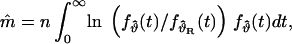
Evaluation of ĥ(x)
The parameters  and
and  were calculated by numerically evaluating the integrals in Eqs. 16a and 16b using the simple trapezoidal rule and exponentially increasing interval widths. Limited computer dynamic range was corrected for using the algorithm described in Appendix B.
RESULTS AND DISCUSSION
Distributions of log-likelihood ratios
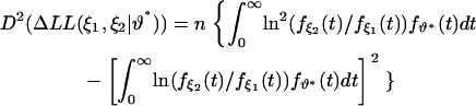
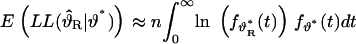
Ion channel gating models consist of a scheme, i.e., a number of closed and open states with a given connectivity among them, and a set of numeric parameters, i.e., the values of the transition rates (Fig. 1). Because of the underlying Markovian process the distributions of open and closed dwell times are mixtures of exponentials. As a usual first step in identifying a model, one is simply concerned about the probability density function (pdf) of either closed or open dwell times. In this context the model Ξ is described by the shape, i.e., the number of exponential components, of the pdf (which reflects the number of relevant single-channel states), and the parameter vector x, which consists of the set of time constants τ1, τ2, …τk and fractional amplitudes a1, a2, …ak−1. Usually, a particular number of exponential components is first assumed after visual inspection of the dwell-time histogram of interest, and then the parameter vector ξ found that maximizes the LL function, defined as follows. If a set of n dwell times t1, t2,…tn is observed and the data are fitted to a model with pdf f, then 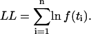 Note that the dwell times are measured in some unit of time (e.g., seconds or milliseconds); ti denotes here the dimensionless form of the dwell time, i.e., ti = (ith dwell-time)/(unit of time). Therefore, the pdf f of the variable ti is also dimensionless. In a typical situation the data are generated from a true (but unknown) model Θ described by parameter vector ϑ* (* will be used throughout this article to denote the true parameter vector which was used to generate the data); i.e., ti values are drawn from a distribution with pdf fϑ*. These data are then tentatively fitted to a model Ξ represented by the pdf fξ. This LL will be denoted LL(ξ|ϑ*) to emphasize that Θ (with parameter vector ϑ*) is the true model and Ξ (with parameter vector ξ) is the model assumed for fitting. LL(ξ|ϑ*) is itself a random variable, and the aim of the present work is to examine its distribution under various conditions relevant in practice. Without constraining generality, the focus will be on the closed-time distributions of the schemes shown in Fig. 1 (the parameters of the closed-time distribution are printed below each scheme).
FIGURE 1.

Gating schemes used for simulations. Rate constants are in s−1. Time constants (τcj, in milliseconds) and fractional amplitudes (acj) describe the closed-time distributions of the respective schemes. The schemes are organized in pairs. Both schemes in each row have identical open-time distributions; the closed-time distribution of each scheme in the right column (Scheme ΘR, for reduced) is a special case, under some constraint on the parameters, of the closed-time distribution of the scheme to its left (Scheme Θ). All reduced schemes are printed with parameter values corresponding to  (see text).
Distribution of ΔLL values obtained from describing the data by two alternative arbitrary schemes with fixed sets of parameters
This section lays the groundwork for addressing the full complexity of problems encountered in practice, by first solving a more simple situation. Thus, as a first step, assume that the data (generated from a true model Θ with vector ϑ*) are tentatively described by two arbitrary schemes Ξ1 and Ξ2 such that not only the shapes (numbers of components) of the pdfs are assumed, but also the parameter vectors ξ1 and ξ2 are fixed to any arbitrary values. The observed dwell times ti are distributed according to fϑ* and, if Θ contains only one gateway state (see all schemes in Fig. 1, except for Scheme 4), ti are also independent of each other. Thus, the random variables 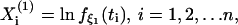 are also identically distributed and independent, and the same is true for the two series
 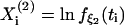 and
and 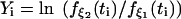 As
As 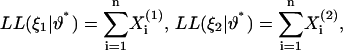 and
and 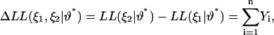 by the central limit theorem all three are asymptotically normally distributed, and the expectations and variances can be calculated as
 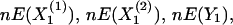 and
and 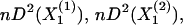 and nD2(Y1), respectively. Thus, for any model Ξ and any arbitrary fixed vector ξ,
 |
(1) |
 |
(2) |
while for any pair of models Ξ1, Ξ2 and arbitrary fixed vectors ξ1 and ξ2,
 |
(3) |
 |
(4) |
The validity of Eqs. 1–4 was confirmed using simulated data. E.g., 1000 independent events lists (see Materials and Methods), 500 closed events each, were simulated using Scheme 2 (Fig. 1). The LL for observing the closed-time distribution of each events list assuming either Scheme 2R or 2, with fixed parameters (in this case using the real parameters listed in Fig. 1), was evaluated for both cases. The histograms of the obtained LL (Fig. 2, A and B) and ΔLL (Fig. 2 C) values were well fit by Gaussian pdfs (solid lines) with mean and variance predicted by Eqs. 1 and 2 (Fig. 2, A and B) or Eqs. 3 and 4 (Fig. 2 C). Note that the distribution of ΔLL extends to the negative range (Fig. 2 C, light bars), although Ξ2 was chosen to be the true scheme Θ. This is because, even though ϑ* is the true parameter vector, the LL function is typically at a maximum at some different parameter vector (the ML estimate  ; see below). Therefore, the description by the correct distribution (Scheme 2) sometimes yields smaller LL-values than that using the incorrect (and even simpler) distribution (Scheme 2R).
FIGURE 2.

Distributions of LL and ΔLL values obtained from comparing two models with arbitrary fixed parameters. (A–C) One-thousand independent events lists, 500 closed events each, were simulated using Scheme 2. The LL of the observed closed-time distribution assuming either Scheme 2 or Scheme 2R, with rates printed in Fig. 1, was determined for each events list. These LL-values for assuming (A) Scheme 2R ( ) and (B) Scheme 2 (
 ), as well as (C) their differences (
 ), were binned to obtain the histograms shown. Light-colored bins in C identify cases in which ΔLL was negative. Solid fit lines are appropriately scaled (by the bin-width times the number of events lists) Gaussian pdfs with means and variances predicted by Eqs. 1 and 2 (A and B) or Eqs. 3 and 4 (C).
If t and  is time in two different units,
  and f and
  are the pdfs expressed using those two units, then
 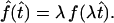 If LL and
  are obtained using these two time units, it is easy to show—using an integral transform on the variable t—that
 |
and
 |
Thus, the expectation of LL depends on the time unit, while its variance does not. In contrast, neither the expectation, nor the variance of ΔLL, depends on the time unit, as can be shown by an integral transform on the variable t in Eqs. 3 and 4 (for Eq. 3 this also follows from the latter two equations).
The integrals in Eqs. 1 and 2 can be performed numerically (see Appendix B), but also explicitly if fξ is single-exponential. If both fϑ* and fξ are single-exponential pdfs with time constants τϑ and τξ, respectively, then  and
and 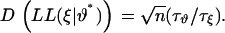 E.g., if
  and the data are fitted with the proper distribution, then
 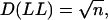 and E(LL) = −n · 3.303 if the pdf is expressed in units of ms−1 or E(LL) = n · 3.605 if the pdf is expressed in units of s−1 (see above, λ = 1000). If fξ is single-exponential but fϑ* is multiexponential, then Eqs. 1 and 2 can be written in the explicit form of
 |
and
 |
Representation of nested pairs of models
A simpler model is a submodel of a broader model if it can be identified with the broader model under some restriction on the parameters of the latter. The schemes in Fig. 1 are organized in such pairs. The schemes in the right column, with notation R (for reduced), can be identified with the schemes to their left under some particular restraint. The open-time distributions are identical for each pair of schemes, while the closed-time distributions of the schemes to the left are more complicated than those of the schemes to the right.
For instance, the closed-time distribution of Scheme 1 is defined by two free parameters, τc1 and τc2 (Fig. 3 A; for this particular closed-time distribution the fractional amplitudes ac1 and ac2 are functions of the two time constants τc1 and τc2). Scheme 1R is a special case of Scheme 1 in which, e.g., τc1 is fixed to zero. Thus, the parameter space of Scheme 1R (ΩR) is a one-dimensional line within the two-dimensional full parameter space Ω of Scheme 1 (Fig. 3 C, vertical shaded line). (Equivalently, in terms of rates, the closed-time distribution of Scheme 1 is defined by k12 and k23, and reduces to that of Scheme 1R, e.g., if k23→∞.)
FIGURE 3.

Asymptotic behavior of the ML estimate  when the correct scheme or its subset is assumed. (A,D) One-thousand independent events lists, 10,000 closed events each, were simulated using Schemes 1 and 2, and the closed-time distribution of each events list was ML-fitted to the generating scheme. Obtained parameter vector estimates
  are plotted as solid dots in two-dimensional space for Scheme 1 (A) and in three-dimensional space for Scheme 2 (D). The intersection of the solid auxiliary lines marks the location of the true parameter vector ϑ*. (B,E) Histograms of ML-estimates of τc obtained by fitting the same events lists with the respective reduced Schemes 1R and 2R (i.e., by single-exponential distributions). The histograms are centered on the mean closed times of Scheme 1 and 2; 1012.5 ms (B) and 46 ms (E). (C,F) Unconstrained (
 solid dots) and constrained (
 shaded x-marks, appear merged into shaded lines) parameter vector estimates plotted together in three-dimensional space for Scheme 1 (C) and in three-dimensional space for Scheme 2 (F). The vertical shaded line in C and the shaded line identified by the long arrow in F represent ΩR for those two cases. The slanting shaded line in A and C contains all parameter vectors that define distributions with a mean identical to that of Scheme 1 (1012.5 ms).
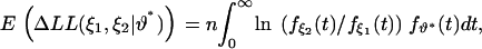
Analogously, the closed-time distribution of Scheme 2 contains three free parameters, τc1, τc2, and ac1 (Fig. 3 D). Scheme 2R is a special case of Scheme 2, e.g., under the constraints τc1 = τc2, and ac1 is any fixed value. Thus, the parameter space ΩR of Scheme 2R is a one-dimensional line (one free parameter) within the three-dimensional full parameter space Ω of Scheme 2 (Fig. 3 F, shaded line identified by arrow).
Distribution of Δll values obtained from fitting the data with the correct scheme and its subset, using the ML estimates of the parameters
In practice, the parameters of any fitted scheme Ξ are left free and optimized by ML; i.e., the particular vector  which maximizes the LL, is chosen. Fitting a submodel of Ξ to the data is identical to restricting the search for the best parameter vector to a subset ΩR of the full parameter space Ω. This ML estimate within ΩR will be denoted
Because the fitted parameter vectors are not fixed, the direct applicability of Eqs. 3 and 4 is limited. However, if the fitted model is the correct model Θ, and certain regularity criteria are met (Conditions I–VI in Appendix A), then the ML estimate  is asymptotically normally distributed around the true parameter ϑ*, and converges to ϑ* with probability 1 as n increases (29–31). Moreover, even if a set of incorrect restrictions is imposed on the true model, i.e., ϑ* ∉ ΩR, the restricted ML estimate
  converges in most cases to some particular point in ΩR. (For instance, if a set of data is fitted by a single-exponential pdf, the ML estimate of the time constant converges to the mean of the true distribution; see the note in Appendix A.) This best parameter within ΩR will be denoted ϑR*. (All reduced schemes in Fig. 1 are printed with parameter values corresponding to ϑR*.)
Fig. 3 provides a visual representation of these behaviors. One-thousand independent events lists, with 10,000 closed events each, were simulated using Schemes 1 and 2 (Fig. 1), and the closed-time distributions were fitted to the same schemes, and to the respective reduced schemes 1R and 2R, using ML. The solid dots in Fig. 3, A and D, show the unconstrained  estimates in two-dimensional space for Scheme 1 (Fig. 3 A) and in three-dimensional space for Scheme 2 (Fig. 3 D)—in both cases these estimates scatter closely around their true values marked by the intercept of solid auxiliary lines. Fig. 3, B and E, show histograms of τc estimates obtained from the restricted fits to the submodels 1R and 2R; both approximate narrow Gaussians centered on the respective mean closed times of 1012.5 ms (Fig. 3 B) and 46 ms (Fig. 3 E) predicted by the true generating schemes (Fig. 1). The corresponding
  vectors are shown in Fig. 3, C and F, as shaded X-marks.
Because for large n, the value of  becomes very similar to ϑ*, and
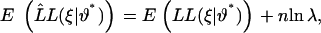
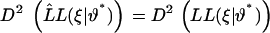
  to ϑR*, it might be expected that the distribution of LL values obtained from the free or restricted ML procedure will not be very different from that obtained when the fit parameters are fixed to ϑ* or ϑR*, respectively. Thus, if the data are generated using model Θ with true parameter vector ϑ*, ΩR is a closed subset of Ω such that ϑ* ∉ ΩR, and the data are ML-fitted with the correct model and its subset, then
 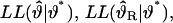 and
and  are all asymptotically normally distributed with means and variances approximated as follows. For the ML fit to the true model,
 |
(5) |
and
 |
(6) |
for the ML fit to the subset of the true model,
 |
(7) |
and
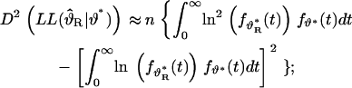 |
(8) |
and, finally, for the obtained log-likelihood ratio,
 |
(9) |
and
 |
(10) |
Appendix A provides a mathematically exact formulation of the above intuitive statements together with the proofs; Eqs. 5 and 6 are formulated as Statement 3, Eqs. 7 and 8 as Statement 4, and Eqs. 9 and 10 as Statement 5 (for an equation on a related problem, see (30)). Appendix B provides technical advice for numerically calculating the above integrals. The online Supplementary Material shows that the conditions required for the proof of Statement 3 are met by the multiexponential pdfs relevant to ion-channel dwell-time distributions. Note that neither Eq. 9 nor Eq. 10 depends on the time unit.
An important condition for Eqs. 9 and 10 to hold (Statement 5, Appendix A) is ϑ* ∉ ΩR, which implies that ϑ* and ϑR* are two distinct points of the full parameter space Ω. (The opposite case, ϑ* ∈ ΩR, means the restricted model is the correct model and ϑR* = ϑ*.) This condition is illustrated in Fig. 3, C and F, which replots, in the same panel, free  estimates (solid dots) and
  estimates (shaded x-marks) for Scheme 1 (Fig. 3 C) and Scheme 2 (Fig. 3 F). Note the clear separation of the sets of solid and shaded symbols in parameter space.
Extensive simulations were done to verify the validity of Eqs. 9 and 10 (Statement 5), as well as to test how fast the distributions of 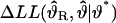 converge to their predicted shapes. Fig. 4 illustrates a subset of the results, for Scheme 1 versus 1R (Fig. 4 A), 2 versus 2R (Fig. 4 B), and 4 versus 4R (Fig. 4 C), with n ranging from 125 to 10,000; it affords the following conclusions.
FIGURE 4.

Distributions of free ΔLL values for the case when the broader scheme is true. (A–C) For each of Schemes 1, 2, and 4, events lists of increasing lengths, ranging from 125 to 10,000 closed events, were simulated, with 1000 independent events lists for each scheme and each length. The closed-time distribution of each events list was fitted by ML to both the appropriate generating scheme and its reduced pair. The resulting ΔLL values for Scheme 1 versus 1R (A), Scheme 2 versus 2R (B), and Scheme 4 versus 4R (C), are plotted in the form of histograms. The solid lines are appropriately scaled Gaussian pdfs with mean and variance predicted by Eqs. 9 and 10.
First, the description of the distributions of ΔLL is excellent for all three models when n ≥ 2000, but already reasonably good for ∼250 events. Naturally, no negative ΔLL values occur when nested models are compared using the ML estimates of the parameters, unlike for the case shown in Fig. 2 C, where ΔLL was obtained from comparison of fixed-parameter schemes. This is because ϑR* is also a member of the full parameter space Ω. Therefore, in the cases when LL happens to exceed LL(ϑ*|ϑ*), the unconstrained ML procedure will find a LL maximum corresponding to a
  (instead of
  as assumed for Eqs. 9 and 10), and ΔLL will never be negative. Thus, the ΔLL distribution is truncated at zero, and the discrepancy between the histograms and predicted lines in Fig. 4 (normal distributions characterized by Eqs. 9 and 10) can be ascribed to the data corresponding to the missing negative tail, spread over the positive part of the distribution. The fit improves as n increases and the lower tail of the Gaussian diverges away from zero (as predicted by Eqs. 9 and 10). Note that the distinction between all three pairs of closed-time distributions in Fig. 4 is relatively difficult; for easier cases the convergence of the distribution of ΔLL to the predicted Gaussian pdf will be faster.
Second, although Schemes 2 and 4 predict identical closed-time distributions (Fig. 1), Scheme 4 has two gateway states. Therefore, for Scheme 4 the durations of adjacent closed events are correlated (long closed events, transitions to state C1, are clustered, as are the shorter closed events generated by state C2), hence the independence of t1, t2, …tn, necessary for the proofs of asymptotically normal behavior and for Eqs. 2, 4, 6, 8, and 10, does not hold. Nevertheless, the simulations clearly show that the Gaussian prediction, together with the above equations, provides identically good descriptions of the distributions of LL (not shown) and ΔLL values for Scheme 4 (Fig. 4 C) as for Scheme 2 (Fig. 4 B). This need not be surprising, as ΔLL depends only on the distribution, not on the sequence, of observed closed durations, and the distributions are predicted to be identical for both schemes beyond a few tens of events.
Distribution of ΔLL values obtained from fitting the data with the correct scheme and its generalization, using the ML estimates of the parameters—the case of one extra parameter
The case that, between a more complicated scheme and its subset, the restricted model is the correct one, has long been studied (29–31). If a set of regularity criteria (Conditions I–VI in Appendix A) are met, 2ΔLL is asymptotically  distributed with a degree of freedom (k) equal to the difference in the number of free parameters between the two compared models (the χ2-theorem). However, it has not yet been examined whether the required regularity criteria are satisfied in models that describe ion-channel gating. This and the following section examine this question for two cases; the case of one extra parameter (k = 1), and the more common case of one extra exponential component (two extra parameters, k = 2), in the more complicated scheme.
The pair of Schemes 1 and 1R exemplifies the situation for one extra parameter; the closed-time distribution of Scheme 1 is defined by two (τc1 and τc2), that of Scheme 1R by one free parameter (τc). The full parameter space Ω is the subset of two-dimensional space bounded by τc1 ≥ 0 and τc2 ≥ τc1; the reduced space ΩR is the line τc1 = 0 (Fig. 5 A). When Scheme 1R is true, ϑ* ∈ ΩR. Thus, ϑ* lies on the boundary of Ω, while the χ2-theorem requires Conditions I–VI to hold in an open region in Ω which contains ϑ*. Although less well known, the distribution of 2ΔLL has been studied for several specific geometries of Ω and ΩR in which ϑ* is either a boundary point of ΩR (but an interior point of Ω; e.g., (40–43)), or, like here, a boundary point of Ω itself (44). However, the mathematical treatment of these situations still required in each case fulfillment of the regularity criteria on the boundary itself. Unfortunately, these criteria do not apply in the present situation for τc1 = 0. E.g., contrary to Condition V (Appendix A), the information matrix I(ϑ) is infinite there (see Supplementary Material, Section 2).
FIGURE 5.

Asymptotic behavior of the ML estimate  when the correct scheme or its generalization is assumed—the case of one extra parameter. (A) One-thousand independent events lists, 10,000 closed events each, were simulated using Scheme 1R, and the closed-time distribution of each events list was ML-fitted to the more general Scheme 1. Obtained parameter vector estimates
  are plotted as solid dots in full (two-dimensional) parameter space Ω. The vertical shaded line represents ΩR (i.e., τc1 = 0); the intersection of this line with the horizontal solid line marks the location of the true parameter vector ϑ*. (B) Histogram of ML-estimates of τc obtained by fitting the same events lists with the true generating Scheme 1R (i.e., with a single-exponential distribution). The histogram is centered on the true parameter τc = 1012.5 ms. (C) Unconstrained (
 solid dots) and constrained (
 shaded x-marks, appear merged into a shaded line) parameter vector estimates plotted together in full, two-dimensional, parameter space Ω.
To test whether this fact compromises any of the properties of the ML procedure, extensive simulations were done using Scheme 1R, followed by ML fits to the closed-time distributions of both Schemes 1R and 1. Fig. 5 shows the scatter of the parameter estimates for 1000 independent simulated events lists (10,000 closed events each). Although ϑ* lies on the boundary of Ω, the unconstrained ML estimates  (Fig. 5 A, solid dots) are still approximately normally distributed on the half-plane. The restrained ML estimate
  is, of course, approximately normally distributed on the line (histogram in Fig. 5 B). As
  the sets of
  and
and  are merged in Ω space (solid dots and shaded x-marks, Fig. 5 C; compare to Fig. 3 C), and Eqs. 9 and 10 do not apply (see Statement 5, Appendix A).
Next, the distributions of  were examined. If 2ΔLL were distributed as
  then, equivalently, ΔLL should follow a Γ-distribution with shape parameter k/2 and scale parameter 1 (Γ(k/2, 1). Thus, if theχ2-theorem holds, the pdf of the distribution of ΔLL values should be given by
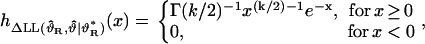 |
(11) |
where  Fig. 6 A shows histograms of ΔLL
 obtained from events lists with increasing n, simulated using Scheme 1R. In contrast to the case in which the broader scheme is true (Fig. 4 A), the distribution of ΔLL does not shift with increasing n; instead, it is well fit, already for as few as 125 events, by a Γ(k/2, 1) distribution with k = 1 (solid line; compare to k = 2, thin line). To better resolve the distribution at small x, the natural logarithm of ΔLL, lnΔLL, was also binned to construct histograms (Fig. 6 B). This transformation converts the Γ(k/2, 1) pdf into a new pdf,
 |
(12) |
a function that peaks at z = ln(k/2). (The same transformation is routinely used for the display of multiexponential distributions of ion-channel dwell-times (4).) After this transformation, the lnΔLL distributions were still well fit with parameter k = 1 (Fig. 6 B, solid lines; compare to k = 2, thin lines). Finally, when the ΔLL values themselves were ML-fitted to the pdf in Eq. 11, with k as a free parameter, these fits returned k ≈ 1 in each case (not shown). Thus, although ϑ* lies on the boundary of Ω, the ML estimates
  and
and  are still asymptotically normally (or half-normally) distributed, and ΔLL is asymptotically distributed as Γ(1/2, 1); i.e., 2ΔLL approaches
FIGURE 6.

Distribution of free ΔLL values when the restricted scheme is true—the case of one extra parameter. (A,B) Events lists with numbers of closed events ranging from 125 to 10,000, with 1000 independent events lists each, were simulated using Scheme 1R. The closed-time distributions were ML-fitted to both Schemes 1R and 1. Obtained  (A) and
  values (B) were binned to construct histograms. The solid lines in A and B are plots of Eqs. 11 and 12, respectively, using k = 1. As a comparison, thin lines illustrate the case of k = 2.
Distribution of ΔLL values obtained from fitting the data with the correct scheme and its generalization, using the ML estimates of the parameters—the case of one extra exponential component
A far more common problem in practice is whether a fit to a dwell-time distribution is significantly improved by allowing one extra exponential component (9,21–23,26,32,45–51). The broader model in this case contains two extra free parameters (a time constant and a fractional amplitude), i.e., the full parameter space Ω has two more dimensions than ΩR. Fig. 7 illustrates Ω for the closed-time distribution of Scheme 2; the subset of two-dimensional space bounded by τc1 ≥ 0, τc2 ≥ τc1, ac1 ≥ 0, and ac1 ≦ 1. The term ΩR, which describes Scheme 2R, is a one-dimensional line in Ω (see Fig. 3 F), defined, e.g., by the constraints τc2 = τc1, and ac1 = fixed to any value. Thus, once again, ΩR lies on the boundary of Ω.
However, a more important problem also arises in this case. This is that once τc2 = τc1, the value of ac1 is immaterial—the dwell-time distributions are identical for any ac1. The same problem arises for the other two ways in which Ω can be reduced to ΩR (if ac1 = 1, τc2 is immaterial, if ac1 = 0, τc1 is immaterial). Thus, all points of Ω that lie on a jointed line like the one drawn in Fig. 7 (solid line) represent identical distributions. This is a serious violation of the regularity criteria which assume that different parameters ϑ correspond to different distributions (Condition I, see Appendix A). 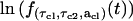 is constant on any line segment defined by τc2 = τc1 (fixed), 0 ≤ acl ≤ 1 (Fig. 7, vertical segment of solid line); therefore
  on the whole plane τc2 = τc1. Consequently, the information matrix I(ϑ) is singular for all ϑ ∈ ΩR (also if ΩR is defined as ac1 = 0 or ac1 = 1, see Supplementary Material, Section 3), rather than positive definite as required by Condition V.
Given the above irregularities, the properties of the ML procedure were extensively tested on events lists simulated using Scheme 2R and fitted to the closed-time distributions of both Schemes 2R and 2. Because  is expected to scatter in a broad region of Ω, special care had to be taken to identify it (see Materials and Methods). As expected, the unconstrained
  estimates were scattered in the region of Ω surrounding the jointed line, which contains the points that all represent Scheme 2R (Fig. 8 A, solid dots), while the constrained ML estimates were approximately normally distributed on the line around the true parameter τc (histogram in Fig. 8 B). Once again, as ϑ* ∈ ΩR, the sets of
  and
and  are merged in Ω space (Fig. 8 C, shaded x-marks identified by shaded box, and solid dots; compare to Fig. 3 F), and Eqs. 9 and 10 do not apply (see Statement 5, Appendix A).
FIGURE 8.

Asymptotic behavior of the ML estimate  when the correct scheme or its generalization is assumed—the case of one extra exponential component. (A) One-thousand independent events lists, 10,000 closed events each, were simulated using Scheme 2R, and the closed-time distribution of each events list was ML-fitted to the more general Scheme 2 (see Materials and Methods for details). Obtained parameter vector estimates
  are plotted as solid dots in three-dimensional parameter space Ω. (B) Histogram of ML-estimates of τc obtained by fitting the same events lists with the true generating Scheme 2R (i.e., with a single-exponential distribution). The histogram is centered on the true parameter τc = 46 ms. (C) Unconstrained (
 solid dots) and constrained (
 shaded x-marks, identified by shaded box) parameter vector estimates plotted together in full, three-dimensional, parameter space Ω. The subset ΩR (shaded line identified by upper arrow) is arbitrarily drawn as the line defined by τc1 = τc2, ac1 = 0.5.
To study the distributions of  for this situation, the obtained
  were binned to form histograms (Fig. 9). Interestingly, these histograms were not well fit by the pdfs of Γ(k/2, 1) distributions, whether k = 1 or k = 2 was assumed (Fig. 9 A, thin lines; compare to Fig. 6 A). In particular, a large fraction of all ΔLL values fell into the first bin. A similar deviation of 2ΔLL from a χ2 statistics was observed in a study using ML for fitting macroscopic ionic currents (52), and was attributed to the constraint that rate constants are nonnegative. However, as the χ2-theorem clearly applies for the comparison of Schemes 1 versus 1R (Fig. 6), a more likely reason for the unexpected behavior of
  (Fig. 9) is the fact that Scheme 2R cannot be identified with a unique point in the parameter space of Scheme 2 (Fig. 7).
FIGURE 9.

Distribution of free ΔLL values when the restricted scheme is true—the case of one extra exponential component. (A,B) Events lists with numbers of closed events ranging from 125 to 10,000, with 1000 independent events lists each, were simulated using Scheme 2R. The closed-time distributions were ML-fitted to both Schemes 2R and 2. Obtained  (A) and
  values (B) were binned to construct histograms. Thin lines in A and B are plots of Eqs. 11 and 12, respectively, using k = 1 and k = 2 (see Fig. 6); solid lines are plots of Eq. 14 in A, and of its appropriate transform in B.
To obtain a better resolution in the small-ΔLL range, histograms were again constructed from the natural logarithm of ΔLL (Fig. 9 B, thin lines show appropriately transformed Γ(k/2, 1) pdfs with k = 1 and k = 2; see Fig. 6 B). This representation clearly shows that the ΔLL values belong to a mixture of two distinct distributions, one of which is clustered around machine-zero (the smallest positive number a computer algorithm can return) with a pdf approximating a δ-function. The fractional amplitude of this component decreases as n increases (Fig. 9 B). (The parallel apparent shift to the right of the δ-function is an artifact due to the decreasing floating-point precision to which ΔLL values are calculated, since ΔLL is obtained as the difference of two LL values which themselves increase linearly with n.)
To provide an empirical description of the two components of these distributions, an arbitrary cutoff value of ΔLL ≥ 10−6 was set (ln (ΔLL) = −13.8). The values of ΔLL < 10−6 were assumed to belong to the component characterized by the δ-function, whereas the values of ΔLL ≥ 10−6 were separately considered.
Fig. 10 A shows the fractional amplitude (α) of the latter component as a function of n, determined from an extensive series of experiments including the ones illustrated in Fig. 9. The solid line in Fig. 10 A is a least-squares fit to the observed α(n) of the empirical function
 |
(13a) |
with best fit parameters A1 = 149.2 and A2 = 2.927 (log, 10-base logarithm).
FIGURE 10.

Parameters of the empirical distribution which best fits ΔLL—the case of one extra exponential component. Events lists with numbers of closed events (n) ranging from 125 to 10,000, 1000 independent events lists each, were simulated using Scheme 2R. The closed-time distributions were ML-fitted to both Schemes 2R and 2. (A) Fraction (α) of  values
  plotted as a function of n (solid circles) and the fit line described by Eq. 13a (solid line). (B) The set of
  was fitted by ML to a pdf of the form (1–β)h1 + βh2, with β as a free parameter, where h1 and h2 are Γ(k/2, 1) pdfs (Eq. 11) with k = 1 and k = 2, respectively. Solid circles and error bars show estimates of β and 0.5-unit likelihood intervals. The solid line is a fit of the solid circles by Eq. 13b. Shaded triangles in A and B illustrate the results of an identical analysis for a set of 1000 independent events lists simulated using Scheme 3R and fitted to both Schemes 3R and 3 (see Fig. 11).
The above results recall studies in which 2ΔLL was shown to be a mixture of  (a component identically zero),
  and
and  for cases in which ϑ*R is on the boundary of ΩR or Ω but the regularity criteria are satisfied (40–44). Therefore, as ΔLL
 values greater than 10−6 were still not well fit by either a Γ(1/2, 1) or a Γ(2/2, 1) distribution, it seemed natural to fit all ΔLL ≥ 10−6 to a mixture of the above two distributions—with the fractional amplitude β of the latter component left as a free parameter (0 ≤ β ≤ 1). Such a pdf indeed improved the quality of the fit significantly, as compared to fitting with just one or the other component. Interestingly, the β-values returned by these ML-fits were also not constant, but increased with increasing n, from β ≈ 0.6 (for n = 125) to β ≈ 0.9 (for n = 10,000; Fig. 10 B, solid dots). The solid line in Fig. 10 B is a least-squares fit to the obtained β(n) of the empirical function
 |
(13b) |
with best-fit parameters B1 = 212.2 and B2 = 2.703.
Thus, the empirical pdf of ΔLL can be assembled as
 |
(14) |
where α(n) = 1–149.2/(2.927 + log n)4, and β(n) = 1–212.2/(2.703 + log n)4. (δ0(x) is a δ-function centered on zero.) The solid lines in all panels of Fig. 9, A and B, illustrate the pdf predicted by Eq. 14 (transformed as in Eq. 12 for the panels in Fig. 9 B).
However, β(n) from Eq. 13b did not provide a uniformly good description for the whole range of ΔLL ≥ 10−6. When the ML fits to Eq. 14, with β as a free parameter, were repeated for ΔLL ≥ 0.3, the β-values converged to β = 1 in each case. Because in most statistical applications, in particular in log-likelihood ratio tests, a good prediction of the tail of the distribution is most important, a practically useful empirical description of the pdf of  is given by Eq. 14 with α(n) from Eq. 13a and β = 1. In this context, for x > 0, Eq. 14 simplifies to
 |
(15) |
How representative is the case of one versus two exponential components of the general case of one extra exponential component? The regularity violations (Fig. 7) apply identically for all those cases. But, most importantly, does Eq. 14 (or 15) provide a good description of the distribution of ΔLL for every such case? To address this question, 1000 independent events lists (1000 closed events each) were simulated using Scheme 3R, and the closed-time distributions were ML-fitted to both Schemes 3R and 3, i.e., to pdfs with four and five exponential components. The distribution of obtained
 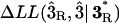 values is displayed in Fig. 11 in the form of a linear (Fig. 11 A) and a logarithmic (Fig. 11 B) histogram. This distribution is remarkably similar to the one obtained from the comparison of Schemes 2R and 2, 1000 events (Fig. 9 A, B, row 4). In particular, it was not well fit by Γ(k/2, 1) pdfs whether k = 1 or k = 2 was used (Fig. 11, A and B, thin lines), but was well fit by the pdf described in Eq. 14 (Fig. 11, A and B, solid line). Both the fraction of ΔLL greater than 10−6 (Fig. 10 A, shaded triangle), and the best β-value for ΔLL ≥ 10−6 (Fig. 10 B, shaded triangle) were closely similar to those obtained for one versus two exponential components. Also, when only the tail of the distribution (ΔLL ≥ 0.3) was fitted, the fit again converged to β = 1. Thus, the results illustrated in Figs. 9–11, as well as Eq. 14 or 15, characterize the distribution of
 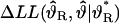 for the general case of one extra exponential component.
FIGURE 11.

Distribution of free ΔLL values when the restricted scheme is true—the case of five versus four exponential components. (A,B) One-thousand independent events lists, 1000 closed events each, were simulated using Scheme 3R. The closed-time distributions were ML-fitted to both Schemes 3R and 3. Obtained  (A) and
 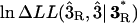 values (B) were binned to construct histograms. Thin lines in A and B are plots of Eq. 11 and Eq. 12, respectively, using k = 1 and k = 2; the solid line is a plot of Eq. 14 in A, and of its appropriate transform in B.
Strategies for model discrimination
Log-likelihood ratio test (LLR-test)
The log-likelihood ratio test (LLR test) is used to evaluate whether a model Θ or its submodel ΘR is more appropriate to describe the data. If ΘR is true (the null hypothesis) and the regularity criteria are satisfied 2ΔLL is asymptotically  -distributed (k is the difference in the number of free parameters (28,29)), and the chance of occurrence of a ΔLL greater than or equal to that observed is given by the integral of the tail of the
  pdf between 2ΔLLobserved and infinity. The submodel ΘR is rejected (Θ is accepted) at significance level P (typically P = 0.10, 0.05, or 0.01) if 2ΔLLobserved is larger than the
  -value corresponding to P.
The LLR test has been used in the past for comparison of nested pairs of ion-channel gating models (e.g., (2,32,53)), but without verifying the validity of the required regularity criteria. As pointed out in the previous two sections, these criteria apply in the interior of Ω, but not at its boundary. Thus, a  distribution for 2ΔLL under the null hypothesis is guaranteed only if ΘR is an interior point of Θ, e.g., when the restricted model consists of fixing a subset of the parameters or introducing linear constraints or microscopic reversibility (6). Interestingly, 2ΔLL was found
  -distributed also for introduction of one superfluous parameter (Fig. 6) even if
  was a boundary point of Θ but distinct points
  corresponded to distinct pdfs (see Fig. 5).
However, for the most frequent application of judging the improvement of the fit of a dwell-time distribution by a multiexponential pdf upon introduction of one extra exponential component (e.g., (9,16,22,23,32,45–51)), the assumption that 2ΔLL is  -distributed under the null hypothesis is unwarranted and wrong (Fig. 9). A practically useful empirical pdf of ΔLL for that case is given by Eq. 15. The area under the tail of this pdf can be calculated; the cutoff value for ΔLL for a fixed P-value and n is ΔLLcutoff = ln(α(n)/P). Table 1 lists a set of such calculated ΔLLcutoff values for n ranging from 125 to 100,000, and for P = 0.10, 0.05, and 0.01. Thus, using Table 1, a valid LLR test can now be used for discriminating whether l or l+1 exponential components are present in a dwell-time distribution (corresponding to l vs. l+1 single-channel states in a gating model). Fig. 12 illustrates Type I errors obtained using the LLR test based on Table 1, and P-values of 0.10 (circles), 0.05 (squares), and 0.01 (triangles), for a large set of data simulated using Scheme 2R and fitted by Schemes 2R and 2 (Fig. 1). These errors scatter closely around their predicted values (horizontal lines). It must be noted that, although the overall distribution of 2ΔLL differs substantially from a
  for all but extremely large n, the tail of the distribution does not (note the weak dependence on n of ΔLLcutoff in Table 1; see also Fig. 9). Thus, fortunately, conclusions drawn in previous studies based on the unwarranted
  -assumption are unlikely to be far wrong.
TABLE 1.
ΔLL cutoff values for the LLR test to distinguish l vs. l+1 exponential components
| Number of events | P < 0.10 | P < 0.05 | P < 0.01 |
|---|---|---|---|
| 125 | 2.0359 | 2.7290 | 4.3385 |
| 250 | 2.0974 | 2.7906 | 4.4000 |
| 500 | 2.1414 | 2.8346 | 4.4440 |
| 750 | 2.1615 | 2.8546 | 4.4641 |
| 1000 | 2.1738 | 2.8669 | 4.4764 |
| 1250 | 2.1824 | 2.8755 | 4.4850 |
| 1500 | 2.1889 | 2.8820 | 4.4915 |
| 1750 | 2.1940 | 2.8871 | 4.4966 |
| 2000 | 2.1982 | 2.8914 | 4.5008 |
| 5000 | 2.2221 | 2.9152 | 4.5246 |
| 10,000 | 2.2356 | 2.9288 | 4.5382 |
| 20,000 | 2.2464 | 2.9395 | 4.5490 |
| 100,000 | 2.2641 | 2.9572 | 4.5667 |
| ⋮ | |||
| Infinite | 2.3026 | 2.9957 | 4.6052 |
FIGURE 12.

Type I errors obtained using the LLR test based on Table 1. Events lists with numbers of closed events ranging from 125 to 10,000, one-thousand independent events lists each, were simulated using Scheme 2R and the closed-time distributions ML-fitted to both Schemes 2R and 2. Circles, squares, and triangles show the fraction of cases in which the obtained ΔLL was larger than the cutoff specified in Table 1 for P-values of 0.10, 0.05, and 0.01, respectively. Horizontal lines indicate the expected values.
Akaike information criterion (AIC) and Schwarz criterion (SC)
The goodness of fit by any two alternative models, whether nested or not, is frequently compared using the Akaike information criterion (AIC, (33)) or the Schwarz criterion (SC, (34)). Although the SC was originally tested on LL estimates obtained from fitting the entire sequence of single-channel closed and open durations (7), it can be adapted to ML fits of a dwell-time distribution for gating schemes with only one gateway state (21). In the present context, a larger model is considered better by the AIC if ΔLL > k, or by the SC if ΔLL > 0.5kln(2n), where k is the difference in the number of free parameters, and n is the number of fitted, closed or open, events. Both methods penalize more free parameters, but the SC also considers the size of the data set. The AIC (7,12,13,53–57) and the SC (7,12,21,26,57) have been widely used in ion-channel model discrimination. Their relative merit is debatable, as different studies found the SC either more (7), similarly (57), or even less (12) efficient than the AIC in identifying the right model.
New nonbiased decision strategy based on the parameter estimates and the distributions of ΔLL
For the comparison of a pair of nested models the LLR test exploits the knowledge of the distribution of ΔLL under the null hypothesis, but it does not take into account the distribution of ΔLL for the alternative case. The philosophy of the LLR test is to always accept ΘR unless the latter can be excluded with very high certainty. Thus, it is biased toward ΘR by ensuring that the Type I error (rejection of ΘR, although true) is kept at a constant (low) value, without trying to minimize the Type II error (rejection of Θ, although true). Although rewarding parsimony does have its merits (Occam's razor), identification of complexities using the LLR test will be inefficient for all but large amounts of data. An alternative philosophy, without an a priori bias, would be to always choose the model which seems more likely, i.e., to equalize the probabilities of the two types of error. Although this cannot be rigorously achieved, this section describes a new, semiempirical strategy attempting to approximate that aim. The decision is based on consideration of two aspects of the fit.
First, the fit parameter  itself is inspected. When ΘR is true, fitting with Θ in many cases yields parameters which are unreasonable. E.g., when a dwell-time distribution is ML-fitted with too many components, frequently the fit returns τi ≈ τj for i ≠ j, or ai ≈ 0 (Figs. 5 A and 8 A). For many, but not all, such cases ΔLL ≈ 0. Such fits (called overparameterized) are excluded from further analysis, i.e., ΘR is accepted as the better model. In practice, the following, somewhat arbitrary, set of criteria was adopted. A fit was defined as overparameterized, if either of the following three conditions applied:
For some i ≠ j 9/10 ≤ τi/τj ≤ 10/9.
For any i |ai| < 0.005.
ΔLL ≤ 0.0015n, where n is the number of dwell-times analyzed.
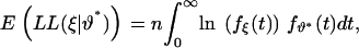
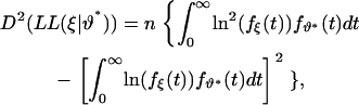
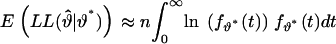
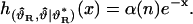
Second, if a fit returns a  which itself seems reasonable, the predicted pdfs of ΔLL are compared for the two possible situations, which are that either Θ or ΘR is true (Fig. 13). If ΘR is true,
 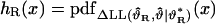 is given either by Eq. 11 (if the χ2-theorem holds; e.g., if ϑ*R is in the interior of Θ, or for a comparison involving one extra parameter such as that between Scheme 1 and 1R) or by Eq. 15 (for a comparison involving one extra exponential component such as that of Scheme 2 with 2R or 3 with 3R). If Θ is true, h(x) = pdf
  (x) is approximated by
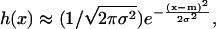 |
where m and σ2 are given by Eqs. 9 and 10, respectively. Fig. 13 allows visual comparison of appropriately scaled experimental histograms of hR(x) for the former case (hatched bars; obtained from fitting both Schemes 1R and 1 to events lists simulated using Scheme 1R), and of the corresponding h(x) (shaded bars; from fitting both Schemes 1R and 1 to simulated Scheme-1 events lists). Solid lines illustrate the theoretical pdfs predicted by Eq. 11 and Eqs. 9 and 10, respectively.
FIGURE 13.

Direct comparison of pdfs of ΔLL distributions for the cases in which the submodel or the full model is true. ΔLL values binned to construct the two histograms were obtained by ML-fitting both Schemes 1R and 1 to 1000 independent events lists (500 closed events each), simulated either using Scheme 1R (hatched bars) or using Scheme 1 (shaded bars). Binwidths were 0.1 and 0.5, respectively; and both histograms were normalized by dividing them by 1000 · binwidth to obtain histograms that integrate to unity. Solid lines plot the theoretical pdfs hR(x) and h(x) (Eqs. 11, 9, and 10, respectively). Flow chart (inset) summarizes the new decision algorithm.
Unfortunately, h(x) depends on ϑ* and ϑ*R (Eqs. 9 and 10) which are not known. To approximate h(x), the ML estimates  and
and  are substituted in place of ϑ* and ϑ*R. Thus, ĥ(x) is defined as
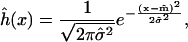 |
(16) |
where
 |
(16a) |
and
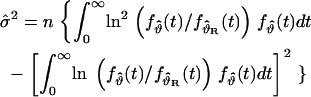 |
(16b) |
The model ΘR or Θ is then selected based on whether hR(x) or ĥ(x) is larger for x = ΔLLobserved.
Thus, the new strategy can be summarized as follows (Fig. 13, inset). The broader model Θ is accepted as the better model if
 is not overparameterized based on criteria 1–3, above.
For all other cases, the reduced model ΘR is preferred.
Performance of various decision strategies for the case of one extra parameter or one extra exponential component
The performances of the LLR test, the AIC, the SC, and of the new strategy described in the previous section, were compared on large sets of simulated data. Both the case of one extra parameter (Scheme 1 versus 1R) and that of one extra exponential component (Scheme 2 versus 2R) in the broader model was examined. For both cases, events lists of various lengths were simulated using either the respective Scheme ΘR or the respective Scheme Θ, 1000 independent events lists each. The closed-time distribution of each events list was ML-fitted to both schemes to produce  and ΔLL values. Finally, a decision was made for each events list using all four strategies described above. The results are summarized in Fig. 14 A for Scheme 1 versus 1R, and in Fig. 14 B for Scheme 2 versus 2R. The panels plot, for each set of 1000 events lists, the fraction of cases in which a given strategy (the LLR test is shown for P = 0.05) opted for the broader Scheme Θ. Events lists simulated using Scheme Θ are denoted by solid symbols, and those simulated using Scheme ΘR, by open symbols.
FIGURE 14.

Performance of various decision strategies in identifying the correct model. The cases of (A) one extra parameter (Scheme 1 versus 1R), and of (B) one extra exponential component (Scheme 2 versus 2R) in the broader model are illustrated. (A,B) Events lists with numbers of closed events ranging from 125 to 10,000, one-thousand independent events lists each, were simulated using either the full model Θ (Scheme 1 in A, Scheme 2 in B) or its submodel ΘR (Scheme 1R in A, Scheme 2R in B). For each events list the closed-time distribution was ML-fitted to both ΘR and Θ to produce fit parameters and ΔLL values. A decision in favor of either ΘR or Θ was then made using four different strategies. Symbols plot, for a given set of 1000 events lists, the fraction of cases in which a given strategy opted for Θ. Solid symbols denote events lists simulated using Θ, open symbols denote those simulated using ΘR. LLR test for P = 0.05, diamonds; AIC, triangles; SC, squares; new strategy, circles. Dotted lines illustrate symmetrical Type I and Type II errors expected for using the respective ideal ΔLLcut (see Fig. 15).
For Scheme 1 versus 1R hR(x) (Eq. 11) does not depend on n. Therefore, any strategy that uses a fixed cutoff is expected to give a constant Type I error irrespective of n. Accordingly, both the LLR test (which uses a constant ΔLLcutoff = 1.9207 for P = 0.05) and the AIC (which uses a constant ΔLLcutoff = 1) misclassified a constant fraction, ∼5% and ∼13%, respectively, of all Scheme-1R events lists (Fig. 14 A, open diamonds and triangles). For Scheme 2 versus 2R hR(x) (approximated by Eq. 15) shifts to the right with increasing n. Because the AIC uses a fixed cutoff (of 2 in this case; Fig. 15, C and D, long-dash line), the Type I error produced by the AIC increases slightly, from ∼10% at 125 events to ∼17% at 10,000 events (Fig. 14 B, open triangles; unlike in Fig. 14 A). Accordingly, the LLR test (P = 0.05) was performed in this case using Table 1, not a fixed cutoff value (Fig. 15, C and D, solid line). As a consequence, the Type I errors remain constant at ∼5% (Fig. 14 B, open diamonds), as expected for this type of test.
FIGURE 15.

Comparison of ΔLL distributions with cutoff values used by various strategies for evaluation of a pair of nested models. The cases of (A,B) one extra parameter (Scheme 1 versus 1R), and of (C,D) one extra exponential component (Scheme 2 versus 2R) in the broader model are illustrated. The value of ΔLL is plotted as a function of the number of closed events (n) using linear axes in A and C, and double-logarithmic axes in B and D. Lower shaded lines and shaded areas plot the expectations and mean ± SD ranges of the pdfs hR(x) (mean = 0.5, SD = 2−1/2 (Eq. 11) in A and B; mean = α(n), 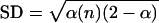 (Eq. 15) in C and D). Open shaded circles and error bars show observed averages and SD of ΔLL for sets of 1000 independent events lists simulated using the submodels ΘR (Scheme 1R in A and B; 2R in C and D) and ML-fitted with both ΘR and the respective Θ (Scheme 1 in A and B; Scheme 2 in C and D). Upper shaded lines and shaded areas plot the expectations and mean ± SD ranges of the pdfs h(x); i.e., Gaussian pdfs truncated at zero, with m and σ2 from Eqs. 9 and 10 for the scheme-pairs 1R/1 (A and B) and 2R/2 (C and D), respectively. Shaded circles and error bars show observed averages and SD of ΔLL for sets of 1000 independent events lists simulated using the full schemes Θ (Scheme 1 in A and B; Scheme 2 in C and D), and ML-fitted with both the respective ΘR and Θ. Black lines in A–D plot cutoff values used by the LLR test (P = 0.05, solid line), the AIC (long-dash line), and the SC (short-dash line). Dotted lines in A–D illustrate the respective ideal ΔLLcut values satisfying the equation
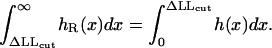
On the other hand, for small n, both methods produced large Type II errors, i.e., failed to recognize Scheme-Θ events lists as such (solid diamonds and triangles). E.g., only ∼33% of Scheme-1 events lists were correctly identified by the LLR test at P = 0.05 when 250 closed events were fitted, and only ∼16% when 125 closed events were fitted.
The SC proved to be extremely conservative in both cases (Fig. 14, A and B; squares). It produced negligible Type I errors (open squares, <2% in Fig. 14 A, <0.5% in Fig. 14 B), but was extremely inefficient in correctly identifying Scheme-1 events lists for all but very large n (Fig. 14 A, solid squares); and recognition of Scheme 2 was even less efficient (Fig. 14 B; solid squares).
As expected, the new strategy yielded the most symmetrical results (Fig. 14, A and B; circles). Two advantages of this approach over other tests should be noted. First, at low event numbers the decrease in Type II error, produced by the new strategy relative to the other three tests, is much larger than the increase in Type I error, resulting in a larger overall power of discrimination (Fig. 14, A and B). E.g., the new strategy identifies 72% of true Scheme-1 events lists already from 125 closed events (Fig. 14 A, solid circles), an improvement by 56% relative to the LLR test, at a cost of misclassifying 32% of Scheme-1R events lists of identical length (Fig. 14 A, open circles), a relapse of 27% relative to the LLR test. Second, at high event numbers the Type I error for the new strategy converges to zero (Fig. 14, A and B, open circles), unlike that for the LLR test or the AIC (or any fixed-cutoff strategy) for which Type I errors do not decrease even for very large n.
ΔLL distributions quantitatively explain observed efficiencies of various decision strategies
The performances (including the observed Type II errors) of the LLR test, the AIC, and the SC shown in Fig. 14 can be quantitatively understood (Fig. 15) in light of the knowledge of the distributions of ΔLL for both possibilities, i.e., when ΘR is true or when Θ is true (hR(x) and h(x)).
Lower shaded lines and shaded areas in Fig. 15, A–D, represent the expectation values and calculated mean ± SD ranges, of the distributions characterized by hR(x) for Schemes 1 versus 1R (Fig. 15, A and B) and 2 versus 2R (Fig. 15, C and D). Open shaded circles and error bars represent the experimental averages and SD of ΔLL, obtained for sets of 1000 independent simulated Scheme-1R (Fig. 15, A and B) or 2R (Fig. 15, C and D) events lists of various lengths fitted to both the respective ΘR and Θ. Upper shaded lines and shaded areas represent the expectation values and mean ± SD ranges of h(x) for the Scheme pairs 1/1R (Fig. 15, A and B) and 2/2R (Fig. 15, C and D). As the means are asymptotically linear in n and the SDs increase as the square-root of the latter (Fig. 15 A and C), the relative width of both distributions decreases as  (Fig. 15, B and D; note double-logarithmic axes). Shaded symbols and error bars plot the mean and SD of ΔLL obtained for simulated Scheme-1 (Fig. 15, A and B) and 2 (Fig. 15, C and D) events lists fitted to both the respective ΘR and Θ.
It is enlightening to compare the cutoff values used by the LLR test (P = 0.05), the AIC, and the SC (solid, long-dash, and short-dash black lines), with the shaded areas and lines. E.g., in Fig. 15, A and B, both solid and the short-dash black lines are above the upper shaded area at low n, predicting little chance for correct identification of Scheme-1 events lists by the LLR test for <∼150 events and by the SC for <∼400 events. The intersections of these black lines with the upper shaded line predict 50% recovery of Scheme-1 events lists by the AIC at ∼150 events, by the LLR test at ∼350 events, and by the SC at ∼800 events, respectively. Finally, efficient recovery of Scheme-1 events lists is expected where the black lines are found below the upper shaded area, i.e., at >∼500 events for the AIC, at >∼800 events for the LLR test, and at >∼1500 events for the SC. All of these quantitative predictions are confirmed by the observations on simulated data (Fig. 14 A, solid diamonds, triangles, and squares). Fig. 15, C and D, allow analogous observations for Schemes 2/2R. E.g., the cutoff specified by the SC in this case (Fig. 15, C and D, short-dash black line) is even less adapted to the shape of h(x). Comparison of the upper shaded line and shading with the short-dash black line predicts little chance for recognition by the SC of Scheme-2 events lists for <∼800 events, 50% recognition for ∼1500 events, and efficient recognition only for >∼2500 events; predictions which all match the experimental findings (Fig. 14 B, solid squares; compare to Fig. 15 A). Comparison of the long-dash black line with the lower shaded area (Fig. 15 D) explains the increasing (with n) Type I error of the AIC for Scheme 2 versus 2R (Fig. 14 B, open triangles).
To what extent is symmetry inherent in the new method?
Imagine the situation that ϑ* and ϑ*R are known; i.e., that a large set of events lists were generated by either one or the other of two possible models, those corresponding to a known ϑ* and ϑ*R, the task being to identify the generating scheme for each events list. In that case, the cutoff producing symmetrical errors can be numerically calculated by finding ΔLLcut, which satisfies  The dotted lines in Fig. 15, A–D, illustrate this ideal ΔLLcut as a function of n for Scheme 1 versus 1R and Scheme 2 versus 2R; the dotted lines in Fig. 14, A and B, illustrate the corresponding expected Type I and Type II errors. Note that the SC, the only cutoff-based strategy attempting to compensate for the length of the data, nevertheless specifies cutoffs that are very different from the respective ideal ΔLLcut (Fig. 15, A–D, compare short-dash and dotted lines).
In real situations ϑ* is not known. Therefore, because h(x) depends on ϑ*, it is not possible to specify a universally ideal symmetrical ΔLLcut. Although the new strategy does not use a fixed cutoff, the results obtained were relatively symmetrical for Scheme 1 versus 1R and, to a lesser degree, for Scheme 2 versus 2R (Fig. 14, A and B, circles; compare to dotted lines). How do the individual decisions under the new strategy relate to the respective ideal symmetrical ΔLLcut plotted in Fig. 15, A–D (dotted lines)? When, for a given set of simulated events lists, the ΔLL values from all Θ-decisions were compared with those from all ΘR-decisions in retrospect, these two sets of ΔLL values were relatively separated in each case, with a small overlap in the region corresponding to the respective ideal ΔLLcut.
Because hR(x) (Eq. 11 or Eq. 15) does not depend on the parameter values of the two compared models, the Type I errors, and in particular their dependences on n (Fig. 14, A and B; open symbols), are universal, parameter-independent, features of the new strategy. Conversely, as h(x) is a function of ϑ*, the magnitude of the Type II error is parameter-dependent, and its dependence on n (see Fig. 14, A and B; solid symbols) is expected to shift to the left for easier decisions and to the right for more difficult decisions, as illustrated by the examples below.
With the rate constants chosen for Schemes 1 and 2 (Fig. 1), the identification of these two schemes is relatively hard. Identifying a second exponential component in a distribution is an easier task for most other (reasonable) combinations of rates. E.g., if the magnitudes of the rates r31 and r32 in Scheme 2 are exchanged, the closed-time distribution of this new Scheme (Scheme 5) is described by τcl = 10 ms, τc2 = 50 ms, acl = 0.9, and ac2 = 0.1. This distribution is far easier to distinguish from that of the corresponding submodel Scheme 5R (identical to 2R but with r21 = 71.43 s−1; τc = 14 ms), because Eq. 9 predicts a much larger mean for h(x) (m = 0.005045n for Schemes 2/2R; m = 0.06797n for Schemes 5/5R). Accordingly, the new method correctly recognized 92% of simulated Scheme-5 events lists even from as few as 125 closed events; and the efficiencies of the other three decision strategies were similarly increased.
On the other hand, distinguishing a five- from a four-component distribution is usually a harder task. E.g., for the pair of Schemes 3/3R, Eq. 9 predicts a smaller mean for h(x) than for the pair of Schemes 2/2R (m = 0.003977n) for Schemes 3/3R. Accordingly, the new method correctly recognized only 84% of simulated Scheme-3 data, even from events lists containing 1000 closed events (and the other three decision strategies were even less efficient with 57%, 74%, and 5.3% of all Scheme-3 events lists correctly identified by the LLR test at P = 0.05, the AIC, and the SC, respectively).
Confidence of the decision using the new method
An attractive feature of the LLR test is that it provides a measure of confidence, i.e., the probability P that the decision is wrong, at least for decisions in which the null hypothesis is rejected (the broader model Θ is accepted). It would be desirable for the new method to provide a similar measure of confidence, especially given its larger Type I errors for shorter events lists.
The ratio h(x)/hR(x) reports how many times more likely model Θ is relative to ΘR, given the observed ΔLL. However, h(x) is not known, only its approximation ĥ(x) (Eq. 16). Therefore, the ratio ĥ(x)/hR(x), termed the decision ratio, was used to compile a database of correlations between experimentally obtained decision ratios and Type I errors, by reexamining the sets of events lists simulated using the reduced Schemes 1R and 2R. The new method was modified to accept the broader model (Scheme 1 and 2, respectively) only if the decision ratio was larger than or equal to some fixed value. Fig. 16 shows the resulting Type I errors for required values of 1, 1.2, 1.5, 2, 3, 5, and 10 of the decision ratio (d.r.) for comparing Schemes 1/1R (Fig. 16 A) and 2/2R (Fig. 16 B). Note that the plots corresponding to d.r. = 1 in Fig. 16, A and B, are identical to those in Fig. 14, A and B (open circles). Clearly, increasing decision ratios indicate smaller probabilities of Type I error. Because the Type I errors are independent of model parameters, Fig. 16 is a universal indicator of Type I errors for the case of evaluating the need for one extra parameter (Fig. 16 A) or one extra exponential component (Fig. 16 B). E.g., suppose an l+1 component distribution is preferred by the new method over an l-component distribution for the description of data consisting of only 125 dwell-times; then a decision ratio >2 indicates <7% chance for that decision to be wrong (Fig. 16 B, solid diamonds). There is a conceptual difference between the confidence estimates of the LLR test and of the new method. A large P-value of the LLR test indicates that the possibility ΘR is true cannot be excluded with sufficient confidence, without telling whether Θ or ΘR is more likely. In contrast, the new method both votes for one of the two models and provides the probability of error if Θ is chosen.
FIGURE 16.

Confidence estimates for identification of one extra parameter or one extra exponential component using the new method. (A) Events lists with numbers of closed events ranging from 125 to 10,000, one-thousand independent events lists each, were simulated using Scheme 1R. For each events list, the closed-time distribution was ML-fitted to both Schemes 1R and 1. Decisions were made using the new method, modified to accept Scheme 1 only for decision ratios greater than or equal to a fixed value. Plots show the fractions of events-lists misclassified as Scheme 1 for the cases when the required decision ratio (d.r.) was set to 1, 1.2, 1.5, 2, 3, 5, and 10. The plot corresponding to d.r. = 1 (solid circles) is identical to the plot of open circles in Fig. 14 A. (B) Analogous to A, for the pair of Schemes 2R/2.
SIGNIFICANCE
To my knowledge, this work has, for the first time, directly examined the distributions of log-likelihood ratios obtained from comparison of ML-fits of nested pairs of Markov models to dwell-time distributions of single ion-channels.
In the section “Distributions of Log-Likelihood Ratios”, above, the pdf of the asymptotic distribution of ΔLL was derived for the case in which the broader model is true (Fig. 4, Eqs. 9 and 10). Although the theory assumes independence of the durations of individual dwell times (strictly only true for one-gateway schemes), simulations confirm the intuitive expectation that the theory also applies in the presence of correlations (Fig. 4 C). For the case when the submodel is true, regularity criteria required by conventional theory were shown not to apply in common situations. For such cases the empirical distribution of ΔLL was determined from large simulated data sets (Figs. 6 and 9; Eqs. 11 and 15).
Frequently, only dwell times longer than some fixed tlow are included in the ML-fitting procedure (2), mostly to exclude from the analysis brief events distorted by limited bandwidth. This circumstance does not alter any of the results described here. Obviously, in such cases the integrals in Eqs. 1–10 are taken between tlow and infinity, and the pdfs rescaled by dividing them with P (t ≥ tlow) (4).
In the section “Strategies for Model Discrimination”, above, a reliable LLR test (Fig. 12) was constructed (Table 1) for discrimination of distributions with l vs. l+1 exponential components. The LLR test, the Akaike information criterion and the Schwarz criterion were shown to produce strongly asymmetrical Type I and Type II errors, in full agreement with the distributions of ΔLL under the null hypothesis and its alternative. A new method yielding relatively symmetrical Type I and Type II errors and a higher power of discrimination was developed and characterized. Together with provided confidence estimates, this strategy might become a useful tool when the amount of data is limited, or the schemes are difficult to recognize.
Two immediate practical applications of this work are worth mentioning. First, ML-fitting of isolated (closed or open) dwell-time distributions, for which ΔLL values were studied here, is done in practice at the first stage of analysis, aimed at determining the minimum number of closed- and open-channel states required to describe the data (2,26,27). Second, although the entire sequence of events, rather than a dwell-time distribution, is ML-fitted in more advanced stages of analysis (6–11), some ion channels (e.g., CFTR (21,22) or KATP channels (23–25)) display only one gateway-state. For such models the LL of the sequence of events is the sum of the LL values obtained from fitting the isolated distributions of open and closed dwell-times (7). Thus, if two one-gateway schemes are compared (which differ either in the number of closed or open states), the ΔLL values obtained from fitting the entire sequence of events will be distributed like those in this work. Future work will need to address the distributions of ΔLL obtained from ML-fitting an entire sequence of events generated by a scheme with correlations.
SUPPLEMENTARY MATERIAL
An online supplement to this article can be found by visiting BJ Online at http://www.biophysj.org. Sections 1–3 of this Supplementary Material contain the demonstration that the regularity criteria described in Appendix A (Conditions I–VI) are satisfied in the interior of the parameter space Ω for the closed-time distributions of the following schemes shown in Fig. 1: Schemes 1R, 2R, and 4R (Section 1), Scheme 1 (Section 2), and Schemes 2 and 4 (Section 3).
Acknowledgments
I am grateful to Drs. David C. Gadsby and Paola Vergani for discussions and for many valuable comments on the manuscript, as well as to the referee who brought the body of work referenced in Chernoff (40), Kudo (41), Nuesch (42), Shapiro (43), and Self and Liang (44) to my attention.
Supported by National Institutes of Health Fogarty International Center grant No. R03-TW05761.
APPENDIX A: REGULARITY CRITERIA, FORMULATION AND PROOF OF STATEMENTS 3, 4, AND 5
Let  and
and  denote convergence of a random variable almost everywhere, in probability, and in distribution, respectively. Let Eϑ(X) denote the expectation of X based on the distribution characterized by parameter ϑ. Let
  be identically distributed independent random variables, with pdf f(ϑ,t) depending on parameter vector ϑ (both f and ti are considered to be in a dimensionless form). Let ϑ* be the true parameter, and
  the ML estimate of ϑ* based on t1, t2, … tn.
Regularity criteria
For the proof of the χ2 theorem (see text), as well as of Statements 3 and 5 below, the following regularity criteria (Conditions I–VI) are required to hold:
I.
 (k < ∞), and probability distributions defined by any two different ϑ ∈ Ω are distinct.
II. In an open convex neighborhood S(ϑ*)⊂Ω, containing the true parameter ϑ*, there exist the first, second, and third partial derivatives of f(ϑ,t) with respect to ϑ.
III.
 for all ϑ ∈ S(ϑ*).
IV.
 for all ϑ ∈ S(ϑ*).
V. The components Ijl(ϑ) of the information matrix
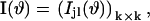 defined as
  are finite, and I(ϑ) is a positive-definite for all ϑ ∈ S(ϑ*).
VI. There exist functions Mijl(t) for which
 such that
Auxiliary statements
If the regularity criteria (Conditions I–VI) are satisfied, the following statements have been shown to apply (29–31):
Statement 1
 |
Statement 2
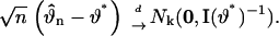 |
(Normal distribution with 0 mean and covariance I(ϑ*)−1.) A corollary of Statement 2 is that 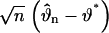 is stochastically bounded.
Statements 3, 4, and 5
Statement 3
Suppose that regularity criteria (Conditions I–VI) are satisfied for all ϑ ∈ S(ϑ*). Then,
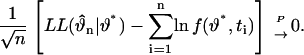 |
Proof
Expanding  into a Taylor series with respect to
  around the true parameter ϑ*,
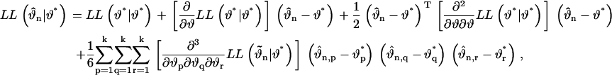 |
where  is a point on the line connecting
  and ϑ*. Because
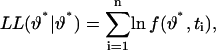
 |
and
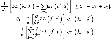 |
Because the random variable  has zero mean (by Condition IV) and finite variance (by Condition III), the average
  converges almost everywhere to zero, whereas
  is stochastically bounded (by Statement 2). Thus,
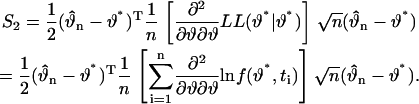 |
Because the random matrix  has finite mean (by Condition V), the average
 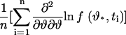 converges in distribution to −I(ϑ*); while
  is stochastically bounded (by Statement 2) and
 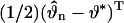 converges almost everywhere to zero (by Statement 1). Thus,
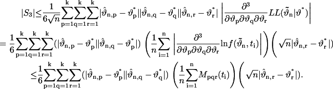 |
Because, by Condition VI, 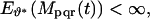 the average
 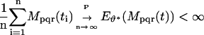 ; thus, both
 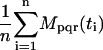 and
and 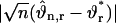 are stochastically bounded, whereas
 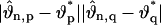 converges almost everywhere to zero. Thus,
  which concludes the proof.
Notes
Because, by the central limit theorem, 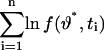 is asymptotically normally distributed with mean and variance given by Eqs. 5 and 6, Statement 3 implies the same for
The online Supplementary Material contains the demonstration that Conditions I–VI apply to the closed-time distributions of Schemes 1 and 2 (and 4), and 1R (and 2R, 4R).
Statement 4
Let  and let ΩR be a closed subset of Ω such that
  Let p:Φ→ΩR be a parameterization of ΩR, where Φ is a closed subset of
  Let
Let  denote the ML estimate based on t1,t2,…tn restricted to Φ; i.e.,
  ; and let
  denote
Suppose that the following conditions apply:
VII. There exists a unique point ϕ* ∈ Φ, such that
 is stochastically bounded. (Let
  denote p(ϕ*). Note that Condition VII implies
  )
)VIII. In an open convex neighborhood G(ϕ*) ⊂ Φ, containing ϕ*, there exist continuous first partial derivatives of f(p(ϕ),t) with respect to ϕ.
IX.
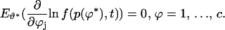
X. There exist functions
 and
and  continuous,
  h(0) = 0, such that
  for i, j = 1, …, k, for all ϕ ∈ G(ϕ*).
Then, 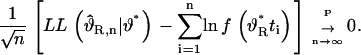
Proof
Differentiating 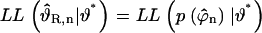 with respect to
  around the parameter ϕ*,
 |
where  is a point on the line connecting
  and ϕ*. Thus,
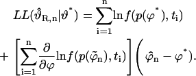 |
Therefore,
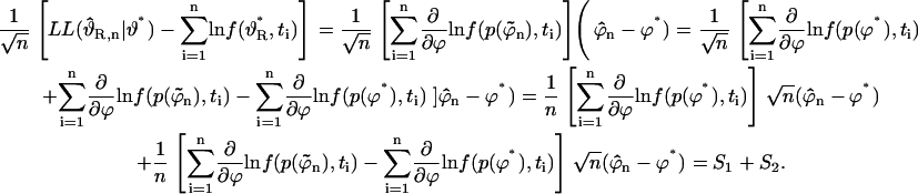 |
Thus,
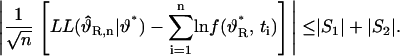 |
Because the random variable  has zero mean (by Condition IX), the average
 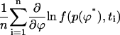 converges to zero in probability, whereas
 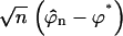 is stochastically bounded (by Condition VII). Thus,
On the other hand, applying Condition X,
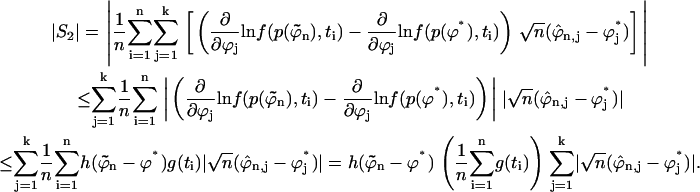 |
Because 
 ; thus, both
  and
and  are stochastically bounded. Because
  (by Condition VII),
  Thus,
Thus,  which concludes the proof.
Notes
Because, by the central limit theorem,  is asymptotically Gaussian distributed with mean and variance given by Eqs. 7 and 8, Statement 4 implies the same for LL
It is easy to show that Conditions VII–X apply if the reduced scheme predicts a single-exponential distribution (such as Schemes 1R, 2R, and 4R). The corresponding parameterization p will be  for the case of Scheme 1 versus 1R, and
  for the case of Scheme 2 versus 2R, with ΩR chosen as in Fig. 3 F.
Check VII. If the set of data t1,t2,…tn, regardless of its true distribution, is fitted to f(t) = (1/ϕ)e−t/ϕ by maximum likelihood, then
 (2). By the strong law of large numbers (as the random variables ti have finite variance),
  converges almost everywhere to the mean E(t) of the true distribution, thus ϕ* = E(t). By the central limit theorem,
  and is thus stochastically bounded.
Check VIII.
 which exists for all ϕ > 0.
- Check IX.
 therefore,
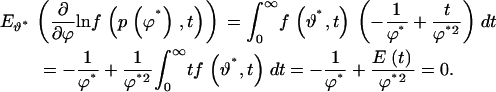
- Check X. Let ɛ < ϕ*, define G(ϕ*) as the open interval (ϕ* − ɛ, ϕ* + ɛ). Then, for all ϕ ∈ G(ϕ*),
Thus, h(x) = |x|, and g(t) has the form g(t) = a + bt. Trivially,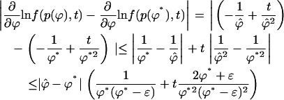

If the reduced model still contains more than one exponential component, the demonstration of Condition VII is less straightforward. However, simulations using Scheme 3, followed by ML-fits of the closed-time distribution to Scheme 3R, have confirmed that even if a five-component distribution is fitted with a four-component pdf the constrained fits converge to a unique point in ΩR with increasing events list length. The set of parameters printed in Fig. 1 for Scheme 3R corresponds to this experimentally determined ϕ*.
Statement 5
Let ΩR be a closed subset of Ω such that ϑ* ∉ ΩR. Suppose that Conditions I–VI are satisfied on S(ϑ*), and Conditions VII–X are satisfied on G(ϕ*). Then,
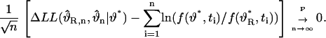 |
Proof
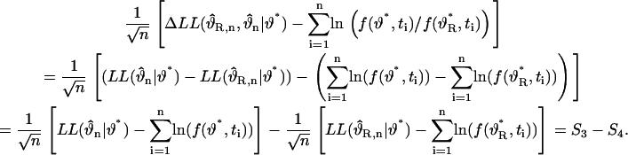 |
As  by Statement 3, and
  by Statement 4, this concludes the proof.
Notes
Because, by the central limit theorem, 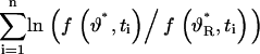 is asymptotically Gaussian-distributed with mean and variance given by Eqs. 9 and 10, Statement 5 implies the same for
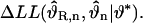
Statement 5 contains meaningful information only if ϑ* ∉ ΩR. If ϑ* ∈ ΩR (i.e., if the restricted model is the correct model), then  and
and 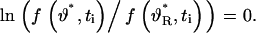 Therefore, in this case, Statement 5 reduces to the trivial statement
 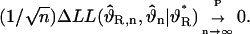 (This statement is obviously true as, by the χ2-theorem,
 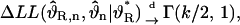 and is thus stochastically bounded.)
APPENDIX B: NUMERICAL IMPLEMENTATION OF EQS. 1–10
In practice, the integrals in Eqs. 1–10 are performed numerically between t = 0 (or t = tlow) and some t = thigh, where thigh is chosen such that the integrand vanishes for t > thigh. Because the integrand has the form  or
or  a choice of thigh could be, e.g., 100 times the longest time constant of
  However, because the longest time constants of the two pdfs might be very different, evaluation of one of the two pdfs might result in an underflow at high t, i.e., return zero; thus causing the algorithm to crash when attempting to take the logarithm. To avoid this problem the following simple strategy can be used. Both pdfs involved have the form
 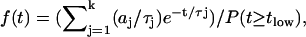 which can be rewritten in the form
 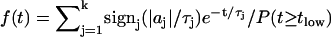 to allow for possible negative components such as in the closed-time pdf of Scheme 1. Define
  and
and 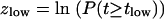 Then ln f(t) can be rewritten in the form of
  Because the term j corresponding to ymax always has a positive sign, the sum in the argument of the ln function will contain a term equal to +1, and thus will not underflow. Finally,
 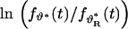 can be calculated as
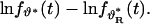
Abbreviations used: LL, log likelihood; ΔLL, log-likelihood ratio; E(X), expectation value of the random variable X; D2(X), variance of X; D(X), standard deviation of X; Ω, parameter space; Ξ, Θ, two different models, defined in terms of both scheme and parameter vector; ξ, ϑ, parameter vectors for models Ξ and Θ.
References
- 1.Colquhoun, D., and A. G. Hawkes. 1981. On the stochastic properties of single ion channels. Proc. R. Soc. Lond. B Biol. Sci. 211:205–235. [DOI] [PubMed] [Google Scholar]
- 2.Colquhoun, D., and F. J. Sigworth. 1995. Fitting and statistical analysis of single-channel records. In Single Channel Recording. B. Sakmann and E. Neher, editors. Plenum Press, New York.
- 3.Hamill, O. P., A. Marty, E. Neher, B. Sakmann, and F. J. Sigworth. 1981. Improved patch-clamp techniques for high-resolution current recording from cells and cell-free membrane patches. Pflugers Arch. 391:85–100. [DOI] [PubMed] [Google Scholar]
- 4.Sigworth, F. J., and S. M. Sine. 1987. Data transformations for improved display and fitting of single-channel dwell time histograms. Biophys. J. 52:1047–1054. [DOI] [PMC free article] [PubMed] [Google Scholar]
- 5.Rothberg, B. S., and K. L. Magleby. 1998. Kinetic structure of large-conductance Ca2+-activated K+ channels suggests that the gating includes transitions through intermediate or secondary states. A mechanism for flickers. J. Gen. Physiol. 111:751–780. [DOI] [PMC free article] [PubMed] [Google Scholar]
- 6.Horn, R., and K. Lange. 1983. Estimating kinetic constants from single channel data. Biophys. J. 43:207–223. [DOI] [PMC free article] [PubMed] [Google Scholar]
- 7.Ball, F. G., and M. S. Sansom. 1989. Ion-channel gating mechanisms: model identification and parameter estimation from single channel recordings. Proc. R. Soc. Lond. B Biol. Sci. 236:385–416. [DOI] [PubMed] [Google Scholar]
- 8.Qin, F., A. Auerbach, and F. Sachs. 1996. Estimating single-channel kinetic parameters from idealized patch-clamp data containing missed events. Biophys. J. 70:264–280. [DOI] [PMC free article] [PubMed] [Google Scholar]
- 9.Fredkin, D. R., and J. A. Rice. 1992. Maximum likelihood estimation and identification directly from single-channel recordings. Proc. Biol. Sci. 249:125–132. [DOI] [PubMed] [Google Scholar]
- 10.Colquhoun, D., A. G. Hawkes, and K. Srodsinski. 1996. Joint distributions of apparent open times and shut times of single ion channels and the maximum likelihood fitting of mechanisms. Philos. Trans. R. Soc. Lond. A. 354:2555–2590. [Google Scholar]
- 11.Colquhoun, D., C. J. Hatton, and A. G. Hawkes. 2003. The quality of maximum likelihood estimates of ion channel rate constants. J. Physiol. 547:699–728. [DOI] [PMC free article] [PubMed] [Google Scholar]
- 12.Rothberg, B. S., and K. L. Magleby. 1999. Gating kinetics of single large-conductance Ca2+-activated K+ channels in high Ca2+ suggest a two-tiered allosteric gating mechanism. J. Gen. Physiol. 114:93–124. [DOI] [PMC free article] [PubMed] [Google Scholar]
- 13.Rothberg, B. S., and K. L. Magleby. 2000. Voltage and Ca2+ activation of single large-conductance Ca2+-activated K+ channels described by a two-tiered allosteric gating mechanism. J. Gen. Physiol. 116:75–99. [DOI] [PMC free article] [PubMed] [Google Scholar]
- 14.Beato, M., P. J. Groot-Kormelink, D. Colquhoun, and L. G. Sivilotti. 2004. The activation mechanism of α1 homomeric glycine receptors. J. Neurosci. 24:895–906. [DOI] [PMC free article] [PubMed] [Google Scholar]
- 15.Burzomato, V., M. Beato, P. J. Groot-Kormelink, D. Colquhoun, and L. G. Sivilotti. 2004. Single-channel behavior of heteromeric α1β-glycine receptors: an attempt to detect a conformational change before the channel opens. J. Neurosci. 24:10924–10940. [DOI] [PMC free article] [PubMed] [Google Scholar]
- 16.Weiss, D. S., and K. L. Magleby. 1989. Gating scheme for single GABA-activated Cl− channels determined from stability plots, dwell-time distributions, and adjacent-interval durations. J. Neurosci. 9:1314–1324. [DOI] [PMC free article] [PubMed] [Google Scholar]
- 17.Jackson, M. B., B. S. Wong, C. E. Morris, H. Lecar, and C. N. Christian. 1983. Successive openings of the same acetylcholine receptor channel are correlated in open time. Biophys. J. 42:109–114. [DOI] [PMC free article] [PubMed] [Google Scholar]
- 18.Hatton, C. J., C. Shelley, M. Brydson, D. Beeson, and D. Colquhoun. 2003. Properties of the human muscle nicotinic receptor, and of the slow-channel myasthenic syndrome mutant ɛ-L221F, inferred from maximum likelihood fits. J. Physiol. 547:729–760. [DOI] [PMC free article] [PubMed] [Google Scholar]
- 19.Shelley, C., and D. Colquhoun. 2005. A human congenital myasthenia-causing mutation (ɛ-L78P) of the muscle nicotinic acetylcholine receptor with unusual single channel properties. J. Physiol. 564:377–396. [DOI] [PMC free article] [PubMed] [Google Scholar]
- 20.Schorge, S., S. Elenes, and D. Colquhoun. 2005. Maximum likelihood fitting of single channel NMDA activity with a mechanism composed of independent dimers of subunits. J. Physiol. 569:395–418. [DOI] [PMC free article] [PubMed] [Google Scholar]
- 21.Csanády, L., K. W. Chan, D. Seto-Young, D. C. Kopsco, A. C. Nairn, and D. C. Gadsby. 2000. Severed channels probe regulation of gating of cystic fibrosis transmembrane conductance regulator by its cytoplasmic domains. J. Gen. Physiol. 116:477–500. [DOI] [PMC free article] [PubMed] [Google Scholar]
- 22.Carson, M. R., S. M. Travis, and M. J. Welsh. 1995. The two nucleotide-binding domains of cystic fibrosis transmembrane conductance regulator (CFTR) have distinct functions in controlling channel activity. J. Biol. Chem. 270:1711–1717. [DOI] [PubMed] [Google Scholar]
- 23.Lin, Y. F., Y. N. Jan, and L. Y. Jan. 2000. Regulation of ATP-sensitive potassium channel function by protein kinase A-mediated phosphorylation in transfected HEK293 cells. EMBO J. 19:942–955. [DOI] [PMC free article] [PubMed] [Google Scholar]
- 24.Enkvetchakul, D., G. Loussouarn, E. Makhina, S. L. Shyng, and C. G. Nichols. 2000. The kinetic and physical basis of K(ATP) channel gating: toward a unified molecular understanding. Biophys. J. 78:2334–2348. [DOI] [PMC free article] [PubMed] [Google Scholar]
- 25.Yang, K., K. Fang, L. Fromondi, and K. W. Chan. 2005. Low temperature completely rescues the function of two misfolded K ATP channel disease-mutants. FEBS Lett. 579:4113–4118. [DOI] [PubMed] [Google Scholar]
- 26.Csanády, L., and V. Adam-Vizi. 2003. Ca2+- and voltage-dependent gating of Ca2+- and ATP-sensitive cationic channels in brain capillary endothelium. Biophys. J. 85:313–327. [DOI] [PMC free article] [PubMed] [Google Scholar]
- 27.Mak, D. O., and J. K. Foskett. 1997. Single-channel kinetics, inactivation, and spatial distribution of inositol trisphosphate (IP3) receptors in Xenopus oocyte nucleus. J. Gen. Physiol. 109:571–587. [DOI] [PMC free article] [PubMed] [Google Scholar]
- 28.Wald, A. 1943. Test of statistical hypotheses concerning several parameters when the number of observations is large. Trans. Am. Math. Soc. 54:426–482. [Google Scholar]
- 29.Rao, C. R. 1973. Linear Statistical Inference and its Applications. John Wiley & Sons, New York.
- 30.Cox, D. R., and D. V. Hinkley. 1973. Theoretical Statistics. Chapman & Hall, New York.
- 31.Móri, F. T., and J. G. Székely. 1986. The maximum-likelihood method. In Multivariate Statistical Analysis. Mûszaki Könyvkiadó, Budapest, Hungary. 297–317.
- 32.Horn, R. 1987. Statistical methods for model discrimination. Applications to gating kinetics and permeation of the acetylcholine receptor channel. Biophys. J. 51:255–263. [DOI] [PMC free article] [PubMed] [Google Scholar]
- 33.Akaike, H. 1974. A new look at the statistical model identification. IEEE Trans. Autom. Control. AC19:716–723. [Google Scholar]
- 34.Schwarz, G. 1978. Estimating the dimension of a model. Ann. Stat. 6:461–464. [Google Scholar]
- 35.Blunck, R., U. Kirst, T. Riessner, and U. Hansen. 1998. How powerful is the dwell-time analysis of multichannel records? J. Membr. Biol. 165:19–35. [DOI] [PubMed] [Google Scholar]
- 36.Press, W. H., W. T. Vetterling, S. A. Teukolsky, and B. P. Flannery. 1992. Numerical Recipes in C. The Art of Scientific Computing. Cambridge University Press, Cambridge, UK.
- 37.L'Ecuyer, P. 1988. Efficient and portable combined random number generators. Commun. ACM. 31:742–749. [Google Scholar]
- 38.Knuth, D. E. 1981. Seminumerical algorithms. In The Art of Computer Programming. Addison-Wesley, Reading, MA.
- 39.Caceci, M. S., and W. P. Cacheris. 1984. Fitting curves to data. The simplex algorithm is the answer. Byte May:340–348.
- 40.Chernoff, H. 1954. On the distribution of the likelihood ratio. Annu. Math. Stat. 25:573–578. [Google Scholar]
- 41.Kudo, A. 1963. A multivariate analogue of the one-sided test. Biometrika. 50:403–418. [Google Scholar]
- 42.Nuesch, P. E. 1966. On the problem of testing location in multivariate populations for restricted alternatives. Annu. Math. Stat. 37:113–119. [Google Scholar]
- 43.Shapiro, A. 1985. Asymptotic distribution of test statistics in the analysis of moment structures under inequality constraints. Biometrika. 72:133–144. [Google Scholar]
- 44.Self, S. G., and K. Y. Liang. 1987. Asymptotic properties of maximum likelihood estimators and likelihood ratio tests under nonstandard conditions. J. Am. Stat. Assoc. 82:605–610. [Google Scholar]
- 45.McManus, O. B., and K. L. Magleby. 1989. Kinetic time constants independent of previous single-channel activity suggest Markov gating for a large conductance Ca-activated K channel. J. Gen. Physiol. 94:1037–1070. [DOI] [PMC free article] [PubMed] [Google Scholar]
- 46.Neelands, T. R., L. J. Greenfield, Jr., J. Zhang, R. S. Turner, and R. L. Macdonald. 1998. GABAA receptor pharmacology and subtype mRNA expression in human neuronal NT2-N cells. J. Neurosci. 18:4993–5007. [DOI] [PMC free article] [PubMed] [Google Scholar]
- 47.Obejero-Paz, C. A., S. W. Jones, and A. Scarpa. 1998. Multiple channels mediate calcium leakage in the A7r5 smooth muscle-derived cell line. Biophys. J. 75:1271–1286. [DOI] [PMC free article] [PubMed] [Google Scholar]
- 48.Obejero-Paz, C. A., M. Auslender, and A. Scarpa. 1998. PKC activity modulates availability and long openings of L-type Ca2+ channels in A7r5 cells. Am. J. Physiol. 275:C535–C543. [DOI] [PubMed] [Google Scholar]
- 49.Li, J., and H. A. Lester. 1999. Single-channel kinetics of the rat olfactory cyclic nucleotide-gated channel expressed in Xenopus oocytes. Mol. Pharmacol. 55:883–893. [PubMed] [Google Scholar]
- 50.Haas, K. F., and R. L. Macdonald. 1999. GABAA receptor subunit γ-2 and δ-subtypes confer unique kinetic properties on recombinant GABAA receptor currents in mouse fibroblasts. J. Physiol. 514:27–45. [DOI] [PMC free article] [PubMed] [Google Scholar]
- 51.Hallermann, S., S. Heckmann, J. Dudel, and M. Heckmann. 2005. Short openings in high resolution single channel recordings of mouse nicotinic receptors. J. Physiol. 563:645–662. [DOI] [PMC free article] [PubMed] [Google Scholar]
- 52.Celentano, J. J., and A. G. Hawkes. 2004. Use of the covariance matrix in directly fitting kinetic parameters: application to GABAA receptors. Biophys. J. 87:276–294. [DOI] [PMC free article] [PubMed] [Google Scholar]
- 53.Horn, R., and C. A. Vandenberg. 1984. Statistical properties of single sodium channels. J. Gen. Physiol. 84:505–534. [DOI] [PMC free article] [PubMed] [Google Scholar]
- 54.Korn, S. J., and R. Horn. 1988. Statistical discrimination of fractal and Markov models of single-channel gating. Biophys. J. 54:871–877. [DOI] [PMC free article] [PubMed] [Google Scholar]
- 55.Ding, S., and F. Sachs. 1999. Single channel properties of P2X2 purinoceptors. J. Gen. Physiol. 113:695–720. [DOI] [PMC free article] [PubMed] [Google Scholar]
- 56.Michels, G., F. Er, I. Khan, M. Sudkamp, S. Herzig, and U. C. Hoppe. 2005. Single-channel properties support a potential contribution of hyperpolarization-activated cyclic nucleotide-gated channels and If to cardiac arrhythmias. Circulation. 111:399–404. [DOI] [PubMed] [Google Scholar]
- 57.Milescu, L. S., G. Akk, and F. Sachs. 2005. Maximum likelihood estimation of ion channel kinetics from macroscopic currents. Biophys. J. 88:2494–2515. [DOI] [PMC free article] [PubMed] [Google Scholar]