The use of QSD (q-sequence deconvolution) to recover superposed, transient evoked-responses

Abstract

Objective: We describe q-sequence deconvolution (QSD), a new data acquisition/analysis method for evoked-responses that solves the problem of waveform distortion at high stimulus repetition-rates, due to response overlap. QSD can increase the sensitivity of clinically useful evoked-responses because it is well known that high stimulus repetition-rates are better for detecting pathophysiology.

Methods: QSD is applicable to a variety of experimental conditions. Because some QSD-parameters must be chosen by the experimenter, the underlying principles and assumptions of the method are described in detail. The theoretical and mathematical bases of the QSD method are also described, including some equivalent computational formulations.

Results: QSD was applied to recordings of the human auditory brainstem response (ABR) at stimulus repetition-rates that overlapped the responses. The transient ABR was recovered at all rates tested (highest 160/s), and showed systematic changes with stimulus repetition-rate within a single subject.

Conclusions: QSD offers a new method of recovering brain evoked-response activity having a duration longer than the time between stimuli.

Significance: The use of this new technique for analysis of evoked responses will permit examination of brain activation patterns across a broad range of stimulus repetition-rates, some never before studied. Such studies will improve the sensitivity of evoked-responses for the detection of brain pathophysiology. New measures of brain activity may be discovered using QSD. The method also permits the recovery of the transient brain waveforms that overlap to form ‘steady-state’ waveforms. An additional benefit of the QSD method is that repetition-rate can be isolated as a variable, independent of other stimulus characteristics, even if the response is a nonlinear function of rate.

1. Introduction

It is well known that evoked responses can detect pathology more readily if the stimulus repetition-rate is high. For example, Hecox et al. (1981) stated that for pediatric applications of the auditory brainstem response (ABR), “…increasing rate of stimulation facilitates the identification of [ABR] abnormalities”. As late as 2002, the use of high-rate stimuli has been strongly advocated for the ABR when evaluating preterm infants (Jiang et al., 2002). (see the Discussion and Table 1 for additional, extensive evidence for the known value of using a high stimulus repetition-rate to detect brainstem disorders.)

Table 1.

References in which one or more patients showed an abnormal ABR at faster stimulus repetition-rates, but had a normal ABR at low repetition-rates. The low-rate ABR gave an undesirable false negative result in these patients. Pathologies are ordered by the year of earliest report.

Brainstem tumors and acoustic neuromas	Daly et al. (1977) and Tanaka et al. (1996)
Demyelinating diseases, such as multiple sclerosis	Robinson and Rudge (1977b,c), Stockard and Rossiter (1977), Stockard and Sharbrough (1977), Elidan et al. (1982), Collette et al. (1984), Keith and Jacobson (1985) and Jacobson et al. (1987)
Downs syndrome and similar conditions	Van Olphen et al. (1979) and Uri et al. (1984)
IVth ventricle epidermoid tumor	Yagi and Kaga (1979)
Closed head injuries	Hecox et al. (1981), Hecox and Burkard (1982) and Abd-al-Hady et al. (1990)
Pontine glioma, spinocerebellar degeneration, Wilson's disease	Fujita et al. (1981)
Ischemic lesions	Gerling and Finitzo (1983)
Bell's palsy	Uri et al. (1984)
AIDS in infants and children	Frank et al. (1992)
Purulent meningitis (long-term follow-up)	Jiang (1999)
Neonatal asphyxia	Jiang et al. (2001)
Hyperlipidemia	Zhang and Wang (2002)
Mercury exposure	Counter (2003)

Despite strong evidence for the usefulness of high-rate stimulation, technical difficulties prevent its widespread use. “Unfortunately, the clarity of the [ABR] often deteriorates as stimulation rate is increased” (Weber and Fujikawa, 1977). Similarly “Faster rates (more than 80 per second) have rate-dependent abnormalities in our experience, but use of such rapid rates of stimulation is self-defeating in some cases because of the associated loss of [ABR] resolution and interpretability” (Stockard et al., 1980). The deterioration of waveshape with increasing stimulus repetition-rate has been repeatedly observed (Don et al., 1977; Jewett and Williston, 1971; Kjaer, 1980; Starr and Brackmann, 1979; Stockard et al., 1978, 1983). Such deterioration affects waveform identification: “…high rates of stimulation do result in increased difficulty in wave identification…” (Harkins et al., 1979), which, in turn, affects clinical usefulness: “The relative difficulty of waveform recognition at 70 clicks per second, with increased waveform duration and indistinct peaks, restricted the clinical utility of that stimulus rate” (Chiappa et al., 1980).

One cause for deterioration of the ABR waveform with increased stimulus rate was explained by Kjaer (1980): “When fixed ISIs are used, potentials in the sampling time will systematically be contaminated by later components of the [Auditory Evoked Potential]…and as this contamination is time-locked to the stimulus, it cannot become attenuated by averaging”. Of the ABR, Zollner et al. (1976) said: “Higher click rates than 100/sec could not be used, because of the superposition of the first potential with the fifth one”. This overlap has been repeatedly observed (Eysholdt and Schreiner, 1982; Hyde et al., 1976; Pratt et al., 1986; Robinson and Rudge, 1977a).

We have developed a new method, q-sequence deconvolution (QSD), to deal specifically with the problem of responses that have a duration greater than that of the SI (stimulus interval start-to-start). We predict that QSD will improve the sensitivity of clinical tests that utilize evoked-responses, including those for newborn screening. In addition, QSD will permit study of brain functions that depend upon higher stimulus repetition-rates than can be studied by present techniques.

QSD is based upon computer averaging, utilizing the advantage of modern hardware to average continuously, without pause (i.e. with a 100% duty cycle). The consequence is that, with enough sweeps, the resultant average is a circular vector (where the last data point in the average not only follows the next-to-last point, but also precedes the first data point). This circularity permits frequency-domain computations with the following advantages: (1) there is no necessity of windowing time-domain data, (2) flexible filtering is available, and (3) deconvolution is accomplished by division. These advantages are utilized in the QSD method.

QSD can be used to recover transient evoked-responses because these responses are generated by sequentially activated neuronal sources. The physics of volume conductors requires that when different sources are simultaneously active, response superposition will occur on each data channel. (An experimental example of the summation of potentials from different far-field current sources is shown in Fig. 9 of the first cat ABR paper, Jewett, 1970.) Summed-data-waveforms that are composed of superposed transient responses are subject to misinterpretation when stimulus repetition-rate is varied. For example, even though the transient response is unchanged by changing the repetition-rate, the algebraic summation of the superposed transient responses may appear as an enhanced ‘oscillation’ if peaks happen to add to peaks, whereas if peaks happen to add to valleys, then the response will appear diminished.

A crucial aspect of QSD is the carefully chosen ‘q-sequence’ that determines the stimulus-timing pattern. If the stimulus timing-pattern is precisely periodic (i.e. it does not jitter), then it is not mathematically possible to derive a unique transient response to each stimulus from the superposed signal (there are more unknown variables than simultaneous equations). On the other hand, if the stimulus-timing pattern is jittered, we will show that the single-stimulus response-waveform can be fully recovered from noise-free superposed data. The inevitable presence of noise means that not all ‘jitters’ are useful—the devil is in the details of selecting the timing-pattern of the stimulus-sequence.

In practice, q-sequences with a small amount of jitter are used. One reason is diagrammed in Fig. 1, which shows a hypothetical nonlinear relationship between SI (stimulus interval start-to-start) and some measure of an evoked-response waveform. That measure might be latency, or amplitude, or some other measure; the exact detail is not critical. Let us assume that the measurement occurs at some post-stimulus time τ. Three ‘point-estimates’ of the measure of the evoked response, each from a different run, are labeled b_A(τ), b_B(τ), and b_C(τ) in Fig. 1. The subscripts of b(τ) indicate that these are different waveforms associated with the different runs, where the differences are due to the mean repetition-rate of the SI, all other parameters being held constant. These point-estimates are just a few of those needed to establish the shape of the nonlinear relationship. The point-estimates are obtained from repeated runs that sample different SI ranges (marked as jA, jB, and jC). In Fig. 1, the range-limits have been chosen to be ±7% of the mean value for each run for illustrative purposes. If the output variation is small, the errors in the point-estimate will also be small (see Discussion). So, an estimate of the global nonlinearity can be obtained from repeated local estimates, each recovered using a separate run. Clearly, the jitter needs to be smaller in regions with a high slope, as compared with low-slope regions, to reduce distortions that can occur from inclusion of different waveshapes in the superposed data.

Fig. 1.

Hypothetical relationship between the immediately preceding SI and some measure derived from an evoked-response waveform. We assume that the measurement is at a single point on the waveform, at time τ. Three ‘point estimates’, b_A(τ), b_B(τ), and b_C(τ) are derived from 3 different data-runs, each with a different mean SI, and with a different absolute range of jitter (jA, jB, jC). The percentage jitter in this example is ±7% of the mean SI for each run. Note that because of the shape of the nonlinear curve, the ±7% jitter yields about the same range of variation of output for all runs. This would not be true if the nonlinearity curve was a different shape with its larger slopes at larger SI.

When using QSD, the goal is to minimize waveshape differences by decreasing SI jitter, i.e. to choose a q-sequence that approximates to periodicity. Hence, the stimulus timing-sequences of QSD are quasi-periodic. (The first letters of ‘q-sequence’, ‘QSD’, and ‘quasi-periodic’ can be used as a mnemonic to recall this important characteristic of the stimulus timing-sequences.) The quasi-periodic, small-jitter sequences used in QSD differ significantly from large-jitter pseudo-random sequences such as maximum-length sequences (MLS) (see Discussion).

The new terminology and acronyms used in this paper are listed and defined in Appendix D as an aid to the reader. QSD was previously called WAAD (see Appendix D) in some presentations of this work: an unscheduled talk at the 2001 Vancouver meeting of the International Evoked Response Audiometery Study Group, and as posters (Jewett, 2002; Jewett et al., 2002, 2003).

2. QSD method

2.1. Overall view of the QSD process

In Fig. 2 the QSD process is diagrammed as a flow chart. The figure also shows symbols that will later be used in descriptive equations. The sequence control element in Fig. 2 continuously and repeatedly outputs a quasi-periodic finite-length circular timing-sequence, which is a binary series of ones and zeros. The timing-sequence is a circular vector where it is useful to express time as an angle. Hence the timing-sequence is symbolized by q(θ). In the circular vector, θ ranges from 0 to 2π–Δ (where Δ is the minimum time discretization, expressed as an angle in radians). The duration of the timing-sequence is the sequence length (SL), with units of either time or angle.

Fig. 2.

Diagram of the overall scheme of use of QSD. Terms are defined below and also in Appendix D. A–D, analog-to-digital; b, brain response (on a single data channel); Δ, the smallest time-interval in the circular vectors, expressed as an angle; n, noise; e, subscript indicating those experimental parameters that are held constant within any given run, but which can cause between-run differences in waveshape; q, quasi-periodic timing-sequence; SL, sequence length; θ, time on a circular vector, expressed as an angle, in radians; v, voltage (on a single data channel).

The waveform generator turns each ‘one’ in the binary timing-sequence into an analog waveform. While the analog waveforms are identical, the timing of the waveforms from start-to-start is not uniform due to the jitter in q(θ). Each analog waveform is then transduced into an appropriate stimulus, such as a sound, a light, a vibration, etc. The final result is a sequence of stimuli that activates the central nervous system (CNS), which we will treat as a ‘black box’ whose inner workings are not directly observable.

For didactic purposes we assume that when the CNS is stimulated by each stimulus in the sequence, the same evoked-response is generated, symbolized by b_e(θ). Note that the e subscript indicates that b_e(θ) is a function of the experimental conditions under which the data are collected, such as mean stimulation rate, stimulus intensity, other stimulus characteristics, manner of stimulus delivery, subject's attentional state, presence of distracting or masking stimuli, time of day, presence of drugs, etc. It is assumed that these parameters do not vary within the data-run, though they may well vary between data-runs. It is further assumed that if there is adaptation in the brain's response, then b_e(θ) is the response when the adaptation has asymptoted. If the duration of the evoked-response b_e(θ) is greater than the SI, the evoked responses will temporally overlap, as shown by the dotted waveforms labeled ‘b_e(θ) overlapped’ in Fig. 2. If such overlap is algebraically summed on a given data channel, superposition of these waveforms occurs (solid line labeled ‘v_e(θ) superposed’ in Fig. 2). The voltage on a single channel ${\tilde{v}}_{\mathrm{e}}\left(\theta \right)$ includes the superposed v_e(θ) and noise, n_e(θ). ${\tilde{v}}_{\mathrm{e}}\left(\theta \right)$ is circular if the recording has been averaged with a 100% duty cycle synchronized with each repetition of the circular q-sequence. Such synchronization is indicated in Fig. 2, and can occur either through a recording passed through the A–D converter, or by a direct synch-pulse each q-sequence cycle.

From now on, to make reading easier, the ‘e’ subscript will be dropped from the text and equations, at the risk of forgetting that the values represented by these symbols can be affected by experimental conditions. We first consider the noise-free case. The brain response, b(θ), can be recovered if the jittered-timing of the q sequence, q(θ), carries through to the channel-signal, v(θ). Recovery of b(θ) can be accomplished by deconvolution since, as we will show, the summed overlap of b(θ) with the temporal pattern of q(θ) is equivalent to convolution of b(θ) with q(θ) under the following conditions:

1. b(θ) does not vary with the SIs in the jittered stimulation-sequence, and

2. q(θ) is expressed as ones and zeros.

In order to provide an understanding of this assertion, we will first diagram the process, and then present the mathematics.

Fig. 3 shows q(θ), b(θ), and v(θ) as circular vectors. Because these vectors are circular, the timing is expressed as an angle (θ) relative to some zero time (θ=0). This convention will be used throughout this paper. The A–D timing is shown on the bottom circular ‘data register’ v(θ). On the other two rings, the same A–D timing occurs, but is not shown so as to avoid diagram-clutter. In Fig. 3 the stimuli in the circular timing-sequence, q(θ), occur 11 times (numbered 0–10). The first stimulus is activated at time θ=0 and that stimulus is labeled ‘0’. Since the timing-sequence is circular, the stimulus-times can be numbered either forward in time (positive numbers for successive stimulations), or backward in time (negative numbers for prior stimulations).

Fig. 3.

Diagram of relationships of the circular vectors of QSD. Stimulus locations on q(θ) are numbered in both positive (counter-clockwise) and negative (clockwise) directions.

In the explanation that follows, the upper and lower rings will remain fixed, while the middle ring will be imagined to rotate. Assume that the 0 stimulus, at time θ=0, generates the evoked-response waveform b(θ) in the middle ring, and imagine adding that waveform, at that position, into the empty circular data-register v(θ). At the next stimulus (1), the same b(θ) waveform is generated, but it is now time-shifted before being added into v(θ). That is, the middle ring can be imagined to have been rotated counter-clockwise so that the start (θ=0) of the b(θ) ring now aligns with 1 in the q(θ) ring. After this imagined shift, the b(θ) waveform is algebraically added into the contents of v(θ). When the same process of shift and add is completed for each of the stimuli in q(θ), v(θ) will be the algebraic summation of b(θ) overlapped in accordance with the timing of q(θ).

Note that the same summation in v(θ) is obtained by a single complete cycle of q(θ) in the reverse direction (negative-numbered stimuli). The reverse-direction approach is useful if one asks ‘what voltages have contributed to a specific point in the v(θ) data register?’ The answer is that the voltage at any one point in v(θ) is the sum of the voltage from the response b(θ) to the most-recent stimulus, added to a longer-latency point in b due to the response to the previous stimulus (increased negative stimulus number), plus the even-longer-latency voltage in b(θ) in response to the even-earlier stimulus (more negative stimulus number), etc. Since the summation of all responses in v(θ) is the same no matter the direction taken, whether one takes the view that the ‘present filled-vector is due to summation of responses to a series of past stimuli’ (a time-reversed view) or that the ‘present empty-vector will be filled as responses to the stimulus sequence are summed’ (a time-forward view) is a matter of personal preference.

2.2. Mathematical description

In Appendix C.1 we show that the sum of algebraically overlapped evoked responses v(θ) is mathematically identical to the convolution of the single evoked-response b(θ) with the timing-sequence q(θ). Hence, the process diagrammed in Fig. 3 can be mathematically described as a time-domain circular convolution:

$$v\left(\theta \right)=b\left(\theta \right)\copyright q\left(\theta \right)$$ (1)

where © is circular convolution and q(θ) is limited to the binary digits 1 and 0. So long as there is no noise, b(θ) is recoverable by the inverse operation of circular deconvolution of v(θq) by q(θ).

The situation becomes more complicated as we allow for noise, as given by Eq. (2):

$$\tilde{v}\left(\theta \right)=\left[b\left(\theta \right)\copyright q\left(\theta \right)\right]+n\left(\theta \right)$$ (2)

By definition, noise is uncorrelated with the timing of the stimuli, and is, thus, independent of b(θ). Sources of noise include uncorrelated brain activity, muscle artifacts, non-biological noise from amplifiers, ambient electrical activity in the recording environment, and unknown causes that disappear after a few experiments. All noise sources are included, for our purposes, in n(θ). The tilde symbol, as we use it, implies ‘with noise added’, hence $\tilde{v}\left(\theta \right)$, and later, b̃(θ).

There are constraints on q-sequences in both the time-domain and the frequency-domain, which will be described in detail later. To introduce the frequency-domain constraints, we transform Eq. (2) to the frequency domain:

$$\tilde{V}\left(f\right)=\left[B\left(f\right)\mathcal{Q}\left(f\right)\right]+N\left(f\right)$$ (3)

(Note: throughout this paper, an upper-case letter indicates Fourier coefficients in the frequency-domain expressed as a complex number.) If both vectors, b(θ) and q(θ), are circular and of the same length, then time domain convolution is equivalent to multiplication in the frequency-domain. Hence, B(f) is multiplied by $\mathcal{Q}\left(f\right)$ within the brackets, $\mathcal{Q}\left(f\right)$ being the complex Fourier coefficient of the timing-sequence q(θ). To calculate the estimated brain response B̃(f), we deconvolve in the frequency-domain, i.e. we divide our observed, recorded data $\tilde{V}\left(f\right)$ by $\mathcal{Q}\left(f\right)$:

$$\tilde{B}\left(f\right)=\frac{\tilde{V}\left(f\right)}{\mathcal{Q}\left(f\right)}=\frac{B\left(f\right)\mathcal{Q}\left(f\right)}{\mathcal{Q}\left(f\right)}+\frac{N\left(f\right)}{\mathcal{Q}\left(f\right)}$$ (4)

It is apparent from Eq. (4) that deconvolution returns the signal since $\mathcal{Q}\left(f\right)$ in the denominator cancels $\mathcal{Q}\left(f\right)$ in the numerator with regard to B(f). But B̃(f) will also contain noise having the magnitude N(f)/Q(f). It is also apparent from Eq. (4) that $\mathcal{Q}\left(f\right)$ must not be zero.

2.3. The effects of N(f)/Q(f) on the usefulness of QSD

The last term of Eq. (4) is very significant in whether QSD can be successfully used. This is most easily understood if the Fourier coefficients are thought of in polar coordinates, so that we can distinguish magnitude and phase. As will become clear, the magnitude of $\mathcal{Q}\left(f\right)$, symbolized by |Q(f)|, is critical in the successful use of QSD because $\mathcal{Q}\left(f\right)$ is in the denominator in Eq. (4). The consequence is that if the magnitude of |Q(f)| is less than unity, then whatever noise is present after averaging will be increased during deconvolution. Increasing noise is undesirable, and can be, at times, fatal to efforts to detect a usable signal. This leads us to judge a timing-sequence as either ‘usable’ or ‘unusable’ based upon on whether there are any less-than-unity Q-magnitudes in the passband. The reason that ‘passband’ is specified is that, as we will show later, a sequence with a small amount of jitter will always have some frequencies that have less-than-unity Q-magnitudes. But if those low Q-magnitudes are outside the passband their effects can be filtered, whereas that is not possible in the passband. The equation for |Q(f)| is given in Appendix C.2 (Eq. (C4)).

To demonstrate the effects of the timing sequence on noise, in Fig. 4 we show two sets of Q-magnitudes ({|Q(f)|}), over a passband of 30–150 Hz. Each of the two sets of Q-magnitudes are based on different timing-sequences that have the same mean stimulus repetition-rate (42/s), with an SL of 500 ms. These two sets show the difference between what we call a ‘good sequence’ (i.e. usable), and a ‘bad sequence’ (i.e. unusable). The sequence in Fig. 4A has Q-magnitudes in the passband that are all greater than unity (unit-magnitude is shown by the horizontal dashed line). On the other hand, the sequence in Fig. 4B has only 3 Q-magnitudes greater than unity, the rest being in the range of about 0.01. With the linear ordinate of Fig. 4B it is not possible to see that the majority of magnitudes are not zero, so the same data are plotted on a logarithmic ordinate in Fig. 4B′. The timing-sequence shown in Fig. 4B and B′ was formed by taking an exactly periodic sequence and moving one stimulation point by one A–D point. Thus, it is almost uniform. If it had been completely uniform, the Q-magnitudes at frequencies between the ‘teeth’ of the ‘comb filter’ of Fig. 4B would have been zero, and the signal would not be detectable in ‘infinite’ noise.

Fig. 4.

Effect of Q-magnitudes upon noise after deconvolution. Two sequences (one ‘good’ usable and one ‘bad’ unusable) are shown, each with a passband of 30–150 Hz for a 42/s stimulus repetition-rate on an SL of about 500 ms (21 stimuli). A Q-magnitude of unity is marked by a dashed line in A, B, B′. (A) Q-magnitudes from a usable sequence, the timing of the q-sequence having been selected so that all values are greater than unity in the passband. (B) Q-magnitudes from an unusable sequence, which had uniform SI except for a single time-point difference on one interval. Note that most Q-magnitudes are less than unity in the passband. (B′) Same as in B, but plotted on a logarithmic ordinate. Note that the small values are not zero, but range between 0.01 and 0.001. (C) Original noise comparable to that in an average that contains a signal, obtained by averaging two-thousand 500 ms sweeps of EEG with a 100% duty-cycle, from an awake human, eyes open, without any stimuli. (D) After deconvolution of the average in (C) with the timing-sequence whose Q-magnitudes are shown in (A). (E) After deconvolution of the average in (C) with the timing-sequence whose Q-magnitudes are shown in B, B′. Note that the vertical scale is 100 times that of (C) and (D).

The effect of these timing sequences on non-convolved noise can be seen by comparing the results of deconvolving the same noise-data with the two sequences. EEG ‘noise’, recorded without stimulation, was averaged (Fig. 4C). The average was then transferred to the frequency-domain where it was deconvolved with the $\mathcal{Q}\left(f\right)$ from either timing-sequence, and then transformed back into time-domain waveforms (Fig. 4D and E). Fig. 4D shows the noise reduction that occurs when the ‘good’ sequence of Fig. 4A is used. In contrast, Fig. 4E shows that there is increased noise if the ‘bad’ sequence of Fig. 4B and B′ is used. Note that in Fig. 4E the vertical scale is 100 times greater than in Fig. 4Cǃ The deconvolved noise of Fig. 4E is about 100 times greater because many of the Q-magnitudes shown in Fig. 4B′ are about 0.01. The consequences of the difference in noise can be readily imagined by assuming that a signal was also present. (Recall that the signal can be fully recovered by either sequence, as described previously.) If the signal could be seen in Fig. 4D, it would be lost in Fig. 4E where the noise is over 100 times larger. The phenomenon shown in Fig. 4 justifies the generalization that in the use of QSD, the critical effect of the $\mathcal{Q}$-magnitudes of the q-sequence is upon the noise, not the signal. If a QSD-user is not aware that different sequences may have different effects on noise, even though those sequences have similar experimental parameters, then variation in experimental results may be inexplicable (as they were to us early in the development of QSD).

2.4. Selection of q(θ)

The timing-pattern of a q-sequence is defined by a rule set that contains both time-domain and frequency-domain constraints. Here is an annotated list of the constraints on q-sequences:

Time-domain constraints:

1. The desired mean SI.

2. The range of permitted jitter. This may not be symmetrical around the mean SI if the distribution is kurtotic.

3. The sequence length. The duration of the SL must be larger than the duration of the response to an individual stimulus. If this requirement is not met, the response to each stimulus will overlap upon itself with a uniform periodicity and will not be recoverable in such a region. The duration of SL also affects the length of a data-run (which is the SL times the number of sweeps averaged). A judicious choice of SL also can act to cancel 60 and 120 Hz interference when the SL is an odd multiple of 1/2 the period of 120 Hz and the number of sweeps averaged is always a multiple of 4.

4. The digitizing rate used in the timing-sequence. Too low a rate may make finding of q-sequences difficult or impossible, as described in Appendix A.

Frequency-domain constraints:

5. The passband of the evoked-response. This determines the frequencies at which the Q-magnitudes of $\mid \mathcal{Q}\left(f\right)\mid$ should be near, or above, unity.

6. No zero Q-magnitudes at any frequency used in the deconvolution.

7. The minimum acceptable Q-magnitude.

8. The maximum acceptable variation in Q-magnitudes.

In general, the passband must be specified so that the timing of q(θ) can be made to keep less-than-unity Q-magnitudes outside the passband. If this requirement is met, noise in the passband is never increased by the deconvolution, because all the Q-magnitudes in the passband are greater than unity. The reasons for constraints 6, 7, and 8 will be evident later in the text.

The problems in identifying and dealing with Q-magnitudes less than unity when using QSD cannot be avoided if the user wishes to minimize the amount of jitter. Minimal jitter implies that the quasi-periodic timing-sequence is close to pure periodicity, i.e. close to a uniform SI. A periodic timing-sequence (with identical SIs) will have frequencies between the teeth of the comb whose Q-magnitudes are zero. Any miniscule perturbation away from periodicity will result in these values increasing only slightly as is observed in Fig. 4B′, which results in some less-than-unity Q-magnitudes. If the experimental goal is to find a timing sequence with adequate Q-magnitudes within the passband with minimal jitter (i.e. a minimal movement away from periodicity), such a sequence may not be found even after an extensive search. The options then available to the QSD-user include (a) increasing the amount of jitter, (b) increasing the SL, (c) re-ordering the SIs in a given sequence (i.e. further sequence searching), and/or (d) reducing the passband. Additional discussion of these issues is found in Appendix A.

2.5. q(θ) search

There is no analytic method known to the authors for finding a time-domain binary q-sequence based upon the required rule set. Hence, we do an iterative numerical search to find a workable timing-sequence by repeated generation and testing of the Q-magnitudes of the $\{\mid \mathcal{Q}\left(f\right)\mid \}$ set in the passband (the Q-magnitudes are calculated from Eq. (C4) in Appendix C.2). The search for the timing-sequence is a multiple-variable constrained optimization, for which a variety of computational methods exist. The specific optimization technique used is not critical so long as it is resistant to being trapped in local minima. We have used simulated annealing (Press et al., 1992). Essentially, the simulated annealing technique repeatedly generates timing-sequences and selects those that minimize some user-defined ‘cost function’ within the prescribed constraints. In our studies, the cost function required that all the Q-magnitudes within the desired passband be equal-to, or greater-than, unity. Other cost functions can also be considered, such as those incorporating constraints 6, 7, and 8 above. The q-sequence search can also include user-defined restrictions on q(θ), such as including presence or absence of a specific timing pattern, interposed correlated stimuli, asymmetrical limits of jitter relative to the mean, short pauses, harmonic SI, and/or maximum Q-magnitude differences for adjacent frequencies.

2.6. The fundamental equations of QSD

We now continue our explanation of how b̃(θ) is computed. Note that Eq. (4) is based upon deconvolution of the entire set of Fourier frequencies. The frequencies inside the passband are greater than unity because we have searched for the q-sequence until that condition was met. But, if the jitter is minimal, there will be some frequencies outside the passband, in the stopbands, that are less than unity. We cannot afford to deconvolve at these frequencies without risking an increase of noise. So, the passband and stopband computations in the frequency-domain differ as a function of frequency. To describe the differences, we explicitly define mutually exclusive frequency bands which together encompass all the Fourier frequencies of (f):

• (f^P) indicates frequencies in the passband. The passband includes only the frequencies-of-interest.

• (f^S) indicates frequencies in the stopbands. The stop-bands include any transition frequencies.

The use of these mutually exclusive frequency bands has the consequence that the set of {B̃(f)} is made up of two components:

$$\left\{\tilde{B}\left(f\right)\right\}=\left\{\tilde{B}\left(f^{\mathrm{P}}\right)\right\}\cup \left\{\tilde{B}\left(f^{\mathrm{S}}\right)\right\}$$

When we expand this equation to show how each B̃ is obtained, we have the first of the 3 ‘fundamental equations of QSD’, as follows (Eq. (5)):

$$\left\{\tilde{B}\left(f\right)\right\}=\left\{\frac{\tilde{V}\left(f^P\right)}{\overleftrightarrow{\mathcal{Q}}\left(f^P\right)}\right\}\cup \left\{\frac{\tilde{V}\left(f^S\right)}{S\left(f^S\right)}\right\}$$ (5)

The implications of this equation are best understood by separating the variables according to the passband and stopband frequencies, to show what we hypothesize makes up each subset of $\left\{\tilde{V}\left(f\right)\right\}$. The remaining two ‘fundamental equations of QSD’ are: For passband frequencies:

$$\tilde{B}\left(f^{\mathrm{P}}\right)=\frac{B\left(f^{\mathrm{P}}\right)\mathcal{Q}\left(f^{\mathrm{P}}\right)}{\overleftrightarrow{\mathcal{Q}}\left(f^{\mathrm{P}}\right)}+\frac{N\left(f^{\mathrm{P}}\right)}{\overleftrightarrow{\mathcal{Q}}\left(f^{\mathrm{P}}\right)}$$ (6)

For stopband frequencies:

$$\tilde{B}\left(f^{\mathrm{S}}\right)=\frac{B\left(f^{\mathrm{S}}\right)\mathcal{Q}\left(f^{\mathrm{S}}\right)}{S\left(f^{\mathrm{S}}\right)}+\frac{N\left(f^{\mathrm{S}}\right)}{S\left(f^{\mathrm{S}}\right)}$$ (7)

where:

• $\mathcal{Q}\left(f\right)$ is determined solely by the q-sequence, being the effects of the convolution across all frequencies. Hence $\mathcal{Q}\left(f\right)$ is in both frequency bands: (f^P) and (f^S).

• $\overleftrightarrow{\mathcal{Q}}\left(f^{\mathrm{P}}\right)$ are the user-chosen passband Fourier coefficients used in the deconvolution, and are usually identical with $\mathcal{Q}\left(f^{\mathrm{P}}\right)$ so as to accurately recover the signal. The $\overleftrightarrow{\mathcal{Q}}$-magnitudes are usually greater than unity; for exceptions see the discussion below about ‘adjustments’.

• S(f^S) is the filter in the stopbands, and its value is very large at frequencies far from the passband, so as to make any effects of stopband-noise very small. In the transition frequencies adjacent to the passband, S(f^S) has values greater than the value of $\overleftrightarrow{\mathcal{Q}}\left(f^{\mathrm{P}}\right)$ at the passband edge.

The ‘fundamental equations of QSD’ illustrate the consequences of the method on the signal and the noise. Consider Eq. (6). This shows that in the passband, B(f^P) will be accurately computed since the quotient $\mathcal{Q}\left(f^{\mathrm{P}}\right)∕\overleftrightarrow{\mathcal{Q}}\left(f^{\mathrm{P}}\right)$ is unity. However, B̃(f^P) will still contain an error due to the quotient $N\left(f^{\mathrm{P}}\right)∕\overleftrightarrow{\mathcal{Q}}\left(f^{\mathrm{P}}\right)$. Since $1∕\overleftrightarrow{\mathcal{Q}}\left(f^{\mathrm{P}}\right)$ is less than one in the passband, passband noise is lessened as compared to its magnitude in the averaged data, $\tilde{V}\left(f^{\mathrm{P}}\right)$.

Eq. (7) shows that B̃(f^S) has two components outside the passband: the (undesired)brain response, and uncorrelated noise. Both components are attenuated (hopefully to small values) by S(f^S). The design of the stopband filtering should take into account that $\tilde{v}\left(t\right)$ is a circular vector.

After completing the calculations in the frequency-domain, the results are converted back to the timedomain. b̃(θ) is computed from the inverse discrete fourier transform (IDFT) using the combination of B̃(f^P) and B̃(f^S) to encompass all of the Fourier frequencies whose coefficients are non-zero. Alternative computational methods are described in Appendix B.

The reason for distinguishing between the two Q-magnitudes, $\mathcal{Q}\left(f^{\mathrm{P}}\right)$ and $\overleftrightarrow{\mathcal{Q}}\left(f^{\mathrm{P}}\right)$, in Eqs. (5)-(7) is that, although it is best that they be identical, they might not be identical if the user has ‘adjusted’ the magnitudes so as to obtain some signal-recovery despite a few ‘bad’ Q-magnitudes in the passband after exhaustive search. Adjustments can include changing a less-than-unity value of $\mid \overleftrightarrow{\mathcal{Q}}\left(f^{\mathrm{P}}\right)\mid$ at a specific frequency either to unity, or to a value similar to those of nearby frequencies. Another ‘adjustment’ might be not computing any values for a frequency in the passband at which the $\mathcal{Q}\left(f^{\mathrm{P}}\right)$ was small, or zero. Any adjustments will cause inaccuracies in the recovered waveform. Thus, these adjustments must be tested carefully for their effects and should be used sparingly.

The estimate of the brain waveform, b̃(θ), may differ from b(θ) for a number of reasons: From Eq. (6):

1. Residual noise from $N\left(f^{\mathrm{P}}\right)∕\overleftrightarrow{\mathcal{Q}}\left(f^{\mathrm{P}}\right)$. (This might have some systematic irregularity in the time-domain due to the unequal frequency-to-frequency magnitudes of $\overleftrightarrow{\mathcal{Q}}\left(f^{\mathrm{P}}\right)$, as shown in Fig. 4)

2. The $\overleftrightarrow{\mathcal{Q}}\left(f^{\mathrm{P}}\right)$ used in the deconvolution is not the identical at every (f) to $\mathcal{Q}\left(f^{\mathrm{P}}\right)$ due to adjustments for $\mathcal{Q}<1$.

From Eq. (7):

3. Residual brain activity in the stopband (especially the transition zone), whose magnitude has not been sufficiently reduced by the filter S(f^S) in the fraction $\left[B\left(f^{\mathrm{S}}\right)\mathcal{Q}\left(f^{\mathrm{S}}\right)\right]∕S\left(f^{\mathrm{S}}\right)$

4. Residual noise in the stopband (especially the transition zone), from noise not sufficiently reduced by the filter: N(f^S)/S(f^S).

From additional causes:

5. Additional (analog or digital) filtering of frequencies that are in b(θ).

6. Response variability in the average, probably due to systematic differences in the response as a function of the preceding SI or SIs.

7. Windowing of time-domain functions when analyzing non-averaged, non-circular data (not described in this paper).

3. Experimental examples: ABR recordings using QSD

3.1. Recording and analysis methods

Two young-adults, one of each gender, with normal hearing (by screening audiometer), gave informed consent according to an IRB-approved protocol. They sat in a comfortable recliner chair with a head rest in a dimly lit electrically shielded, sound-attenuating chamber. Potentials were recorded between vertex and ipsilateral earlobe electrodes. Recordings were plotted with vertex-positive up. The monaural 100 ms click stimuli were delivered by an Etymotic ER-2 insert-earphone. The A–D conversion rate was 48 kHz per channel using a Swissonic AD24 in 24 bit mode (a single sigma–delta A–D per channel). The SA Instruments preamplifier passband filter settings were 100–3000 Hz. Data were collected by a Mac G4 computer running MAX/MSP software (cycling74) for simultaneous stimulation and data acquisition. Data analysis included our own deconvolution program, and IGOR software (Wave-metrics) for display. The overall methodology was described previously: (1) time-domain averaging of the SL, (2) transfer of the data to the frequency-domain, (3) division of the data by the frequency-domain Fourier coefficients of the sequence in the passband, (4) conversion back to the time-domain.

All of the data runs were very long in order to minimize run-to-run variability (see Appendix C.3) in the comparisons. For the 55/s run, the run duration was 39 min, the number of stimuli 129,000, and the SL was 204 ms. For the other runs the duration was 15 min, and the number of stimuli were as follows (SL in ms when QSD was used): 9.6/s—8640 (no QSD); 40/s—36,000 (no QSD); 80/s—72,000 (388 ms); 120/s—108,000 (254 ms); 160/s—144,000 (196 ms).

The following parameters for the q-sequences were determined based upon system capabilities and preliminary experimentation:

1. A–D/D–A rate=48 kHz. (The A–D/D–A equipment was designed for music systems, to be compatible with compact-disk specifications, and does not imply that such a high rate is needed by QSD. Also see Appendix A.)

2. Sequence lengths=ranged from 196 to 388 ms because each was chosen to cancel 60 and 120 Hz.

3. Mean stimulus repetition-rates=55, 80, 120, 160 stimuli per second.

4. Maximum jitter=±12% of mean (an SI-ratio of 0.27; see Appendices A and D).

5. Waveform passband=120–2000 Hz.

6. Search cost function=all Q-magnitudes in passband>1.0.

Using a 50 MHz computer running Linux, the selection process using simulated annealing took several hours for each repetition-rate.

3.2. Recordings and comments

Data taken from the subjects are shown in Fig. 5. The stimuli were delivered to the insert-earphone at time 0, with the stimulus reaching the ear drum after an additional 1 ms delay from the tubing length. Only the first 10 ms of each sweep are shown, along with a 5 ms pre-stimulus baseline in Fig. 5B. Because of the circularity of the 100% duty-cycle averages, the pre-stimulus baseline is also the ‘end’ of the SL.

Fig. 5.

Auditory brainstem response (ABR) recordings from two subjects. Click stimuli delivered monaurally by Etymotic ER-2 insert-earphone at time ‘0’ so that the stimuli arrive at the eardrum 1 ms later, due to tube-delay. (A) ABR from male subject, clicks at 60 dbSL, at 55/s using a jittered sequence. The smallest SI in the sequence was 16 ms. The waveform found by QSD is the solid line. The dotted line is the 10 ms duration ‘standard’ average of the same data, triggered on each stimulus. The similarity of waveforms suggests that QSD returns the same waveform in a direct comparison (when there is no overlap). The passband was 120–2500 Hz. (B) Recordings from female subject, clicks intensity 65 dbSL (relative to threshold measured at slowest rate). Passband filtered from 120 to 2000 Hz during deconvolution. At 9.6/s and 40/s waveforms obtained by standard averaging, one stimulus per sweep. Other traces obtained via QSD. Vertical dashed lines mark: (1) the timing of peak of the negative-going onset of the cochlear microphonic (CM) and (2) the peak of wave V. Note that the onset CM does not change latency with change in repetition-rate, but wave V does. (C) The first part of the overlapped data from which the respective recordings in B were deconvolved (different time-scale). Note that absence of any 6 ms long flat portions in the convolved data, as compared with the pre-stimulus baseline in the deconvolved waveforms on the left.

In Fig. 5A is shown the comparison of averaging (dotted line) and deconvolution (solid line) of the same data. We used a jittered stimulus pattern upon which we applied the QSD computation, as described previously. Since at 55/s the ABRs do not overlap, we also averaged the same data, timed to the stimuli. The good agreement between the two traces in Fig. 5A indicates that the QSD method does not distort the waveforms.

In Fig. 5B are shown the data from the second subject (female): ABRs taken at 5 different stimulus repetition-rates. The two lowest rates (9.6/s and 40/s) were averaged with uniform SI (standard technique). The remaining responses were obtained from jittered timing-sequences. Note that good waveform detail is possible, even at high rates. The negative-going onset of the cochlear microphonic has the same latency in all recordings (vertical dashed line). At 80/s and above, there is a shift in wave V latency and a reduced amplitude which may be due to a change in apparent loudness if there was sustained contraction of the middle ear muscles to the faster rates (Burkard and Hecox, 1983). An increased ABR latency above about 50/s has also been observed using a matrix inversion method for deconvolution (Ozdamar et al., 2003).

The relative uniformity of the waveforms at different repetition-rates in Fig. 5B is in contrast to the averaged, convolved (superposed) data shown in Fig. 5C. Note that the peak-to-peak magnitudes of the convolved waveforms of Fig. 5C are not proportional to the corresponding peak-to-peak magnitudes of the deconvolved waveforms (Fig. 5B). For example, at the 120/s repetition-rate the convolved waveform has the highest peak-to-peak magnitude, but the deconvolved waveform at that rate is similar in magnitude to those of adjacent repetition-rates. This suggests that comparison between repetition-rates of ‘steady-state’ responses due to summed transients may not reflect actual brain-response differences.

There are several reasons to think that the waveforms of Fig. 5B are accurate. First, the direct comparison of QSD with standard averaging in Fig. 5A is good. Second, the waveforms at 80/s and above are all similar, despite the fact they are from different runs and that a different timing-sequence was used for each run. Third, the differences in waveshape compared with the slower rates are physiologically reasonable, showing systematic latency and amplitude changes. Fourth, there is one part of the waveform whose shape should be predictable: the pre-stimulus baseline should be relatively flat, as it is in the deconvolved waveforms (Fig. 5B).

Note that there are no comparable flat portions of 6 ms duration in the convolved data of Fig. 5C (which has the same vertical scale as Fig. 5B).

There are several reasons why comparison of the waveshapes illustrated in Fig. 5 cannot appropriately be made with ABRs reported in the literature:

1. A comparison of waveforms needs to be done in the same subject, at the same final SNR, and with the same passband, in order to look for valid differences between methods.

2. To determine small differences it may be necessary to make the run lengths considerably longer than those in the literature (which were obtained for purposes other than comparisons between methods). We used long runs in Fig. 5 to minimize residual noise for better comparison of waveforms between runs.

3. The purpose of this paper is to describe QSD, for which Fig. 5 is just an example, in two subjects. Careful comparisons of waveforms from different methods should be done on more subjects, and thus should be presented in another paper.

Additionally, since QSD is applicable to all evoked-responses, the usefulness of QSD should not be judged solely on the basis of a comparison using only one evoked-response.

4. Discussion

4.1. Interpretation of b̃(θ)

The b̃(θ) waveform derived from QSD is the waveform whose superposition by convolution with q(θ) will generate $\tilde{v}\left(\theta \right)$. This implies that the deconvolved waveform b̃(θ) has been repeated by the brain with the timing of each stimulus, and that each time-point of the b(θ) waveform that overlaps has algebraically summed. With regard to such superposition, it is easy to visualize algebraic summation of potentials on each data-channel from separate, simultaneously active neural generators, due to the physics of volume-conductors.

Superposition can also occur in the average, if b̃(θ) is due to summed responses of single generators that fire in a probabilistic manner, generating the waveform only after many summations of the SL, e.g. as can occur under pathological lengthening of the refractory period (Jewett, 1980). However, there are conditions under which superposition may not occur, such as stimulation with an SI shorter than the duration of a prolonged synaptic potential. Even though the generator is affected by more than one stimulus, the effects do not linearly sum, being limited to the maximum potential possible. Such a waveform can be visualized using Fig. 2. Imagine that the ‘b_e(θ) overlapped’ waves represent the internal effects on the generator of repeated stimulations, but that the resulting external waveform only follows the maxima of the dotted line because at each time-point the generator cannot produce any greater potential. Such a waveform is not superposed (compare with the superposed solid line in Fig. 2). Under such conditions, QSD will produce some waveform, but it will not be b_e(θ).

When there is systematic variation in the b(θ) waveshape as a function of the preceding SI, QSD only provides a single point-estimate waveform b̃(θ), as described relative to Fig. 1. This single waveform does not indicate that the system might be sensitive to the amount of jitter used. (This same limitation also applies to any averaging used to detect a signal buried in noise—the average does not provide any indication as to what the signal variance is run-to-run; variance is predominantly noise variance [see Appendix C.3].) It is thus important experimentally to determine whether the system under study is jitter-sensitive within the range of the jitter used. This can be done by repeated runs at the same mean repetition-rate, but with different percentage jitters. If successful, these runs should permit an extrapolation of the response towards the ‘zero jitter’ condition, thus showing how much the QSD-derived waveforms may be distorted by sensitivity to the SIs used when recording. In terms of Fig. 1, such sensitivity would occur where the nonlinear curve has the greatest slope. In regions with high slope, which implies considerable variation in b(θ) within a stimulation sequence, the point-estimate may well not be a reliable indicator of the output curve. To detect systematic signal variation (linear or nonlinear), another alternative is to compare point-estimates from nearby regions of the SI-output curve. If different, signal variation due to jitter-sensitivity is likely, and both waveforms could be affected.

If it is suspected that a b(θ) is sensitive to stimulus-history (i.e. the waveshape is dependent upon more than just the last SI), then another recording can be made with the sequence temporally reversed. This will change the temporal ordering (but will retain the same Q-magnitudes and hence the same noise effects in the passband), so that comparison of the runs might reveal a history effect (if different) or that a history-effect is small or nonexistent (if similar). Additionally, if adaptation in the response can occur at the start of a run, then data acquisition should be deferred until the adaptation has asymptoted in order to make such a comparison.

The issue of stimulus-history touches the last issue in the interpretation of b̃(θ). Should we view the waveform as the response to just the last stimulus? This can be correct only if there is no variability of waveform with SI both within a run, and the same waveshapes in runs at different mean rates. (Under these limited conditions, QSD shows no advantages over MLS.) On the other hand, if there are waveshape differences between runs where mean repetition-rate is varied, it is then unclear as to what variables affect the derived-waveshape, such as just the mean-rate, or some more-complex stimulus-history function. These alternatives cannot be sorted out without additional data. Note that with standard averaging it also unclear as to what variables in the stimulus pattern have determined the waveshape, so QSD is not unique in this respect. The usual option is a series of studies of stimulus trains of varying lengths with a fixed SI in a given train. In the case of QSD, the options include reversing the stimulus-timing sequence, and increasing the percentage jitter, or changing the SI distribution, while holding the mean-rate constant.

4.2. Theoretical issues

The reader might question how a purely linear deconvolution by QSD can be used when there are nonlinearities in the system under analysis. Note that nonlinearities can only be detected by between-run differences, because all experimental parameters are held ‘constant’ during any single run. The subscript e in b_e(θ) is intended to indicate that the b(θ) waveshape can differ if experimental parameters are varied from run-to-run. However, if the waveshape b_e(θ) varies little during a single run, then that response is the waveform that is superposed during the recording. In which case, the linear deconvolution is reversing the linear convolution of the superposition. Such linearity of superposition is unrelated to any stimulus/response nonlinearity that might occur within the ‘black box’ of the evoked-response in Fig. 2 because stimulus/response nonlinearity can only be revealed by run-to-run comparisons in which stimulus conditions are changed between runs. Note that we have required that q(θ) must be expressed as a binary numeral, unity or zero, in which unity is the mark for each stimulus time and does not indicate any other stimulus property. (Also the input to the block-box labeled ‘single-evoked response’ in Fig. 2, is a stimulus and is not a delta function, as used in some applications to study linear black-box transfer functions.) In summary, although between-run comparisons may show a nonlinear relationship between the CNS-response and some stimulus parameter, the linear equations of QSD are applicable to the linear superposition of that CNS-response in the single run, so long as the same response occurs after each stimulus-time. This statement, slightly modified, is also applicable to waveforms derived from standard averaging: even if the CNS-response has a nonlinear relationship to some stimulus parameters, it can still be processed in a single run in which the stimulus parameters do not change, averaging being linear summation and division.

The jitter is easily ignored as a superfluous aspect of the method. Yet it is the jitter that permits the deconvolution of the superposition, by means of sums and differences of various time-points in $\tilde{v}\left(\theta \right)$, when the QSD process is analyzed as simultaneous equations. In this sense, the jitter creates the sums and differences that can be used to detect the brain's response only if that response is precisely timed by that jitter.

4.3. Summary of advantages of $\mathcal{Q}\mathrm{SD}$

The possible advantages of high stimulus repetition-rates that the QSD method provides include:

1. QSD will increase clinical-test sensitivity of the ABR because increasing the stimulus repetition-rate is known to allow detection of pathological conditions not detectable at slower rates, as described in the next section.

2. The brain's response to higher stimulus repetition-rates may differ from that to low rates. If so, then such differences can be studied, and might prove useful for research and clinical purposes.

3. QSD permits a means to analyze ‘steady-state responses’, to determine if they are composed of overlapped transient responses.

4. QSD allows experimentation with evoked-responses at, and above, stimulus repetition-rates hypothesized to be preferential ‘oscillatory’ rates that might involve gestalt ‘binding’.

5. The q-sequence as a binary series isolates ‘periodicity’ as an independent auditory-stimulus variable (Langner, 1992, 1997), separate from the frequency content of repeated transient stimuli. Thus, it may be possible to separate the response to the ‘envelope’ distinct from the response to the ‘carrier’ when amplitude-modulated stimuli are used. It may also be possible to separate ‘pitch’ and ‘timbre’ as independent variables.

4.4. The effect of repetition-rate on sensitivity to pathologic conditions

The sensitivity of neural pathologies to high repetition-rate stimulation will be discussed here as it relates to studies of the ABR. Since the ABR is of relatively short duration, it has been possible to go to higher repetition-rates by standard averaging than with the auditory middle latency response (AMLR) or auditory late response (ALR), before overlap occurs. In some cases, high rate stimulation with the ABR has been significantly more sensitive in detecting neurological disorders, in comparison with slow rates (Gerling and Finitzo, 1983; Shanon et al., 1981; Stockard and Sharbrough, 1977). One inference from such findings was called ‘loading’: “These findings suggest that ‘loading’ an impaired auditory system with high stimulus rate exposes effects which may be overlooked when a low stimulus rate is used” (Attias and Pratt, 1984). A similar view is that the use of higher repetition-rates ‘stresses’ the system, so as to reveal disorders that may not be detected at lower rates (Debruyne, 1986; Despland and Galambos, 1980; Fujikawa and Weber, 1977; Jerger et al., 1985; Paludetti et al., 1983; Robinson and Rudge, 1977a; Shanon et al., 1981).

The definitive proof that high stimulus rates have an increased sensitivity to abnormalities, is to demonstrate that, in the same patients, low-rate ABRs are normal, whereas a fast rate shows an abnormal ABR. This definitive observation has been reported over markedly different pathologies, in numerous diseases (Table 1).

QSD provides the opportunity to increase the repetition-rates above those used in prior work, and hence may well increase sensitivity of the ABR, and other evoked-responses, for clinical uses. One comment on the detection of pathophysiology. Most pathological processes detectable by evoked-responses increase response latency. If a given pathology affects the same physiological mechanism as those which increase the response latency in a normal-hearing subject under an increased repetition-rate, then that pathology should be detectable at the repetition-rate which increases latency in normal subjects. Said in another way, the increased latency at high repetition-rate in the normal implies detectability at that rate, of any pathological process that is additive or multiplicative to the physiological process that caused the increased latency in the normal. Conversely, if a higher rate is necessary to demonstrate pathology, this suggests a different pathophysiological mechanism.

4.5. Practical issues in $\mathcal{Q}\mathrm{SD}$ use

It has been our experience that in searching for good timing-sequences, it is more difficult to obtain greater-than-unity Q-magnitudes at passband frequencies below about 20 Hz. In the sequences we have found using SLs of 1 s or longer, the Q-magnitudes of the lowest frequencies tend to be at unity, with gradually increasing Q-magnitudes at higher frequencies, but with Q-magnitudes below unity at the lowest frequencies. This may have an impact on sequences for research on signals that are in the EEG-frequency range, since the EEG tends to have magnitudes related to 1/f. The consequence is that in moving the low-frequency end of the passband to an even lower frequency, the $\overleftrightarrow{\mathcal{Q}}\mathrm{s}$ are going down while the 1/f EEG ‘noise’ is going up. This may affect the relative amplitudes of the noise frequencies in the prestimulus interval of b̃(θ) because of difficulties in obtaining adequate stopband filtering in the few remaining (noisy) frequencies below the passband.

In general, the run times are longer than for standard averaging. We have not yet done a systematic study of the signal-to-noise issues in QSD, but it is our experience that it is often necessary to have the SNR of the average $\left(\tilde{v}\left(\theta \right)\right)$, be in the same range as the SNR desired in the final deconvolved waveform (b̃(θ)). The disadvantage of longer run times with QSD can be considered in the context that a longer time will be justified if the results are sufficiently worthwhile. Consider that magnetic-resonance imaging is very expensive and time-consuming compared with X-ray, yet MRI studies are common because the results are valuable and cannot be obtained in any other way. Similar considerations might apply to QSD-derived responses.

4.6. Comparison of $\mathcal{Q}\mathrm{SD}$ with presently available techniques

Because the equations of QSD apply to any sequence of stimulation that is circular, we interpret two popular methods in terms of the QSD equations: ‘steady-state’ responses and MLS analysis.

Steady-state responses. Eqs. (2) and (3) apply to ‘steady-state’ responses obtained with stimulation with a uniform sequence. The Q-magnitudes are equal to the number of stimuli in the SL. In Eq. (3) this has the effect of improving the signal-to-noise ratio in the convolved data since $\mathcal{Q}\left(f\right)$ affects B(f), but not N(f). Unfortunately, $\tilde{V}\left(f\right)$ cannot be deconvolved using Eq. (4) because of the zero values of $\mathcal{Q}\left(f\right)$ between the ‘teeth’ of the comb filter (approximated by the quasi-uniform sequence in Fig. 4B′). Thus, in this case, $\tilde{v}\left(\theta \right)$ is the only waveform available, and this is susceptible to artifactual magnitude errors related to repetition-rate, as the peaks of b(θ) superpose on valleys at one SI and not at another SI. The latencies can also be affected similarly by rate changes. Thus, comparisons of responses between repetition-rates can show artifactual differences that may not correspond to actual differences in the brain response. This problem can be detected by the use of QSD at the same mean repetition-rate as a ‘steady-state’ response, with small jitter. If overlapped transient waveforms are found, it is likely that they would be a better measure of brain activity as a function of repetition-rate. This statement does not alter the empirical uses of ‘steady-state’ responses so long as repetition-rate is not important to the use.

Maximum-length sequence analysis. An MLS is a pseudo-random sequence that has specific mathematical properties that permit easy calculation of a time-domain ‘recovery function’. This recovery function is cross-correlated to the superposed signal in order to deconvolve the averaged data and recover the individual response. An MLS has the characteristic that all SIs are integer multiples of the minimum SI. If we define a stimulus-interval max/min ratio (SI-ratio) as: SI_ratio = (SI_max − SI_min)/(SI_min), then the SI-ratio with MLS is equal to the order of the m-sequence minus one (where the order determines the number of stimuli, S, as follows: S=2^m−1). When the ABR was recorded using an MLS, in one case the SI-ratio was 4 (Eysholdt and Schreiner, 1982), and in another case, was 6 (Shi and Hecox, 1991). In contrast, with QSD we regularly use timing-sequences with SI-ratios of 0.27. Thus, a single run with MLS might range over a large part of the curve of Fig. 1, and, if so, the recorded data will have an algebraic summation of a mixture of responses from different parts of the curve. After the recovery-function is applied, some MLS users analyze only the lowest-order waveform. Under such circumstances it is unclear as to what part of the curve of Fig. 1 this waveform should be considered to represent. Some MLS users analyze higher-order waveforms, and the relationship of those waveforms to QSD-derived waveforms is sufficiently complex as to deserve further study.

4.7. Closing comment

We have presented our understanding of the complexities of QSD in detail, with the hope that future users need not stumble on the problems we have encountered. For a given evoked-response, a good timing-sequence can be used repeatedly, with good reliability, though the run lengths may be longer than those of present methods. It is our experience that the effort is worthwhile, since the results can show brain activity that has never-before been observed, or even suspected. We expect to demonstrate this in further publications. For example, deconvolution of overlap of the AMLR recorded using the sequence whose Q-magnitudes are shown in (Fig. 4A) show “G-waves” 80–100 ms long, despite stimuli occuring every 75 ms (40/sec) (Larson-Prior et al., 2004).

Appendix A. A mechanical analogy of Q-magnitudes to aid the user in choosing Q-sequence constraints

This appendix provides an intuitive approach to understanding why the finding of a usable q-sequence is not trivial. Additionally, we provide a basis for choosing new sequence parameters, should an exhaustive search fail to find a sequence that meets the experimenter's initial criteria. It is our hope that this appendix will help future researchers avoid many of the pitfalls that we did not.

In particular, we wish to provide a basis for understanding our empirical observations that sequences are easier to find if: (1) the permitted jitter range is made larger, and (2) the sequence-length is made longer. Additionally, we will show that the timing-sequence can require a faster D–A rate than is needed for the frequency-content of the stimulus.

Appendix A.1. Mechanical analogy

The calculation of the Q-magnitude at a given f_k can be visualized by means of a mechanical analog. We will start with the primary Fourier frequency where k=1. Imagine a unit-circle groove on a horizontal disk that is supported on a pivot-point at the center. The circle represents the SL, and the stimulation-times are angles on that circle. Now imagine that balls of unit weight are placed in the groove, at points corresponding to each stimulation-time. If the balls are equally spaced (equivalent to a uniform stimulus repetition-rate), then the system is balanced. But if the balls are unequally spaced without any lines of symmetry (equivalent to a jittered sequence), then the system may be unbalanced. In order to balance an unbalanced system, a force can be applied upwards at some point on the circle to bring the system in balance. That force is the Q-magnitude (given by Eq. (C4) when k=1) and the location gives the polar-coordinate phase angle. The equivalence of this physical model with the Q-magnitude calculation can be seen if the circle is imagined to have two axes whose origin is in the center of the circle. If the abscissa and ordinate are labeled ‘real’ and ‘imaginary’, respectively (the complex plane), then Eq. (C4) provides the calculation of the balance force. Our goal is to place the balls so that the balance force is equal to unit weight, or greater.

First consider the case in which there are only two stimuli per SL. If the two stimuli are periodic, then they will be at 0 and π on the circle, the system will be in balance, and $\mathcal{Q}=0$. At what spacing of the stimuli will $\mathcal{Q}=1$? One can calculate that this will occur if the stimulus points are 0 and 2π/3. Note that in order for $\mathcal{Q}$ to be changed from 0 to 1 by moving the stimulation points (i.e. by creating a jittered-timing), the placement of the second stimulus must be moved from π to 2π/3. This is a large amount of ‘jitter’, since the SI-ratio=1. (Incidentally, the placement of the two stimuli in this example corresponds to that of the shortest MLS stimulation pattern [110]; all longer MLS have SI-ratios greater than unity.)

Appendix A.2. Linear and circular diagrams

Why are sequences easier to find if the SL is made longer while trying to minimize jitter? Conversely, if the SL has some maximum length, why might it be necessary to increase the jitter? To demonstrate the trade-offs between these two parameters, we first diagram a linear-time representation of a 3-stimulus jittered timing-sequence in Fig. A1(A). Each stimulus-time is marked by a solid dot with an accompanying number (zero, one, two). The ‘×’ marks show the stimulation-times of a uniform sequence, thus making evident the jitter of the timing-sequence. The vertical lines around the double-ended arrows indicate the boundaries set by the maximum-permitted jitter. The jittered stimulation-times can be placed anywhere within the delineated maxima.

Fig. A1.

Diagrams of simplified example of jittered sequence, within limits, compared with a uniform sequence: ×, uniform spacing; dot, jittered spacing; short lines, time-domain limits. (A) Linear representation, with 3 points uniformly spaced (×) and 3 points jittered (numbered dots), within the limits±from the uniform spacing. (B) Circular representation of the same sequences as in (A). Angles (ω) are proportional to the time of the stimulus in the sequence, as a fraction of the SL duration.

Fig. A1(B) shows the same data as Fig. A1(A), but as a circular timing-sequence, where time increases in a counter-clockwise direction. The circumference of the circle is now the length SL (Fig. A1(B)). Stimulation-times (solid dots on the SL circle ‘B’) have associated angles, ω_s, where s is the stimulus number. These angles, when used in Eq. (C4), compute the Q-magnitude.

Two features of the Q-magnitude may not be immediately obvious:

1. Only the relative positions of the stimulation points on the circle contribute to the Q-magnitude. Rotation of the same SI spacings around the circle, moving every stimulation point by the same angle in the same direction will yield the same computed $\{\mid \mathcal{Q}\left(f\right)\mid \}$, differing only in phase.

2. The same $\{\mid \mathcal{Q}\left(f\right)\mid \}$ is computed from the time-reverse of a given timing-sequence.

Up to now, we have described the computation of $\mid \mathcal{Q}\left(f\right)\mid$ at a single given frequency. However, we must calculate all of the Fourier frequencies in the passband, $\{\mid \mathcal{Q}\left(f^{\mathrm{P}}\right)\mid \}$. How do the jitter-limits in SL affect the Q-magnitude calculation at different frequencies? We limit Fig. A2 to just cosine waves for didactic purposes; the sine wave example is analogous. At the bottom of Fig. A2 we show the linear stimulation-sequence containing 3 stimuli, as previously shown in Fig. A1(A). Superimposed on that linear-representation is the cosine of the primary Fourier frequency, labeled f₁. In the rest of Fig. A2 are shown different multiples of the Fourier frequency, superimposed on a linear representation that shows only the jitter-limits of the stimulation-sequence (vertical dashed lines). Inspection of Fig. A2 shows that as the frequency for which the Q-magnitudes will be computed is increased, there is an increase in the fraction of the cosine-cycle encompassed by the jitter-limits. In Fig. A2, the jitter-limits at f₁ are about 8% of the cycle, whereas at f₂ they are 17% of the cycle, and at f₂₅ they are about two whole cycles. Said in another way, the jitter time-limits, when expressed relative to a frequency-cycle increase as a percentage of the cycle, as one moves to higher frequencies, as clearly diagrammed in Fig. A3.

Fig. A2.

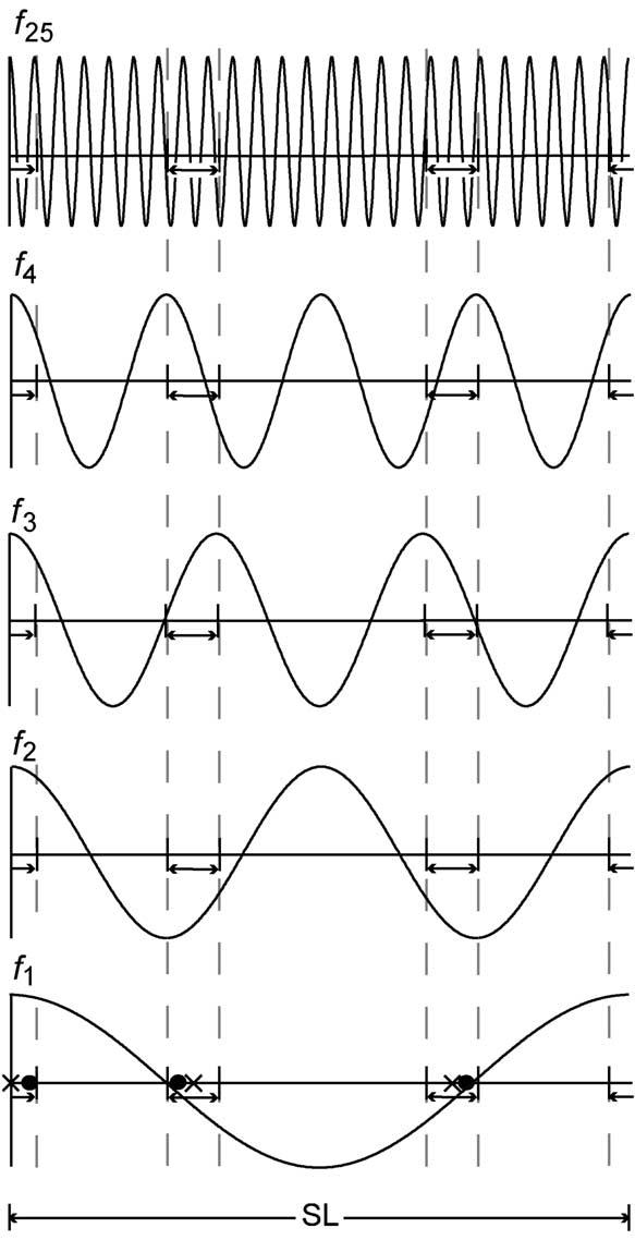
Diagram of how the jitter-limits on SL, expressed as time-domain limits, affect the range of cosine values that can be used in the Q-magnitude calculation, at higher Fourier frequencies. The baseline for f₁ is the same as the sequence shown in Fig. A1(A).

Fig. A3.

Diagram of how the jitter-limits and stimulation points on SL, expressed as angles in the frequency-domain, affect the ω_s values at different Fourier frequencies. The baseline for the lowest frequency (f₁) is the same as the circular sequence shown in Fig. A1(B). Note how these temporal limits occupy larger and larger percentages of the cycle length as frequency increases (in multiples of the primary frequency). Note also that with higher Fourier frequencies, due to the k multiplier, the angle of a given stimulus falls in different quadrants than its angle in SL, and at high-enough frequencies the angle exceeds 2π.

In Fig. A3 we diagram the same frequencies as in Fig. A2, but show only a single cycle of each. The inner circle of Fig. A3 is identical with Fig. A1(B), with the stimuli now numbered. Note in Fig. A3 how the jitter-limits increase with Fourier frequency as a percentage of the cycle. This is a direct consequence of the fact that k is a multiplier of the angles ω_s in Eq. (C4), and that f=k/SL. Thus, when the jitter-limits are expressed as angles, for a higher f_k the jitter-limit-angle has been multiplied by k. In Fig. A3 there are no jitter-limits shown for f₂₅ because the limit at that frequency is greater than 2π.

Using the mechanical analogy, one can now intuit the approximate Q-magnitudes at some frequencies. At f₁ the Q-magnitude must be near zero because the ω_s values are all close to those of a uniform sequence, as shown in Fig. A1(B). On the other hand, the Q-magnitude for f₃ must be close to 3 because all of the angles corresponding to the stimuli are within the same jitter-limits (near ω=0). The angles are grouped simply because the points on each circle are the product kω_s, and with 3 stimuli located close to periodicity in SL, the 3 products will be within the same region. However, the same logic does not apply to the grouping of the angles in f₂₅ near ω=π. At this higher frequency, the jitter-limits include the entire circle. But, because of the modulo nature of angles, the angle that results from kω_s is just the residue in the quotient (kω_s)/2π. The residue is not readily intuited, though the consequence for the Q-magnitude at f₂₅ is clearly near 3 (with a phase near π). Another approximate Q-magnitude that can be intuited from Fig. A3 is that for f₄. Note that the angles for stimuli 1 and 2 provide very little distance to the left of the ordinate, while the angle for stimulus 0 is far to the right. Thus, the Q-magnitude to balance such a system must be near unity, in the region of ω=0.

To understand the significance of Fig. A3, note that the vertical lines in Fig. A2 are a time-domain constraint, whereas the constraints on Q-magnitudes (e.g. greater than unity) are in the frequency-domain and are computed from the angles diagrammed in Fig. A3. The only way that the Q-magnitude at any given frequency f_k can be adjusted is by varying the stimulation-times on SL within the time-constraints on SL. But any adjustment of stimulation-times on SL will simultaneously affect the Q-magnitudes of all f_k in the passband frequencies.

For a complete mechanical analogy, one must visualize a set of disks, one disk for each Fourier frequency in the passband range. Each of the disks (frequencies) must have the same number of unit-weight balls as there are on SL, but the time-constraint jitter-range limits are at different angular positions for each disk (as is shown in Fig. A3). The angles of the stimulation points at any given f are the residue of integer multiples (by k) of the angles on SL, divided by 2π due to the modulo nature of sines and cosines. So, if a given higher frequency disk is too-well balanced (i.e. has a small, near-zero Q-magnitude), that disk can be unbalanced further (increasing the Q-magnitude) by moving the stimulation points on SL. However, this will also change the position of the balls on the other disks, so that the single set of stimulation points on SL must satisfy the frequency-domain requirements for every disk (frequency) in the passband range. Hopefully this demonstrates why it is difficult for the authors to visualize the process of finding good q-sequences.

The minimum time between D–A time-bins (Δ) determines the ‘smoothness’ of the SIs on the SL. When that smoothness is projected to the higher frequencies (by multiplication by k), then it can become ‘coarse’. For example, a change of position of a stimulation point of one Δ on the SL circle will be a change of 25Δ on the f₂₅ circle. Thus, if the Q-magnitude at f₂₅ is too small and one wants to alter the stimulation-sequence (on SL) to compensate, this may be difficult or impossible if Δ is large on SL, since some of the intermediate points on the f₂₅ circle that could provide the good Q-magnitude may not have corresponding points on SL. Hence, a high D–A rate can be useful in applying the QSD technique. It is noteworthy that this reason for a high D–A rate is unrelated to considerations based on stimulus frequency-content.

In summary, sequences are easier to find if:

1. The permitted jitter is made larger, since this allows for a greater opportunity to move stimulation points on SL so as to adjust the desired Q-magnitude at a variety of frequencies.

2. The number of stimuli per sequence is increased (assuming the same mean repetition-rate), which increases the length of the SL, with the following consequences:

   1. A greater number of balls on the circle means that the equilibrium balance equal in magnitude to the weight of a single ball $(\mathcal{Q}=1)$ can be found with less movement away from a uniformly spaced pattern. Hence, for the same Q-magnitude, the jitter can be less if the number of stimuli is greater. The number of stimuli per cycle is increased by increasing the SL, while keeping the mean repetition-rate about the same.
   2. The primary Fourier frequency is lower, which means that for a given passband frequency the Fourier integer (k) is larger, in which case the projection of the time-domain limits to that frequency are a larger percentage of the circle (see reason #1, and Figs. A2 and A3).

3. The digitizing rate for the timing-sequence is high enough so that a small change in position of a stimulation point on SL yields adequate control of the ω_s to give a Q-magnitude above unity. The digitizing rates for the timing-sequence, D–A conversion, and A–D conversion can be selected independently, based upon the requirements of each. However, if the equipment forces some of these rates to be identical, then there could be some situations where the rate for the timing-sequence predominates.

Appendix B. Alternative computational methods

QSD can be accomplished by a variety of computation techniques. By way of example, we describe 4 possible methods.

Appendix B.1. Method #1

This is the method described in the main part of this paper: QSD by transformation of $\tilde{v}\left(\theta \right)$ to the frequency-domain to form $\tilde{V}\left(f\right)$, and dividing by the union of $\tilde{\mathcal{Q}}\left(f^{\mathrm{P}}\right)$ and S(f^S) (Eq. (5)), followed by inverse Fourier transformation (IDFT) back to the time-domain to provide b̃(θ).

Technical notes:

1. The Fourier normalization factor ‘1/N’ is used in the IDFT.

2. The fast Fourier transform (FFT) is not specified because factors determining the length of SL generally do not permit the number of data points to be a power of 2. Padding with zeroes should not be used because this destroys the circularity of the vectors.

3. The use of the DFT is not a practical problem (despite being computationally slower than the FFT), because it is not necessary to compute those frequencies with stopband values near zero if the transition between passband and stopband is accomplished by steps which do not cause time-domain ringing.

Appendix B.2. Method #2

Estimation of b̃(θ) by a convolution calculation in the time-domain: $\tilde{v}\left(\theta \right)$ is convolved with a recovery-sequence r(θ), to yield b̃(θ):

$$\tilde{b}\left(\theta \right)=\tilde{v}\left(\theta \right)r\left(\theta \right)$$ (B1)

where © is circular convolution in the time-domain, and r(θ) is a convolution recovery sequence which is the union of $1∕\overleftrightarrow{\mathcal{Q}}\left(f^{\mathrm{P}}\right)$ and 1/S(f^S) transformed to the time-domain:

$$r\left(\theta \right)=\mathrm{IDFT}\left[\left\{\frac{1}{\overleftrightarrow{\mathcal{Q}}\left(f^{\mathrm{P}}\right)}\right\}\cup \left\{\frac{1}{S\left(f^{\mathrm{S}}\right)}\right\}\right]$$ (B2)

where IDFT is the inverse discrete fourier transform, which includes the Fourier 1/N factor.

Appendix B.3. Method #3

Estimation of b̃(θ) by time-domain circular cross-correlation. While this method is directly implied by Method #2, we include it here to resolve any nagging doubts that those familiar with the use of MLS in evoked-responses might have about whether QSD equations apply MLS. If an MLS is used as the timing-sequence, and one wished to find b̃(θ) by circular cross-correlation of a recovery sequence with the averaged data, the result will be the same as using the traditionally derived MLS recovery sequence, if this form of QSD is used:

$$\tilde{b}\left(\theta \right)=r_{\kappa }\left(\theta \right)\kappa \tilde{v}\left(\theta \right)$$ (B3)

where k represents circular cross-correlation in the time-domain and where the cross-correlation recovery-sequence, r_k(θ) is equal to r(−θ) from Eq. (B2), by definition.

Technical notes:

1. For Eq. (B3) to provide a b̃(θ) identical with that obtained by use of an MLS with an MLS-recovery-sequence, then r_k(θ) and r(−θ) must be identical to the MLS-recovery-sequence, r_MLS(θ). That this is true is proven in Appendix C.4.

2. The use of Methods #2 and #3 may be useful for online QSD computations, but the speed relative to Method #1 depends upon several factors: the size of the passband, the duration of SL, and the number of data-points in SL. In some cases Method #1 is actually computationally faster.

Appendix B.4. Method #4

Estimating b̃(θ) by forming a circulant convolution matrix utilizing q(θ), inverting the matrix, and multiplying by $\tilde{v}\left(\theta \right)$.

Technical notes:

1. In this computation all $\mathcal{Q}\left(f\right)$ are used, including those that are less than zero. So post-deconvolution filtering is likely to be necessary if the jitter is small. The filtering must be sufficient to deal with noise that has been amplified by a $\mid \mathcal{Q}\left(f^{\mathrm{S}}\right)\mid$ less than unity. Alternatively, the circulant matrix can be formed from r(t) (Eq. (B2)) so as to avoid deconvolution of such frequencies.

2. In our experience, neither the invertability nor the condition number of a matrix is sufficient to determine whether a sequence is acceptable. We point out that neither of these measures takes into account the effect the timing-sequence has on noise at specific frequencies. One group has used invertibility as a criterion for sequence selection (Delgado and Ozdamar, 2003).

Appendix C. Proofs and derivations

Appendix C.1. Proof that circular superposition is convolution

We now will show that the process of algebraically summing overlapped evoked-responses in circular vectors is mathematically equivalent to circular convolution, if q(θ)is binary. We first express the process of Fig. 3 mathematically

$$v\left(\theta \right)=\sum _{s=0}^{S-1}b(\theta -{\omega }_s)$$ (C1)

where:

• θ is an angle on the circular vector, in radians;

• ω_s is the angle (timing) of a given stimulus, s; stimuli are numbered sequentially from s=0 to S−1;

• S is the total number of stimuli.

In words, both Eq. (C1) and Fig. 3 show that at a given θ, v(θ) is the algebraic summation of all the b that overlap at that θ, the points of overlap being determined by the waveshape b(θ) and the timing locations ω_s.

Given Eq. (C1), and that q(ω_s)=1 for all s, the following equation is also true:

$$v\left(\theta \right)=\sum _{s=0}^{S-1}b(\theta -{\omega }_s)q\left({\omega }_s\right)$$ (C2)

If we define a new set of angles, ω_n, that includes every discrete angle in the circular vector, we can recast Eq. (C2) as a summation over all N of these angles in the circular vector, and obtain:

$$v\left(\theta \right)=\sum _{n=0}^{N-1}b(\theta -{\omega }_n)q\left({\omega }_n\right)\theta ={\omega }_0,{\omega }_1,{\omega }_2,\dots ,{\omega }_{N-1}$$ (C3)

where q(ω_n)=1 only for angles in the subset ω_s, while q(ω_n)=0 for all other angles. Eq. (C3) is the equation for the circular convolution of b(θ) with q(θ) in a commonly used form (Oppenheim et al., 1999; Poularikas, 1999), thus demonstrating that the process of Fig. 3 is convolution and that Eq. (1) correctly describes that process.

Appendix C.2. Derivation of $\mathcal{Q}$-magnitude

Appendix C.2.1. $\mathcal{Q}$-magnitude definition

The Q-magnitudes $(\mid \mathcal{Q}\left(f\right)\mid )$, which are the Fourier coefficients of the timing-sequence q(θ) are found by computing for each Fourier frequency, the square-root of the sum of the squared real and imaginary Fourier coefficients (Eq. (C4)):

$$\mid \mathcal{Q}\left(f_k\right)\mid =\sqrt{{\left[\sum _{s=0}^{S-1}\cos \left(k{\omega }_s\right)\right]}^2+{\left[\sum _{s=0}^{S-1}\sin \left(k{\omega }_s\right)\right]}^2}$$ (C4)

where:

• $\mid \mathcal{Q}\left(f\right)\mid$ is length of the vector sum of the real and imaginary Fourier components,

• f_k is a frequency which is an integer multiple of the primary Fourier frequency. In this paper (f) implies (f_k), k is an integer which indexes the discrete Fourier frequencies via the relationship f_k=k/SL,

• S is the total number of stimuli in the sequence-length, s is the sequential numbering of the stimuli in the sequence, and

• ω_s is the timing of the sth stimulus in the timing-sequence, taken as a fraction of the sequence-length, expressed as an angle, in radians.

In deriving Eq. (C4), we start with the equation for the discrete Fourier series, as presented in Oppenheim et al.'s (1999) textbook:

$$\mathcal{Q}\left(k\right)=\sum _{n=0}^{N-1}q\left({\omega }_n\right){\mathrm{e}}^{-j\frac{2\pi }{N}\mathit{nk}}$$ (C5)

where k is an index that takes on integer values, ω_n is the set of all discrete angles of the circular vector, and N is the number of data-points.

For didactic simplification, we will show the derivation of only the real part of the discrete complex Fourier coefficient. Noting that (2π/N)n is the expression for the N discretized angles of ω_n, we express the real part of Eq. (C5) as:

$$\mathrm{Re}\left[\mathcal{Q}\left(k\right)\right]=\sum _{n=0}^{N-1}q\left({\omega }_n\right)\cos \left(k{\omega }_n\right)$$ (C6)

We next change to ω_s in the cosine function, indexing on the sequential numbering of stimuli, s, whose total number is S. q(ω) is eliminated from the next equation since q(ω_n)=1 for the subset ω_s

$$\mathrm{Re}\left[\mathcal{Q}\left(k\right)\right]=\sum _{s=0}^{S-1}\cos \left(k{\omega }_s\right)$$ (C7)

Finally, we express the k of Q(k) as the kth harmonic of the primary Fourier frequency, where f_k can only take the values of k/SL, k being restricted to integers:

$$\mathrm{Re}\left[\mathcal{Q}\left(f_k\right)\right]\sum _{s=0}^{S-1}\cos \left(k{\omega }_s\right)$$ (C8)

This is the form of the real Fourier coefficient used in Eq. (C4).

Appendix C.3. Derivation that run-to-run differences are dominated by EEG ‘noise’

By definition, any voltage directly time-locked to the timing of the stimulus is ‘response’, while voltage from sources that are uncorrelated to the stimulus-timing are ‘noise’. The largest of the unwanted voltages is intermittent-motion artifact, and the second largest is the continuous EEG activity. For very small potentials, such as the ABR, the Johnson noise in the amplifier also may be larger than the signal. A problem in interpretation arises when the initial signal-to-noise ratio (SNR) is so poor that considerable averaging is necessary to detect the signal. Since averaging has changed the SNR, it seems logical that any variability of the signal waveform run-to-run must be due to differences in the signal, but this is not correct. Noise dominates run-to-run differences (after averaging), just as it dominated before averaging, as we will show.

The equations below relate to a single time-point in an average, so there are no (t) indices. At that averaged single time-point we have some numerical value, call it y. We will express the SNR of our single-time-point average as the ratio of the mean, $\overline{y}$ to the standard error of the mean, ${\sigma }_{\overline{y}}$:

$${\mathrm{SNR}}_{\text{average}}=\frac{\overline{y}}{{\sigma }_{\overline{y}}}$$ (C9)

The numerator of Eq. (C9) is not changed by N since as the summation of repeated y's occurs N times, the summation is divided by N to obtain $\overline{y}$. The effect of N (the number of times y is measured) on the SNR is entirely via the denominator of Eq. (C9), as shown by:

$${\sigma }_{\overline{y}}=\frac{{\sigma }_y}{\sqrt{N}}$$ (C10)

Looking at Eq. (C10), as N increases, the standard error $\sigma \overline{y}$ decreases, and it is this decrease that affects the SNR in Eq. (C9) because as ${\sigma }_{\overline{y}}$ gets smaller the SNR increases. However, in Eq. (C10), the numerator σ_y is unchanged by N. In words: The standard deviation of the data is not affected by N.

While we can calculate the standard deviation, σ_y, of the measurements that made up the average at the single time-point, we cannot separately measure the two components of σ_y that are of interest to us: (1) the standard deviation of the signal itself, and (2) the standard deviation of the noise (i.e. non-signal). But we can visualize these components, which, since they are independent, must be combined in quadrature to form the measured σ_y:

$${\sigma }_y=\sqrt{{\sigma }_S^2+{\sigma }_N^2}$$ (C11)

By inspection of Eq. (C11), and remembering that the square of the standard deviation (σ²) is called the ‘variance’, it can be seen that if the signal variance is much smaller than the noise variance, as it is in many evoked-response recordings, then the noise variance will predominate in σ_y, and in ${\sigma }_{\overline{y}}$ after averaging, as shown by substituting Eq. (C11) into Eq. (C10):

$${\sigma }_{\overline{y}}=\frac{{\sigma }_y}{\sqrt{N}}=\frac{\sqrt{{\sigma }_S^2+{\sigma }_N^2}}{\sqrt{N}}=\sqrt{\frac{{\sigma }_S^2+{\sigma }_N^2}{N}}$$ (C12)

Notice that averaging has no influence on the relationship between the signal and noise variances. Hence, run-to-run differences when all experimental conditions are held constant, are dominated by the residual noise (after averaging), and do not indicate how much the signal has varied between runs.

In this analysis, it is critical to distinguish between random changes and systematic changes in the signal. Clearly if there are systematic changes in the signal between runs, then those differences can be detected, even though signal variance, and even changes in signal variance, cannot be detected by run-to-run differences, in the presence of dominating random noise.

Appendix C.4. Proof that r_MLS(θ)=r(−θ)

We define r_MLS(θ) to be the recovery sequence used with MLS when scaled by the number of stimuli. The following equation can be derived from Burkard et al. (1990):

$$q_{\mathrm{MLS}}\left(\theta \right)r_{\mathrm{MLS}}(-\theta )=\delta \left(\theta \right)$$ (C13)

where © is circular convolution. From the relationship between convolution and cross-correlation we then have:

$$r_{\mathrm{MLS}}\left(\theta \right)\kappa q_{\mathrm{MLS}}\left(\theta \right)=\delta \left(\theta \right)$$ (C14)

where κ is circular cross-correlation. Taking Eq. (C14) to the frequency-domain:

$$R_{\mathrm{MLS}}^{\ast }\left(f\right)\mathcal{Q}\left(f\right)=1$$ (C15)

where * is the complex conjugate. It follows that:

$$R_{\mathrm{MLS}}\left(f\right)={\left(\frac{1}{\mathcal{Q}\left(f\right)}\right)}^{\ast }$$ (C16)

Since the IDFT of conjugate gives the time-reversed sequence, taking the IDFT of both sides of Eq. (C16) yields:

$$r_{\mathrm{MLS}}\left(\theta \right)=r(-\theta )$$ (C17)

which we set out to prove. Since, by definition, r_k(θ)=r(−θ) it follows that Eq. (B3) applies to MLS.

Appendix D. Terms and acronyms

Below are the acronyms and the terms used in this paper. If any of the time-domain functions below occur in the frequency-domain, then they are capitalized and shown with frequency as a variable.

b(θ)	the response, as would be recorded on a given data-recording channel in the absence of noise, to an individual stimulus in the sequence
b̃(θ)	the estimate of b(θ) from deconvolution of $\tilde{v}\left(\theta \right)$
©	time-domain circular convolution
Δ	the minimum time increment in a circular vector, which at its smallest is the period of the A–D, but which can be larger if adjacent data-points are ‘binned’ to increase the period; expressed as an angle in radians
duty cycle	the percentage time that a given device or process is ‘on’
e	a subscript indicating the experimental conditions under which data were obtained
fk	a frequency that is an integer multiple of the primary Fourier frequency; fk=k/SL
fP, fS	the frequencies in the passband, stopband
Fourier coefficient magnitude	the length of the vector sum of the real and imaginary Fourier components at a specified frequency in a Q-magnitude calculation (Eq. (C4))
k	an integer which, besides providing an index, also, in combination of with the inverse of the sequence-length, determines the multiples of the primary Fourier frequency that are computed as k is incremented by 1: fk=k/SL
IDFT	the inverse discrete fourier transform, which includes the 1/N normalization
κ	time-domain circular cross-correlation
n(θ)	additive, nonconvolved noise, not synchronized with the stimuli; instrumental noise, and noise from external sources are included in this term
ω	an angle used as an index in time-domain convolution
ωs	the angle in the circular vector q(θ) indicating the timing of the stimulus number s
Passband of the evoked-response	those frequencies necessary to display or use the estimated evoked-response waveform
$\mathcal{Q}\left(f\right)$	the real and imaginary Fourier coefficients at frequency f, as determined from q(θ) (the timing-sequence of the stimulation). These are the values by which the signal is convolved during recording, and is likely to have non-zero values at all f, including the stopbands
$\overleftrightarrow{\mathcal{Q}}\left(f\right)$	the Fourier coefficient values determined by the user for use in the deconvolution; usually equal to $\mathcal{Q}\left(f\right)$ in the passband unless there were ‘adjustments’. Usually not equal to $\mathcal{Q}\left(f\right)$ in the stopband
$\mid \mathcal{Q}\left(f\right)\mid$	the vector magnitude of the Fourier coefficients, at frequency f
$\left\{\mathcal{Q}\left(f\right)\right\}$	the set of $\mathcal{Q}\left(f\right)$ at all frequencies, or a subset of such frequencies
Q-magnitude	the vector magnitude of the Fourier coefficients of the timing-sequence
q-sequence	a sequence of ones and zeros in which the ones indicate timing for stimuli in which the intervals between ones are quasi-periodic. A q-sequence conforms to a rule set with both time-domain and frequency-domain constraints. A q-sequence generally has an SI-ratio less than unity and greater than zero
QSD	Q-sequence deconvolution
q(θ)	stimulus-sequence timing as determined by a circular q-sequence, expressed as an angle in the circular vector. A stimulus is generated at the time of each ‘1’ in the q-sequence
r(θ)	the recovery function, to recover b̃(θ) from time-domain convolution with $\tilde{v}\left(\theta \right)$
s	the index of a stimulus in a circular stimulation-sequence
S	the total number of stimuli in a circular stimulation-sequence
SI	stimulus interval, start-to-start. The SI should be distinguished from ISI, which is the inter-stimulus interval, end-to-start
SI ratio	(SImax–SImin)/(SImin)
SL	sequence length. Can also be considered to represent ‘sweep length’ (additionally means sensation level in ‘dBSL’)
Superposed	the process of combining additively by algebraic summation
Superposition	a linear process in which the voltage at a point resulting from several sources simultaneously active is the algebraic sum of the voltages that would result if each source were activated alone
θ	time in circular vectors, expressed as an angle in radians
v(θ)	the superposed waveforms of b(θ), when b(θ) is convolved with q(θ)
$\tilde{v}\left(\theta \right)$	v(θ) with added noise [n(θ)].
WAAD	wrap-around average deconvolution. This term was used in the initial poster and podium presentations of QSD. It was then realized that the average did not ‘wrap-around’, it was the response that wrapped. Thus, the term was not accurate. Further development of QSD showed that it did not have to be computed on an average if the signal-to-noise ratio was good. This was the final-straw that sunk the ‘WAAD’ terminology in a mixed metaphor. We apologize for any inconvenience caused by this acronym-lability

References

- Abd-al-Hady M, el-Mously M, Sallam F. Audiological findings following head trauma. J Laryngol Otol. 1990;104:927–36. doi: 10.1017/s0022215100114410. [DOI] [PubMed] [Google Scholar]
- Attias J, Pratt H. Auditory evoked potentials and audiological follow-up of subjects developing noise-induced permanent threshold shift. Audiology. 1984;23:498–508. doi: 10.3109/00206098409070089. [DOI] [PubMed] [Google Scholar]
- Burkard R, Hecox K. The effect of broadband noise on the human brainstem auditory evoked response. I. Rate and intensity effects. J Acoust Soc Am. 1983;74:1204–13. doi: 10.1121/1.390024. [DOI] [PubMed] [Google Scholar]
- Burkard R, Shi Y, Hecox KE. A comparison of maximum length and Legendre sequences for the derivation of brain-stem auditory-evoked responses at rapid rates of stimulation. J Acoust Soc Am. 1990;87:1656–64. doi: 10.1121/1.399413. [DOI] [PubMed] [Google Scholar]
- Chiappa K, Harrison J, Brooks E, Young R. Brainstem auditory evoked responses in 200 patients with multiple sclerosis. Ann Neurol. 1980;7:135–42. doi: 10.1002/ana.410070208. [DOI] [PubMed] [Google Scholar]
- Collette J, Antonelli A, Cesaro P, Degos J, Bellotto R, Felisati G, Peynegre R. Influence of stimulation frequency on the morphology of auditory evoked potentials in multiple sclerosis. Ann Otolaryngol Chir Cervicofac. 1984;101:631–5. [PubMed] [Google Scholar]
- Counter SA. Neurophysiological anomalies in brainstem responses of mercury-exposed children of Andean gold miners. J Occup Environ Med. 2003;45:87–95. doi: 10.1097/00043764-200301000-00017. [DOI] [PubMed] [Google Scholar]
- Daly D, Roeser R, Aung M. Early evoked potentials in patients with acoustic neuroma. Electroencephalogr Clin Neurolophysiol. 1977;43:151–9. doi: 10.1016/0013-4694(77)90123-7. [DOI] [PubMed] [Google Scholar]
- Debruyne F. Influence of age and hearing loss on the latency shifts of the auditory brainstem response as a result of increased stimulus rate. Audiology. 1986;25:101–6. doi: 10.3109/00206098609078375. [DOI] [PubMed] [Google Scholar]
- Delgado R, Ozdamar O. New methodology for acquisition of high stimulation rate evoked responses: continuous loop averaging deconvolution (CLAD) Assoc Res Otolaryngol, Abst. 2003:1650. [Google Scholar]
- Despland P, Galambos R. The auditory brainstem response (ABR) as a useful diagnostic tool in the intensive care nursery. Pediatr Res. 1980;14:154–63. doi: 10.1203/00006450-198002000-00018. [DOI] [PubMed] [Google Scholar]
- Don M, Allen A, Starr A. Effect of click rate on the latency of the auditory brain stem response in humans. Annals of Otology, Rhinology and Laryngology. 1977;86:186–95. doi: 10.1177/000348947708600209. [DOI] [PubMed] [Google Scholar]
- Elidan J, Collette J, Sohmer H, Gafni M, Kahana E. Contribution of changes in click rate and intensity on diagnosis of multiple sclerosis by brainstem auditory evoked potentials. Acta Neurol Scand. 1982;65(6):570–85. doi: 10.1111/j.1600-0404.1982.tb03111.x. [DOI] [PubMed] [Google Scholar]
- Eysholdt U, Schreiner C. Maximum length sequences—a fast method for measuring brain-stem-evoked responses. Audiology. 1982;21:242–50. doi: 10.3109/00206098209072742. [DOI] [PubMed] [Google Scholar]
- Frank Y, Vishnubhakat S, Pahwa S. Brain-stem auditory evoked-responses in infants and children with AIDS. Pediatr Neurol. 1992;8:262–6. doi: 10.1016/0887-8994(92)90362-3. [DOI] [PubMed] [Google Scholar]
- Fujikawa S, Weber B. Effects of increased stimulus rate on brainstem electric response (BER) audiometry as a function of age. J Am Audiol Soc. 1977;3:147–50. [PubMed] [Google Scholar]
- Fujita M, Hosoki M, Miyazaki M. Brainstem auditory evoked responses in spinocerebellar degeneration and Wilson disease. Ann Neurol. 1981;9:42–7. doi: 10.1002/ana.410090108. [DOI] [PubMed] [Google Scholar]
- Gerling I, Finitzo H. Auditory brainstem response with high stimulus rates in normal and patient populations. Ann Otol Rhinol Laryngol. 1983;92:119–23. doi: 10.1177/000348948309200204. [DOI] [PubMed] [Google Scholar]
- Harkins S, McEvoy T, Scott M. Effects of interstimulus interval on latency of the brainstem auditory evoked potential. Int J Neurosci. 1979;10:7–14. doi: 10.3109/00207457909160474. [DOI] [PubMed] [Google Scholar]
- Hecox K, Burkard R. Developmental dependencies of the human brainstem auditory evoked response. Ann N Y Acad Sci. 1982;388:538–56. doi: 10.1111/j.1749-6632.1982.tb50815.x. [DOI] [PubMed] [Google Scholar]
- Hecox K, Cone B, Blaw M. Brainstem auditory evoked response in the diagnosis of pediatric neurologic diseases. Neurology. 1981;31:832–40. doi: 10.1212/wnl.31.7.832. [DOI] [PubMed] [Google Scholar]
- Hyde M, Stephens S, Thornton A. Stimulus repetition rate and the early brainstem responses. Br J Audiol. 1976;10:41–50. [Google Scholar]
- Jacobson J, Murray T, Deppe U. The effects of ABR stimulus repetition rate in multiple sclerosis. Ear Hear. 1987;8(2):115–20. doi: 10.1097/00003446-198704000-00009. [DOI] [PubMed] [Google Scholar]
- Jerger J, Oliver T, Stach B. ABR testing strategies. In: Jacobson J, editor. The auditory brainstem response. College-Hill Press; San Diego, CA: 1985. [Google Scholar]
- Jewett DL. Volume conducted potentials in response to auditory stimuli as detected by averaging in the cat. Electroencephalogr Clin Neurophysiol. 1970;28:609–18. doi: 10.1016/0013-4694(70)90203-8. [DOI] [PubMed] [Google Scholar]
- Jewett DL. Functional blockade of impulse trains caused by acute nerve compression. In: Jewett D, McCarroll H, editors. Nerve repair and regeneration: its clinical and experimental basis. C.V. Mosby Co.; St. Louis: 1980. pp. 199–206. [Google Scholar]
- Jewett DL. Org Comput Neurosci. Chicago, IL: 2002. A novel technique for analysis of temporally-overlapped neural responses. [Google Scholar]
- Jewett DL, Williston J. Auditory evoked far fields averaged from the scalp of humans. Brain. 1971;94:681–96. doi: 10.1093/brain/94.4.681. [DOI] [PubMed] [Google Scholar]
- Jewett DL, Larson-Prior LJ, Baird W. A new technique for analysis of temporally-overlapped auditory-evoked responses. Assoc Res Otolaryngol, Abst. 2002:554. [Google Scholar]
- Jewett DL, Caplovitz G, Baird B, Larson-Prior L. Time-domain deconvolution of overlapped waveforms by Q-sequences. Assoc Res Otolaryngol, Abst. 2003:964. [Google Scholar]
- Jiang Z. Outcome of brain stem auditory electrophysiology in children who survive purulent meningitis. Ann Otol Rhinol Laryngol. 1999;108:429–34. doi: 10.1177/000348949910800502. [DOI] [PubMed] [Google Scholar]
- Jiang Z, Brosi D, Wilkinson A. Comparison of brainstem auditory evoked responses recorded at different presentation rates of clicks in term neonates after asphyxia. Acta Paediatr. 2001;90:1416–20. doi: 10.1080/08035250152708833. [DOI] [PubMed] [Google Scholar]
- Jiang Z, Brosi D, Wilkinson A. Auditory neural responses to click stimuli of different rates in the brainstem of very preterm babies at term. Pediatr Res. 2002;51:454–9. doi: 10.1203/00006450-200204000-00009. [DOI] [PubMed] [Google Scholar]
- Keith R, Jacobson J. MS and other demyelinating diseases. In: Jacobson J, editor. The auditory brainstem response. College-Hill Press; San Diego, CA: 1985. [Google Scholar]
- Kjaer M. Brain stem auditory and visual evoked potentials in multiple sclerosis. Acta Neurol Scand. 1980;62(1):14–19. doi: 10.1111/j.1600-0404.1980.tb02999.x. [DOI] [PubMed] [Google Scholar]
- Langner G. Periodicity coding in the auditory system. Hear Res. 1992;60:115–42. doi: 10.1016/0378-5955(92)90015-f. [DOI] [PubMed] [Google Scholar]
- Larson-Prior L, Hart MT, Jewett DL. Neural processing of high-rate auditory stimulation under conditions of various maskers. Neurocomputing. 2004;58–60:993–8.. [Google Scholar]
- Langner G. Neural processing and representation of periodicity pitch. Acta Otolaryngol Suppl (Stockholm) 1997;532:68–76. doi: 10.3109/00016489709126147. [DOI] [PubMed] [Google Scholar]
- Oppenheim A, Schafer R, Buck J. Discrete-time signal processing. Prentice-Hall; Upper Saddle River, NJ: 1999. [Google Scholar]
- Ozdamar O, Delgado R, Thombre K, Yavuz E, Anderson M. Acquisition of ABRs at very high stimulation rate using CLAD (continuous loop algorithm deconvolution) Assoc Res Otolaryngol, Abst. 2003:1675. [Google Scholar]
- Paludetti G, Maurizi M, Ottaviani F. Effects of stimulus repetition rate in the auditory brain stem responses (ABR) Am J Otol. 1983;4:226–34. [PubMed] [Google Scholar]
- Poularikas A. The handbook of formulas and tables for signal processing. CRC Press; Boca Raton, FL: 1999. [Google Scholar]
- Pratt H, Bleich N, Martin W. Three-channel lissajous' trajectory of human auditory brain-stem evoked potentials. III. Effects of click rate. Electroencephalogr Clin Neurophysiol. 1986;63:438–44. doi: 10.1016/0013-4694(86)90126-4. [DOI] [PubMed] [Google Scholar]
- Press W, Teukolsky S, Vetterling W, Flannery B. Numerical recipes in C: the art of scientific computing. Cambridge University Press; New York: 1992. [Google Scholar]
- Robinson K, Rudge P. The early components of auditory evoked potential in multiple sclerosis. In: Desmedt J, editor. Progress in clinical neurophysiology. Karger; Basel: 1977a. [Google Scholar]
- Robinson K, Rudge P. Abnormalities of the auditory evoked potentials on patients with multiple sclerosis. Brain. 1977;100:19–40. doi: 10.1093/brain/100.1.19. [DOI] [PubMed] [Google Scholar]
- Robinson K, Rudge P. The early components of auditory evoked potential in multiple sclerosis. In: Desmedt J, editor. Progress in clinical neurophysiology. Karger; Basel: 1977c. [Google Scholar]
- Shanon E, Gold S, Himmelfarb M. Assessment of functional integrity of brain stem auditory pathways by stimulus stress. Audiology. 1981;20:65–71. doi: 10.3109/00206098109072683. [DOI] [PubMed] [Google Scholar]
- Shi Y, Hecox K. Nonlinear system identification by m-pulse sequences: application to brainstem auditory evoked responses. IEEE Trans Biomed Eng. 1991;38:834–45. doi: 10.1109/10.83603. [DOI] [PubMed] [Google Scholar]
- Starr A, Brackmann D. Brain stem potentials evoked by electrical stimulation of the cochlea in human subjects. Ann Otol Rhinol Laryngol. 1979;88:550–6. doi: 10.1177/000348947908800419. [DOI] [PubMed] [Google Scholar]
- Stockard J, Rossiter V. Clinical and pathological correlates of brain stem auditory response abnormalities. Neurology. 1977;27:316–25. doi: 10.1212/wnl.27.4.316. [DOI] [PubMed] [Google Scholar]
- Stockard J, Sharbrough F. Detection and localization of occult lesions with brainstem auditory responses. Mayo Clin Proc. 1977;52:761–9. [PubMed] [Google Scholar]
- Stockard J, Stockard J, Sharbrough F. Nonpathologic factors influencing brainstem auditory evoked potentials. Am J EEG Technol. 1978;18:177–209. [Google Scholar]
- Stockard J, Stockard J, Sharbrough F. Brainstem auditory evoked potentials in neurology: methodology, interpretation, and clinical application. In: Aminoff M, editor. Electrodiagnosis in clinical neurology. Churchill Livingstone; New York: 1980. [Google Scholar]
- Stockard J, Stockard J, Coen R. Auditory brain stem response variability in infants. Ear Hear. 1983;4:11–23. doi: 10.1097/00003446-198301000-00005. [DOI] [PubMed] [Google Scholar]
- Tanaka H, Komatsuzaki A, Hentona H. Usefulness of auditory brainstem responses at high stimulus rates in the diagnosis of acoustic neuroma. J Otorhinolaryngol Relat Spec. 1996;58:224–8. doi: 10.1159/000276841. [DOI] [PubMed] [Google Scholar]
- Uri N, Schuchman G, Pratt H. Auditory brain-stem evoked potentials in Bell's Palsy. Arch Otolaryngol. 1984;110:301–4. doi: 10.1001/archotol.1984.00800310025005. [DOI] [PubMed] [Google Scholar]
- Van Olphen A, Rodenburg M, Verwey C. Influence of the stimulus rate of brain-stem-evoked responses in man. Audiology. 1979;18:388–94. doi: 10.3109/00206097909070064. [DOI] [PubMed] [Google Scholar]
- Weber B, Fujikawa S. Brainstem evoked response (BER) audiometry at various stimulus presentation rates. J Am Audiol Soc. 1977;3:59–62. [PubMed] [Google Scholar]
- Yagi T, Kaga K. The effect of the click repetition rate on the latency of the auditory evoked brain stem response and its clinical use for a neurological diagnosis. Arch Otorhinolaryngol. 1979;222:91–7. doi: 10.1007/BF00469746. [DOI] [PubMed] [Google Scholar]
- Zhang H, Wang W. Effect of hyperlipidemia on auditory brain stem responses (article in Chinese) Lin Chuang Er Bi Yan Hou Ke Za Zhi. 2002;16:19–20. [PubMed] [Google Scholar]
- Zollner C, Karnahl T, Stange G. Input–output function and adaptation behaviors of the five early potentials registered with the earlobe-vertex pick-up. Arch Otorhinolaryngol. 1976;212:23–33. doi: 10.1007/BF00456360. [DOI] [PubMed] [Google Scholar]