The Inconsistency of “Optimal” Cut-points Using Two ROC Based Criteria.

Abstract

The use of biomarkers is of ever increasing importance in clinical diagnosis of disease. In practice, a cut-point is required to dichotomize naturally continuous biomarker levels of individuals at risk for disease and those not. Two methods commonly used for establishing the “optimal” cut-point are the point on the ROC curve closest to (0,1) and the Youden index, J. Both have sound intuitive interpretations, the point closest to perfect differentiation and the point farthest from none, respectively, and are generalizable to weighted sensitivity and specificity. Under the same weighting of sensitivity and specificity, they identify the same cut-point as “optimal” in certain situations and different cut-points in others. In this paper, we examine the situations in which the two criteria agree or disagree and show that J is the only “optimal” cut point for given weighting with respect to overall misclassification rates. A data driven example is used to clarify and demonstrate the magnitude of the differences. We also demonstrate a slight alteration in the (0,1) criterion that retains its intuitive meaning, while resulting in consistent agreement with J. In conclusion, we urge that great care should be taken when establishing a biomarker cut-point for clinical use.

The proper diagnosis of disease and treatment administration is a task that requires a variety of tools. Through advancements in biology and laboratory methods a multitude of biomarkers are available as clinical tools for such diagnosis. These biomarkers are usually measured on some continuous scale with overlapping levels for diseased and non-diseased individuals. Cut-points dichotomize biomarker levels, providing benchmarks that label individuals as diseased or not based on “positive” or “negative” test results. Biomarker levels of individuals with known disease status are used to evaluate potential cut-point choices and hopefully identify a cut-point that is “optimal” under some criteria.

Such a dataset would be comprised of biomarker levels for individuals classified as coming from the diseased (D) or non-diseased $\text{(}\overline{\text{D}}\text{)}$ population. These levels could then be classified as a positive (+) or negative (−) test result based on whether the biomarker levels are above or below a given cut-point, respectively. In most instances, some individuals will be misclassified, thus truly belonging to a population other than the one indicated by their test results. The sensitivity (q(c)) and specificity (p(c)) of that biomarker for a given cut-point, c, are the probabilities of correctly identifying an individual’s disease status (i.e. true positives and true negatives)

$$q(c)=\text{Prob}(\text{test\hspace{0.17em}result}=+\hspace{0.17em}|\hspace{0.17em}\text{D})$$

$$p(c)=\text{Prob}(\text{test\hspace{0.17em}result}=-\hspace{0.17em}|\hspace{0.17em}\overline{\text{D}}\hspace{0.17em}).$$

Making 1 minus these values the probability of incorrect classification or false negatives (1 − q(c)) and false positives (1 − p(c)).

A receiver operating characteristic (ROC) curve is a mapping of this sensitivity by 1 minus specificity that has become a useful tool in comparing biomarker effectiveness (1–3). This comparison takes place through summary measures such as the area under the curve (AUC) and partial area under the curve (pAUC), with higher area values indicating higher levels of diagnostic ability (1, 2, 4). A biomarker with AUC=1 differentiates perfectly between diseased, sensitivity=1, and health, specificity=1, individuals. Meanwhile, an AUC=0.5 means that overall there is a 50:50 chance that the biomarker correctly identifies diseased or health individuals as such.

Though useful for biomarker evaluation, these measures do not inherently lead to benchmark “optimal” cut-points for clinicians and other healthcare professionals to differentiate between diseased and non-diseased individuals. Several methods have been proposed and applied to identify an “optimal” cut-point using sensitivity, specificity and the ROC curve (4–8). Confidence intervals and corrections for measurement error are some of the supporting statistical developments accompanying cut-point estimation (9). Applications of these techniques have been demonstrated in nuclear cardiology, epidemiology and genetics to mention some examples (7, 10, 11). In the Criterion section, we describe two criteria for locating this cut-point that have similar intuitive justification. In describing the mathematical mechanisms behind the criteria, we demonstrate that one of the criteria retains the intended meaning, while the other inherently depends on quantities that may differ from an investigators intention. The Example section demonstrates how the two criteria identify different cut-points for the classification of 120 preeclampsia cases and 120 controls based on plgf levels, biomarkers of angiogenesis, from nested case control study from the CPEP prospective cohort. Next, we discuss the appropriateness of the term “optimal” as it applies to each criteria. This is handled first with equally weighted sensitivity and specificity. Consideration of differing disease prevalence and costs due to misclassification are also presented as a practical generalization (5,12). We end with a brief discussion.

CRITERION

The closest to (0,1) criteria

If a biomarker perfectly differentiates individuals with disease from those without based on a single cut-point, q(c)=1 and p(c)=1, the ROC curve is a vertical line from (0,0) to (0,1) joined with a line from (0,1) to (1,1) with an AUC =1. However, for a less than perfect biomarker, q(c)<1 and/or p(c)<1, the ROC curve does not touch the (0,1) point. Here the choice of an “optimal” cut-point is less straight forward. A criteria has been suggested and utilized where the point on the curve closest to (0,1) is identified and the corresponding cut-point is labeled “optimal” (6, 7). The rational behind this approach is that the point on the curve closet to perfection, q(c)=1 and p(c)=1 should be the optimal cut point from all the available cut-point, thus intuitively minimizing misclassification. Mathematically, the point c* that satisfies the equation

$$\begin{array}{l}\text{min\hspace{0.17em}}\left\{\sqrt{{\text{(}1-q(c))}^2\hspace{0.17em}+\hspace{0.17em}{(1-p(c))}^2}\right\}\hspace{0.17em}\hspace{0.17em}\hspace{0.17em}\text{or}\\ \text{min\hspace{0.17em}}\left\{{\text{(}1-q(c))}^2\hspace{0.17em}+\hspace{0.17em}{(1-p(c))}^2\right\}\hspace{0.17em}\end{array}$$ (1)

fulfills this criteria and is thus labeled the cut-point that best differentiates between diseased and non-diseased.

This criterion can be viewed as searching for the shortest radii originating at the (0,1) point and terminating on the ROC curve. Reference arcs can be used to visually compare radial distances, with the arc corresponding to c* being tangent to the ROC curve and thus the minimum and interior of any of the concentric arcs possible. Figure 1 demonstrates this point where the dotted arc is completely interior, thus closer to (0,1), to the arc formed by the distance to an alternate point on the curve.

FIGURE 1.

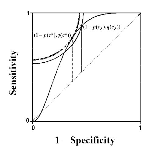
ROC curve based on simulated diseased and non-diseased populations. The vertical lines and reference arcs identify the Youden index, J, (solid) and the point closest to the (0,1) point (dotted) and their corresponding “optimal” cut-points c_J and c*, respectively.

The Youden Index

Another measure for evaluating biomarker effectiveness is the Youden index (J), first introduced to the medical literature by Youden (13). J is also a function of q(c) and p(c), such that

$$\begin{array}{c}J=max\{q(c)+p(c)-1\}\\ =\hspace{0.17em}max\{q(c)-(1-p(c))\}\end{array}$$ (2)

over all cut-points c, with c_J denoting the cut-point corresponding to J. On a ROC curve, J is the maximum vertical distance from the curve to the chance line or positive diagonal (figure 1), making c_J the “optimal” cut-point (5,14). The intuitive interpretation of the Youden index is that J is the point on the curve farthest from chance. It has also been defined as the accuracy of the test in clinical epidemiology (15).

Agreement/Disagreement

The criteria agree with respect to intuition; maximize and minimize the rate of individuals classified correctly and incorrectly, respectively. The question “Do they agree on the same “optimal” cut-point?”, now begs to be answered.

Suppose the biomarker of interest follows continuous distributions for both diseased and nondiseased populations that are known completely, leading to a true ROC curve. Our only distributional restriction is that a ROC curve is generated that is differentiable everywhere. This is intrinsic to the case where diseased and nondiseased individuals are assumed to follow any number of common continuous densities (i.e. normal, lognormal, gamma, ect.). Through differentiation, Appendix I shows that the two criteria only agree, c*= c_J = c, when q(c*) = p(c*) and q(c_J) = p(c_J). When either criteria identify a point on the curve such that q(c*) ≠ p(c*) or q(c_J) ≠ p(c_J), the criteria disagree on what cut-point is “optimal”, c* ≠ c_J.

An investigator with complete knowledge of a biomarker’s distributions could be faced with two different cut-points labeled “optimal” under the same intuition. Our motivation here is simply to show that they are different and address the appropriateness of the label “optimal” in a later section.

EXAMPLE

Preeclampsia affects about 5 percent of pregnancies, resulting in substantial maternal and neonatal morbidity and mortality (16). Although the cause remains unclear, the syndrome may be initiated by placental factors that enter the maternal circulation and cause endothelial dysfunction resulting in hypertension and proteinuria (16). Identifying women suffering from preeclampsia is a very important step in the management of the disease. Placenta growth factor (Plgf) is a promising biomarker for such classification with an AUC = 0.60 (95% CI 0.526–0.670); however at what level would a woman be classified as at risk for the disease. A nested case control study of 120 preeclampsia and 120 normal individuals were randomly chosen from the CPEP cohort study. Plgf levels were measured from serum specimens that were obtained before labor. The ROC curve in figure 2 was generated from the log transformed plgf levels. After calculating the distance to (0,1) and the distance to the diagonal for each point, the cut-points c*= 4.64 and c_J = 4.12 are identified, respectively. So, criteria with seemingly identical intuitive intent are close but disagree on an “optimal” cut-point. Again, here it is sufficient to demonstrate that disagreement exists. We will revisit this example after the question of “optimality” is addressed in the next section.

FIGURE 2.

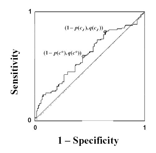
Empirical ROC curve using placenta growth factor (plgf) levels to differentiate between women diagnosed with preeclampsia and those without. The graph illustrates that the two points corresponding to cut-points labeled “optimal” by the point closest to (0,1), c*, and the Youden index, c_J, differ.

“Optimality”

When attempting to classify individuals based on biomarker levels, it is always the intent to do so “optimally”. However, the event of interest may intrinsically involve constraints which must for ethical or fiscal reasons be considered. These constraints are commonly accounting for the prevalence of the event in both populations and the costs of misclassification both monetary and physiological. So, now mathematic techniques of optimality must operate within these constraints but the idea of an “optimal” cut-point should remain; choosing a point which classifies the most number of individuals correctly and thus the least number incorrectly.

First let us assume the simplest scenario absent of constraints or weighting. By definition c_J found by equation 2 succeeds ideologically by maximizing the overall rate of individuals classified correctly, q(c_J) + p(c_J). As a result, the overall rate of misclassifications, (1 − q(c_J)) + (1 − p(c_J)), is minimized. So, we can say that c_J is “optimal” with respect to the total correct and incorrect classification rate and any cut-point that deviates from it is not.

Under the same scenario, the closest to (0,1) criteria in equation 1 minimizes the total squared misclassification rates, quadratic terms for which an ideology does not seem to exist other than being geometrically intuitive. Equation 1 can be expanded and rewritten as

$$\mathrm{min\hspace{0.17em}}\left\{(1-q(c))\hspace{0.17em}+\hspace{0.17em}(1-p(c))\hspace{0.17em}+\hspace{0.17em}(q{(c)}^2+p{(c)}^2)/2\right\}$$ (3)

to show that this criteria is minimizing the total of the misclassification rates and a third term, the average of squared correct classification rates. Unless a specific justification for this third term exists, its usage results in unwarranted and thus unnecessary misclassification because it identifies a point c* ≠ c_J.

Now, let us consider the circumstance where cost and prevalence are thought to be factors as they usually are in practice. Using decision theory, a generalized J can be formed where these factors are represented as a weighting of sensitivity and specificity. The function that minimizes expected loss in classifying a subject can be written as

$$\text{min\hspace{0.17em}}\left\{a\pi (1-q(c))\hspace{0.17em}+\hspace{0.17em}(1-\pi )(1-p(c))\right\}$$ (4)

where ‘a’ denotes the relative loss (cost) of a false negative as compared with a false positive and π is the proportion of diseased individuals in the population of interest (prevalence) (17, 18). It is easy to see that minimizing this expected loss over all possible threshold values is the same as

$$J=max\{q(c)+r*p(c)-1\}$$ (5)

where $r=\stackrel{(1-\pi )}{}/\underset{a\pi }{}.$ for r = 1 this is equivalent to J.

Weighting of the (0,1) criteria occurs similarly,

$$\mathrm{min\hspace{0.17em} }\{{(1-q(c))}^2+r*{(1-p(c))}^2\}$$ (6)

where r is exactly the same weighting estimate for cost and prevalence. The issue of the quadratic term remains

$$\mathrm{min\hspace{0.17em} }\{(1-q(c))+r*(1-p(c))\hspace{0.17em}+\hspace{0.17em}(q{(c)}^2+r*p{(c)}^2)/2\}$$ (7)

only now its weighted and unnecessary. Comparing this equation to equation 4 it is easy to see that this absolutely does not minimize loss due to classification.

Example Revisited

To demonstrate this unnecessary misclassification and its possible magnitude, we revisit the example of plgf levels used to identify preeclamptic women from those without the disease. Sensitivity and specificity at the cut-points previously identified are q(c*) = 0.592, p(c*) = 0.558 and q(c_J) = 0.817, p(c_J) = 0.358, respectively. The overall correct classification rate (q+p) is 1.150 for c* and 1.175 for c_J out of a possible 2, with a difference of 0.025. Without the justification for the third term in equation 3 and without weighting, this difference can be thought of as one person out of a hundred being unnecessarily misclassified. Relative cost and disease prevalence are often difficult to assess as discussed by Greiner et al (18). and the references cited therein. So we will not attempt to adjust in this example.

DISCUSSION

In this paper, we demonstrated the intuitive similarity of two criteria used to chose an “optimal” cutpoint. We then showed that the criteria agree in some instances and disagree in others. Plgf levels used to classify women as preeclaptic or not were used to demonstrate this point and quantify the extent of disagreement.

We addressed both criteria in the context of what an investigator might view as “optimal”, with and without attention given to misclassification cost and prevalence. Mathematically, J reflects the intention of maximizing overall correct classification rates and thus minimizing misclassification rates, while the choosing point closest to (0,1) involves a quadratic term for which the clinical meaning is unknown. It is for this reason that advacate for the use of J to find the “optimal” cutpoint.

Since, the (0,1) criteria is visually intuitive we have provided an amended (0,1) criteria in Appendix 2 that is likewise geometrically satisfying while consistently identifying the same “optimal” cut-point as J. This criteria relies on a ratio of radii originating at (0,1).

Additional motivation for using J is an ever increasing body of supporting literature. Topics such as confidence intervals and correcting the estimate for measurement error have been considered where the (0,1) citeria lacks such support.

Most importantly, cut-points chosen through less than “optimal” criteria or criteria that are “optimal” in some arbitrary sense can lead to unnecessary misclassifications, resulting in needlessly missed opportunities for disease diagnosis and intervention. We showed that J is “optimal” when equal weight is given to sensitivity and specificity, r = 1, and a generalized J is “optimal” when cost and prevalence lead to weighted sensitivity and specificity, r ≠ 1. So, when the point closest to (0,1) differs from the point resulting in J, using this criteria to establish a “optimal” cut-point does introduces an increased rate of misclassification, unnecessarily.

Appendix 1

For continuous ROC curves we make no distributional assumptions beyond that the probability density functions f_D and $f_{\overline{D}}$, for biomarker levels of diseased and non-diseased individuals respectively, form a ROC curve that is differentiable everywhere. This is the case when f_D and $f_{\overline{D}}$ are assumed to be any common continuous parametric distributions (i.e. normal, gamma, lognormal).

In order to locate these cut-points that minimize and maximize in equations 1 and 2, respectively, it is first necessary to locate critical values. So, differentiating equation 1,

$$\frac{\partial }{\partial c}\left[{(1-p(c))}^2+{(1-q(c))}^2\right]=2(1-p(c))\left(\frac{\partial (1-p(c))}{\partial c}\right)-2(1-q(c))\left(\frac{\partial q(c)}{\partial c}\right).$$ (A1.1)

Then set the derivative equal to zero,

$$\begin{array}{c}2(1-p(c*))\left(\frac{\partial (1-p(c*))}{\partial c}\right)-2(1-q(c*))\left(\frac{\partial q(c*)}{\partial c}\right)=0\\ (1-p(c*))\left(\frac{\partial (1-p(c*))}{\partial c}\right)=(1-q(c*))\left(\frac{\partial q(c*)}{\partial c}\right)\\ \frac{\partial q(c*)}{\partial (1-p(c*))}=\frac{1-p(c*)}{1-q(c*)}\end{array}$$ (A1.2)

Now, we differentiate the second criteria,

$$\frac{\partial }{\partial c}\left[q(c)-(1-p(c))\right]=\frac{\partial q(c)}{\partial c}-\frac{\partial (1-p(c))}{\partial c}$$ (A1.3)

and then setting equal to zero

$$\begin{array}{c}\frac{\partial q(c_J)}{\partial c}-\frac{\partial (1-p(c_J))}{\partial c}=0\\ \frac{\partial q(c_J)}{\partial c}=\frac{\partial (1-p(c_J))}{\partial c}\mathrm{\hspace{0.17em} }\\ \frac{\partial q(c_J)}{\partial (1-p(c_J))}=1\end{array}$$ (A1.4)

The forms of both A1.2 and 4 define the critical points of the criteria in equation 1 and 2, respectively, by the slopes of their corresponding points on the ROC curve. Since these solutions are not necessarily unique, multiple solutions may exist, i.e. local maximums or minimums. Therefore, all solutions and endpoints must be evaluated so that c* and c_J are global solutions.

Equations A1.2 and 4 show us that the (0,1) and J methods agree, c*= c_J = c, only when q(c*) = p(c*) and thus (1−p(c*))/(1−q(c*)) = 1. When q(c*) ≠ p(c*), the criteria disagree on what point is optimal, c* ≠ c_J. We will discuss which criteria might be “optimal” later, but for now our motivation is simply to show that they are different.

Appendix 2

Equation 1 identifies the point closest to perfection but irrespective of the possibilities of imperfection. In other words, this criterion minimizes the distance from (0,1) to the curve but fails to take into account the possible distance to the chance line or weighting the distances in equation 1. What if instead we minimize the proportion of the smaller radii (r₂) to the larger (r₁) displayed in figure 3 such that

FIGURE 3.

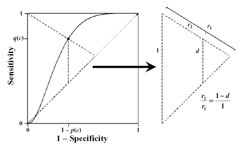
Similar triangles formed from a point on a ROC curve displaying that the ratio of radii extending from the (0,1) point, r₂ to r₁, is equal to one minus the height of the curve from the diagonal or chance line, d = q(c)−(1−p(c)).

$$\begin{array}{c}min\hspace{0.17em}\left\{\sqrt{\frac{r_2{}^2}{r_1{}^2}}\right\}=min\hspace{0.17em}\left\{\sqrt{\frac{{(1-p(c))}^2+{(1-q(c))}^2}{{\left(\frac{1-p(c)}{1-d}\right)}^2+{\left(1-\frac{1-p(c)}{1-d}\right)}^2}}\right\}.\\ =min\hspace{0.17em}\{1-d\}\end{array}$$ (A2.1)

where d = q(c) − (1 − p(c)), we obtain a weighted criterion.

The relation in equation A2.1 can be derived algebraically or by using proportionality of the triangles in figure 3 such that $\frac{r_2}{r_1}=\frac{r_1-(r_1-r_2)}{r_1}=1-\frac{(r_1-r_2)}{r_1}=1-\frac{d}{1}$. Figure 3 also, provides a visual reference for the proposed weighting, as radii passing through different points on the curve have different distances to the chance line but are treated uniformly in equation 1.

It is now easily seen that the differentiation

$$\begin{array}{r}\frac{\partial }{\partial c}\{1-d\}=-\frac{\partial q(c)}{\partial c}+\frac{\partial (1-p(c))}{\partial c}=0\\ \frac{\partial q(c)}{\partial (1-p(c))}=1\end{array}$$

leads to the same critical points on the ROC curve as J and thus to identical cut-points c* = c_J.

References

- 1.Zhou XH, Obuchowski NA, McClish DK. Statistical Methods in Diagnostic Medicine. New York: John Wiley & Sons, Inc., 2002.
- 2.Faraggi D. Adjusting ROC curves and realted indices for covariates. Journal of the Royal Statistical Society, Series D, The Statistician. 2003;52:179–192. [Google Scholar]
- 3.Schisterman EF, Faraggi D, Reiser B. Adjusting the generalized ROC curve for covariates. Statistics in Medicine. 2004;23:3319–3331. doi: 10.1002/sim.1908. [DOI] [PubMed] [Google Scholar]
- 4.Pepe M. The Statistical Evaluation of Medical Tests for Classification and Prediction. New York: Oxford University Press Inc., 2003.
- 5.Zwieg MH, Campbell G. Receiver-Operating Characteristic (ROC) Plots: A Fundamental Evaluation Tool in Clinical Medicine. Clinical Chemistry. 1993;39(4):561–577. [PubMed] [Google Scholar]
- 6.Coffin M, Sukhatme S. Receiver Operating Characteristic Studies and Measurement Errors. Biometrics. 1997;53:823–837. [PubMed] [Google Scholar]
- 7.Sharir T, Berman DS, Waechter PB, Areeda J, Kavanagh PB, Gerlach J, Kang X, Germano G. Quantitative Analysis of Regional Motion and Thickening by Gated Myocardial Perfusion SPECT: Normal Heterogeneity and Criteria for Abnormality. Journal of Nuclear Medicine. 2001;42:1630–1638. [PubMed] [Google Scholar]
- 8.van Belle G. Statistical Rules of Thumb. New York: John Wiley & Sons, Inc., 2002;98.
- 9.Perkins NJ, Schisterman EF. The Youden Index and the Optimal Cut-Point Corrected for Measurement Error. Biometrical Journal 2005; in press. [DOI] [PubMed]
- 10.Schisterman EF, Faraggi D, Brown R, Freudenheim J, Dorn J, Muti P, Armstrong D, Reiser R, Trevisan MJ. TBARS and cardiovascular disease in a population-based sample. Journal of Cardiovascular Risk. 2001;8:219–225. doi: 10.1177/174182670100800406. [DOI] [PubMed] [Google Scholar]
- 11.Chen R, Rabinovitch PS, Crispin DA, Emond MJ, Koprowicz KM, Bronner MP, Brentnall TA. DNA Fingerprinting Abnormalities Can Distinguish Ulcerative Colitis Patients with Dysplasia and Cancer from Those Who Are Dysplasia/Cancer-Free. American Journal of Pathology. 2003;16(2):665–672. doi: 10.1016/S0002-9440(10)63860-6. [DOI] [PMC free article] [PubMed] [Google Scholar]
- 12.Barkan N. Statistical Inference on r * Specificity + Sensitivity, Doctoral dissertation. University of Haifa, 2001 pp69–74.
- 13.Youden WJ. An index for rating diagnostic tests. Cancer. 1950;3:32–35. doi: 10.1002/1097-0142(1950)3:1<32::aid-cncr2820030106>3.0.co;2-3. [DOI] [PubMed] [Google Scholar]
- 14.Schisterman EF, Perkins NJ, Aiyi L, Bondell H. Optimal cut-point and its corresponding Youden Index to discriminate individuals using pooled blood samples. Epidemiology. 2005;16(1):73–81. doi: 10.1097/01.ede.0000147512.81966.ba. [DOI] [PubMed] [Google Scholar]
- 15.Chmura Kraemer, H. Evaluating Medical Tests: Objective and Quantitative Guidelines, 1992, SAGE, Newbury Park, California
- 16.Levine RJ, Maynard SE, Qian C, Lim KH, England LJ, Yu KF, Schisterman EF, Thadhani R, Sachs BP, Epstein FH, Sibai BM, Sukhatme VP, Karumanchi SA. Circulating angiogenic factors and the risk of preeclampsia. N Engl J Med. 2004;350(7):672–83. doi: 10.1056/NEJMoa031884. [DOI] [PubMed] [Google Scholar]
- 17.Geisser, S Comparing two tests used for diagnostic or screening processes. Statistics and Probability letters. 1998;40:113–119. [Google Scholar]
- 18.Greiner M, Pfeiffer D, Smith RM. Principles and Practical Application of the Receiver-operating Characteristic Analysis for Diagnostic Tests. Preventive Veterinary Medicine. 2000;45:23–41. doi: 10.1016/s0167-5877(00)00115-x. [DOI] [PubMed] [Google Scholar]