Selective Phenotyping for Increased Efficiency in Genetic Mapping Studies

Abstract

The power of a genetic mapping study depends on the heritability of the trait, the number of individuals included in the analysis, and the genetic dissimilarity among them. In experiments that involve microarrays or other complex physiological assays, phenotyping can be expensive and time-consuming and may impose limits on the sample size. A random selection of individuals may not provide sufficient power to detect linkage until a large sample size is reached. We present an algorithm for selecting a subset of individuals solely on the basis of genotype data that can achieve substantial improvements in sensitivity compared to a random sample of the same size. The selective phenotyping method involves preferentially selecting individuals to maximize their genotypic dissimilarity. Selective phenotyping is most effective when prior knowledge of genetic architecture allows us to focus on specific genetic regions. However, it can also provide modest improvements in efficiency when applied on a whole-genome basis. Importantly, selective phenotyping does not reduce the efficiency of mapping as compared to a random sample in regions that are not considered in the selection process. In contrast to selective genotyping, inferences based solely on a selectively phenotyped population of individuals are representative of the whole population. The substantial improvement introduced by selective phenotyping is particularly useful when phenotyping is difficult or costly and thus limits the sample size in a genetic mapping study.

GENETIC mapping involves the ascertainment of phenotype in a genetically segregating population followed by an analysis of association between the phenotype and genotypes at marker loci spanning the entire genome. Due to high-throughput technologies, genotyping no longer limits the sample size in a genetic mapping study. Increasingly, the cost and logistics of phenotyping impose limits on sample size. This is especially true of phenotypes involving complex physiological or behavioral traits.

Microarray technology has broadened our definition of phenotype to include the mRNA abundance data obtained from microarray experiments. Gene mapping using microarray data as phenotypes is now emerging (Brem et al. 2002; Schadt et al. 2003; Yvert et al. 2003) and will soon be commonplace (Jansen and Nap 2001; Doerge 2002; Bochner 2003). The high cost of microarrays greatly limits the sample size of a gene mapping study of mRNA abundance traits.

We have studied the inheritance of physiological traits and mRNA abundance traits in an F₂ sample segregating for obesity and diabetes (Stoehr et al. 2000; Lan et al. 2003). Because of the high cost of microarrays, we had a strong incentive to limit the number of animals studied with microarrays. Having a fairly large sample of animals that were genotyped, we asked if a selected subset of this full mapping panel would be more informative than a randomly selected subsample.

We describe a selective phenotyping strategy that can substantially increase detection efficiency whenever phenotyping requires much more effort than genotyping. We performed simulations to study the behavior of selective phenotyping and then successfully applied the method to our mouse gene expression mapping study.

We first consider the performance of selective phenotyping for a range of sizes of full mapping panels and for different proportions of individuals selected in subsamples from these mapping panels. We then show how sensitivity improves with increasing score, a measure of genetic difference, when some markers used for selective phenotyping are linked to QTL. Next, we investigate the relative merits of different criteria of selective phenotyping. Finally, we examine the performance of selective phenotyping on our mouse mapping panel.

MATERIALS AND METHODS

F₂ mice selection:

Our mapping panel includes 108 (B6 × BTBR) F₂-ob/ob mice used to study QTL associated with obesity and diabetes (Stoehr et al. 2000). The framework map was constructed with MapMaker/EXP (Lander et al. 1987) and consists of 188 microsatellite markers spanning the 19 mouse autosomes, composing a framework map with average spacing of 20 cM augmented by markers in identified regions. The phenotypes include 11 physiological traits, such as fasting plasma glucose, fasting plasma insulin, and body weight at 8 and 10 weeks of age, and the abundance of 12 mRNA species involved in liver metabolic pathways relevant to insulin action and glucose homeostasis, such as stearoyl-CoA desaturase 1 (SCD1), fatty acid synthase (FAS), and acyl-CoA oxidase (ACO). The liver mRNA abundances in the F₂ mice were estimated using the quantitative real-time reverse transcriptase-PCR (qRT-PCR) as described earlier (Lan et al. 2003). Previous studies have found that regions on chromosomes 2, 4, 5, 9, 16, and 19 harbor QTL for insulin, glucose, and SCD1 mRNA traits (Stoehr et al. 2000; Lan et al. 2003). In this study, we selected 60 mice according to their genotypes on these six chromosomal regions for subsequent analysis.

Selection criteria:

Assuming only a modest number of quantitative trait loci, how do we best select a subsample from the mapping panel for phenotyping? We want to select individuals that are genotypically dissimilar to maximize the available genetic information. Detection of a major QTL in an F₂ mapping panel with an additive genetic effect has the most power in a sample that has a 1:1 ratio of individuals homozygous for either parental genotype at the QTL locus (O'Bren and Funk 2003). A random sample at this locus would have an ∼1:2:1 ratio of A:H:B genotypes and would require up to twice the sample size for comparable power to detect a strictly additive effect. If we cannot afford to phenotype all individuals, we would prefer to selectively phenotype equal numbers of homozygotes. The selection criterion can also be modified to favor a 1:1:1 ratio to detect general differences among the three genotypes. Inference obtained through standard interval mapping is not affected by selection based on marker genotypes (see appendix). This is in contrast to selective genotyping where it is well known (Lander and Botstein 1989) that ignoring unselected progeny leads to bias in QTL effect estimation.

We build our algorithm on the experimental design concept of minimum moment aberration (MMA), which is equivalent to other statistically justified criteria (Xu 2003). The basic idea is to select a subsample of individuals that are as dissimilar as possible. MMA measures similarity for a subsample as an average of all pairwise similarities, K₁ (see appendix), with the similarity for two individuals being the “similarity” between their marker genotypes summed across a subset of markers from the linkage map. Similarity at a marker could be 1 for the same genotype and 0 for different genotype to emphasize general QTL effects. For a subsample of 60 individuals, we prefer to measure similarity as the number of alleles two individuals share (0, 1, or 2) to optimize detection of additive genetic effects. This measure preferentially selects homozygotes at the markers of interest.

The MMA criterion depends on the size of the mapping panel and the number of markers considered in the similarity measure. We standardized the similarity K₁ to allow comparison across experiments of different size. Our score is normalized between 0 and the square root of sample size,

where the “max” is the maximum possible value of K₁ and the “range” is the difference between the maximum and the minimum possible (see appendix). Note that because of the inverse relationship between K₁ and the score, minimizing similarity is equivalent to maximizing the score.

Our MMA criterion corresponds to the first moment or mean, K₁, and optimizes selection for nonepistatic effects. The second moment or variance, K₂ (see appendix), would further optimize for epistatic QTL. Xu (2003) recommends first selecting subsamples based on K₁ and then selecting the design with the smallest K₂. Alternatively, we could consider some weighted average of K₁ and K₂. Simulations (not shown) suggest little difference between these approaches in practice. Higher-order moments are probably not effective and are not considered further.

Two-step implementation:

Subset selection is a challenging computational problem due to many possible subsets to evaluate. Therefore, we propose a two-step approach: forward selection of individuals followed by optimization through pair swapping. Initially, the pair of individuals with the minimum similarity is selected. Each iteration adds one individual to the set based on the MMA criterion. It is well known that this approach may not reach the global optimum, since individuals chosen earlier may no longer be optimal in light of later choices. The optimization step swaps individuals out of the chosen set to be replaced by new individuals. A swap is retained if the resulting set has a lower similarity. This swapping procedure is repeated until no larger dissimilarity can be found.

Genomic information:

When we have little information about genetic architecture, we could select individuals on the basis of a framework map for the entire genome (genome-wide selective phenotyping). However, if previous studies suggest that certain genomic regions may be important, we can employ chromosome-wide selective phenotyping, which uses information only from chromosomes of particular interest, or marker-based selective phenotyping, concentrating on a few genetic markers in the genomic regions of interest.

Performance measures:

We used simulations to establish the performance characteristics of different selective phenotyping strategies. Selected sets of individuals were compared to random samples of the same size and to the full mapping panel to assess the overall efficiency of selection. Detection of a QTL is defined as a LOD exceeding the permutation-based threshold (Churchill and Doerge 1994) within a 40-cM window surrounding the true locus. The following performance measures were used in this study:

• Specificity: one minus the false-positive rate is the percentage of simulation runs for which no QTL were found over regions of the genome where no QTL were present.

• Sensitivity: the percentage of simulation runs in which all QTL present were detected.

• QTL effect bias: the difference between expected and true value of the QTL effect.

• QTL effect standard error: typical deviation of estimated QTL effect.

• QTL location estimates: s is the average absolute distance of detected LOD peak from the known underlying QTL; c is the frequency that the true position falls into the interval defined by LOD within 1.5 of the peak LOD.

Simulations:

We conducted simulations under a variety of situations that we expect to encounter in a genetic mapping experiment. For each situation, we simulated 100 replicate F₂ mapping panels on the basis of the Haldane mapping function with evenly spaced (10 cM) markers. Environmental noise was drawn from a standard normal distribution, with heritability (0.25–0.75) coming from additive genetic effects. Significance thresholds were calculated on the basis of 100 permutations per simulated mapping panel at significance level 0.05.

We first considered efficiency over a wide range of situations, with varying size of mapping panels (N = 50–200), sample sizes (n = 10–N), and proportion of individuals selected (10–90%). We considered one QTL on chromosome 1 with heritability h² = 0.25, 0.50, 0.75, on the basis of the range of heritability encountered in previous studies (Broman and Speed 2002; Yvert et al. 2003). We primarily considered marker-based selective phenotyping, except for the last set of simulations.

We then addressed our specific problem with 110 F₂ individuals, up to 20 chromosomes of length 70–100 cM, and one to three QTL. Markers were placed every 10 cM along chromosomes, similar to that in Cheung et al. (2003). For each simulated mapping panel, a subset of 60 individuals was selected either at random or by using one of the three selective phenotyping methods. The subsets were compared with each other and with the full mapping panel in terms of sensitivity, specificity, bias, and precision of inferring the correct QTL.

Software:

The selective phenotyping algorithm was implemented in R (www.r-project.org). Multidimensional scaling was performed using the R/mva package. QTL analysis was performed using standard interval mapping with the R/qtl package (Broman et al. 2003).

RESULTS

How many individuals do we need for selective phenotyping?

We simulated various mapping panel sizes while keeping the selected sample size fixed (n = 50, h² = 0.25) and limiting attention to one 100-cM chromosome with one QTL at 35 cM. When progeny are selected randomly, no improvement of sensitivity is observed with increasing mapping panel size (Figure 1a). In sharp contrast, selective phenotyping based on flanking markers (30 and 40 cM) was able to take advantage of the increasing mapping panel. Sensitivity increased with mapping panel size and with the proportion selected. It leveled off when the selected proportion reached 50% (Figure 1a). With higher heritability, the curve levels off below 50% (data not shown). Fixing the selected proportion at 50% (n = 0.5N, h² = 0.25), the sensitivity increased roughly linearly with mapping panel size (Figure 1b). The intercept decreases for selected markers further away from the QTL position.

Figure 1.—

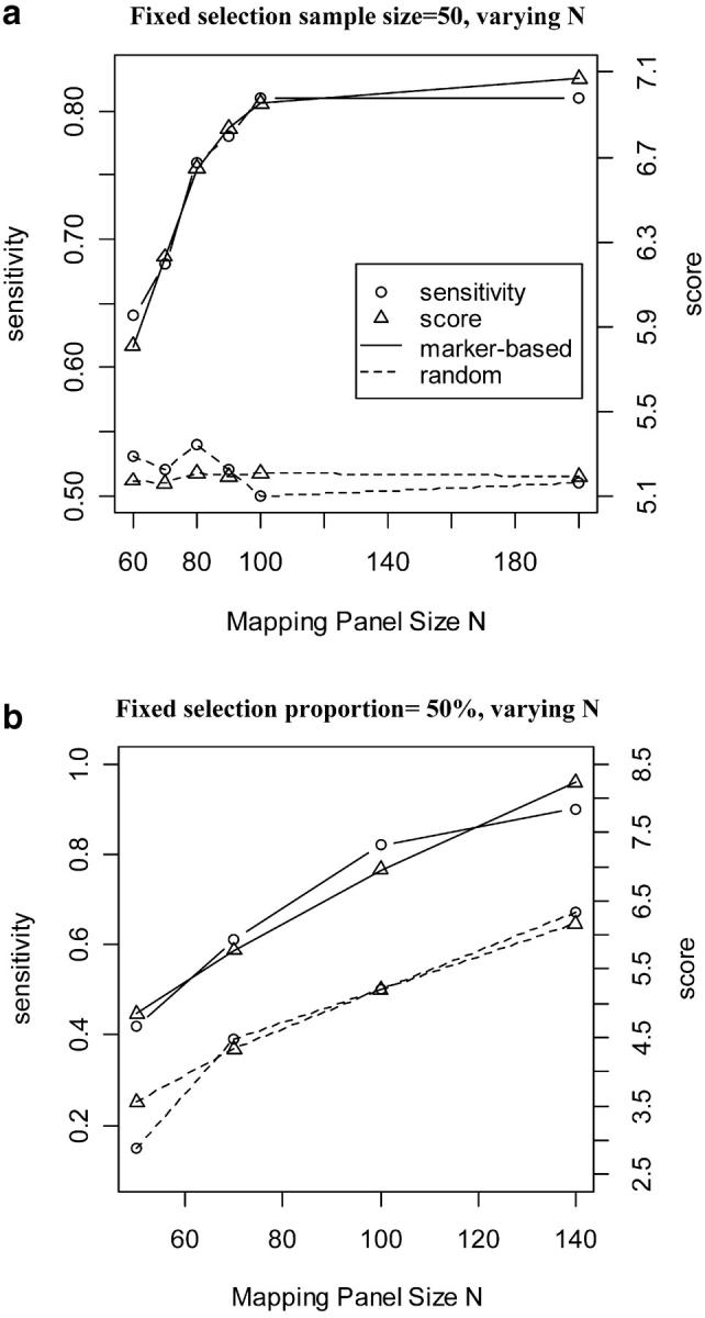
Effect of mapping panel size on sensitivity and score with selective phenotyping. F₂ progeny were selected on the basis of markers at 30 and 40 cM, from a mapping panel of varying size. The true QTL is located at 35 cM on a single-chromosome genome. The phenotype is simulated with heritability of 0.5. The horizontal axis represents the size of the mapping panel (N). (a) Effect of N on sensitivity (vertical axis on the left) and on score (vertical axis on the right), when 50 F₂ progeny were selected. (b) Effect of N on sensitivity (left) and score (right) when 50% of the panel was selected.

In a situation where the mapping panel is already established, what proportion of individuals do we need to selectively phenotype to retain high performance? For fixed mapping panel size (N = 100), as we increased the proportion selected, the sensitivity rose to a point of diminishing returns, depending on heritability (Figure 2a). Selection was more effective for highly heritable traits. Even with h² = 0.25, there is not much improvement with >50% selected. This is consistent with the findings with fixed selection sample size above. This indicates that, with high heritability, selectively phenotyping 50% of the progeny from the full mapping panel can retain most of the information needed for QTL detection. More progeny are needed when the heritability is low.

Figure 2.—

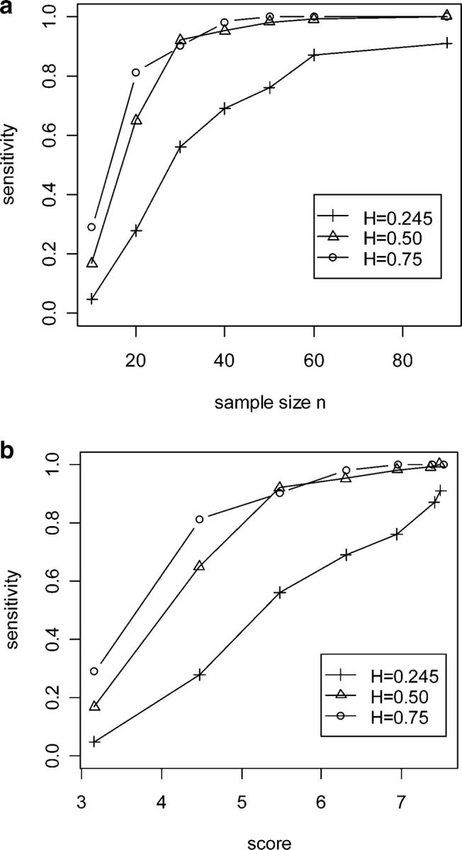
Effect of heritability and sample size on sensitivity and score with selective phenotyping. Varying numbers of progeny were selected on the basis of a marker at 30 cM, from a mapping panel of size 100. The true QTL is located at 33 cM on a single-chromosome genome. The phenotype is generated with heritability (H) of 0.245, 0.5, or 0.75. (a) The effect of sample size n (horizontal axis) on sensitivity (vertical axis) under different heritabilities. (b) The relationship between score (horizontal axis) and sensitivity (vertical axis) under different heritabilities.

These same relationships are reflected in curves with our genetic difference score (Figures 1b and 2b, averaged over 100 replicates). A major assumption behind the concept of selective phenotyping is that sensitivity is positively correlated with genetic difference. This assumption seems to hold, since for any fixed heritability, score appears to increase when sensitivity improves (Figure 2b) when some markers used for selective phenotyping are linked to QTL. Consequently, score is especially useful in “predicting” the performance of different selection schemes (not just selective phenotyping) without the need to refer to a particular phenotype or heritability.

What is the most appropriate selective phenotyping criterion?

We compared three selective phenotyping criteria that focus on different amounts of the genome. The genome-based criterion used markers across the entire genome region. The chromosome-based criterion used only markers on the chromosome that contained a known QTL, while the marker-based criterion had a single marker near the true QTL. A set of simulations had one QTL with pure additive effect (h² = 0.245) on chromosome 1 at 33 cM in a genome with 20 chromosomes. The mapping panel had 110 individuals, and 60 were selected by one of the criteria or by random sampling.

We found substantial differences in sensitivity to detect QTL when searching the whole genome (Figure 3). The sensitivity to detect a single QTL decreased as the number of chromosomes increased, regardless of selection criteria. With 20 chromosomes in the genome, gene mapping based on random sampling can detect QTL only 30% of the time, compared with 80% sensitivity of the full mapping panel. This tremendous loss of sensitivity can be rescued with selective phenotyping. Marker-based selection captured most (>70%) of the sensitivity of the full mapping panel, two- to threefold of the sensitivity obtained through random sampling. Genome-based (40%) and chromosome-based (>60%) selection were also considerably better than random selection. A restricted search of a portion of the genome yields smaller differences and higher sensitivity (Figure 3b). The dissimilarity scores for either the marker-based or chromosome-based criterion did not change with a restricted search of the genome (Figure 3a), as they depend only on markers used for selection, not on the QTL search strategy. However, the dissimilarity score for the genome-based criterion decreased as the region increased. The score is most useful for relative comparisons of the various selection methods when the search region is fixed.

Figure 3.—

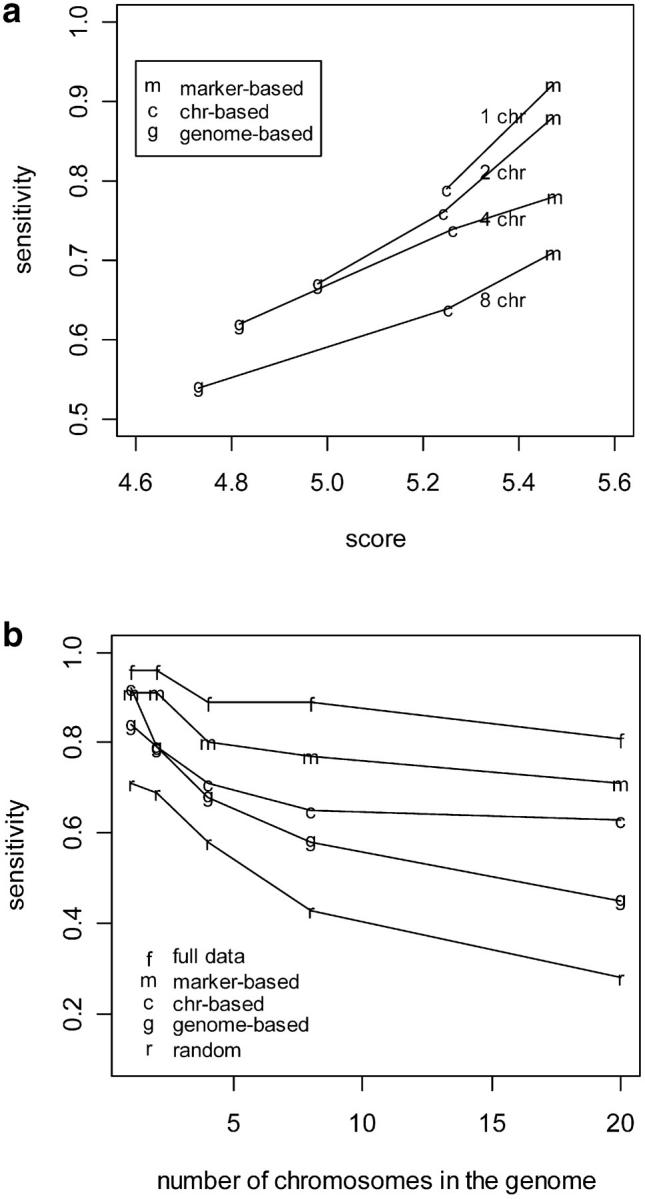
Comparison of selective phenotyping with random sampling. (a) The relationship between score (horizontal axis) and sensitivity (vertical axis) for different selective phenotyping methods with one, two, four, or eight chromosomes in the genome. “g” stands for genome-based, “c” for chromosome-based, and “m” for marker-based selective phenotyping methods. Sample size n is 30, mapping panel size is 100, and heritability is 0.5. (b) Sensitivity (vertical axis) comparison of genome-based (g), chromosome 1-based (c), and marker-based (m) selective phenotyping methods against full mapping panel analysis (f) and random selection (r). The horizontal axis denotes the number of chromosomes in the genome. Sixty F₂ progeny were selected from a mapping panel of size 110. The true QTL is located at 33 cM on chromosome 1 of a two-chromosome genome. Heritability is 0.245.

Figure 4a shows the median LOD maps of 100 replicates based on one QTL and a genome consisting of 10 chromosomes. The median LOD may not correspond to a result of any single analysis across the genome, but it provides a pointwise summary of LOD analysis for QTL. The full mapping panel had the highest LODs at the true QTL location, followed by the marker-based and chromosome-based methods. Genome-based selective phenotyping and random sampling had considerably lower LODs. Thus, the more specific we can be in selection using previous knowledge, the more sensitive our QTL analysis will be. Even without any prior information, our analysis still does slightly better than random sampling.

Figure 4.—

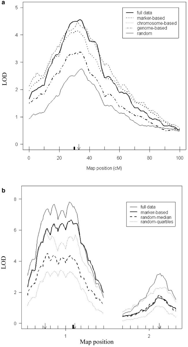
LOD map comparison for different selective phenotyping methods. (a) We simulated 100 F₂ mapping panels with 110 individuals, 10 chromosomes, and one QTL and performed standard interval mapping. Sixty individuals are selected using the three selective phenotyping methods: genome based (dotted dashed line), chromosome based (dotted line), and marker based (dashed line). Random method (thin solid line) and full mapping panel analyses (thick solid line) are provided as reference. The vertical axis is the median LOD obtained at each location. The horizontal axis represents the map location. The arrow points at the QTL location, and the solid bar points at the marker used for marker-based selection. (b) Marker-based selective phenotyping. We simulated 100 F₂ mapping panels with 110 individuals, markers every 10 cM, two linked QTL on one chromosome, and a third QTL on a second chromosome. For each simulated panel, we performed standard interval mapping. The vertical axis is the median or quartile LOD obtained at each position. The horizontal axis represents the map location for the two chromosomes. Arrows point to the QTL loci, vertical lines indicate markers, and the solid bar indicates the marker used for marker-based selection. Sixty individuals are selected randomly (dashed line) or using the marker-based selection (thick solid line). The 25 and 75% LOD quartile from random method (dotted line) and the median LOD from full mapping panel analyses (thin solid line) are provided as reference.

Genome-based selective phenotyping improves on random sampling when there is no prior information about genomic regions of interest for QTL. In a simulation with one additive QTL focusing on two chromosomes, the LOD curve for the genome-based selective phenotyping came close to the 75th percentile of the random method (not shown). No QTL signal was found on chromosome 2 for the full mapping panel or any subset; thus the false-positive rate is low. Both random selection and genome-based selective phenotyping maintained a specificity of at least 90%, lower than that of the full mapping panel (97%). Reducing the number of subjects selected seemed to affect detection power. Genome-based selective phenotyping had smaller bias and standard deviation for additive effect (Table 1). Our selection procedure tends to choose homozygous progeny more often, as expected, slightly favoring estimates of additive effects over dominance effects. A second simulation with one QTL having pure dominance showed that genome-based selective phenotyping still generated a higher LOD score than the random method, again tracking the 75th percentile of the random sampling (not shown). Other measures of performance did not change much. This supports using selective phenotyping even in the presence of full dominance.

TABLE 1.

Comparison of performance measures

	Full mapping panel	Random subset	Selective phenotyping
a. Genome-based selective phenotyping (60 mice) with one additive QTL and two chromosomes
Sensitivity (%)	97	69	77
Specificity (%)	97	92	91
LOD
33 cM	5.34 (0.21)	3.21 (0.16)	3.97 (0.17)
Region	5.59 (0.21)	3.48 (0.17)	4.24 (0.17)
Position
c (%)	99	94	94
s (cM)	4.24 (0.41)	8.34 (1.20)	8.24 (1.13)
Additive effects
Bias	0.021	0.055	0.010
SD	0.014	0.020	0.017
Dominance effects
Bias	−0.001	−0.0005	−0.005
SD	0.020	0.033	0.044
Variation
Bias	0.003	0.003	−0.007
SD	0.010	0.011	0.010
b. Simulated data with full dominance (full mapping panel analysis; 110 mice) and random selection (60 mice)
Sensitivity (%)	82	50	65
Specificity (%)	92	94	93
Additive effects
Bias	−0.006	−0.004	0.026
SD	0.017	0.024	0.018
Dominance effects
Bias	0.013	0.014	0.040
SD	0.022	0.036	0.040

Values in parentheses are standard errors.

Frequently, some chromosomes are of more interest at the beginning of a study. Suppose there is only one QTL, located on chromosome 1. Chromosome-based selective phenotyping based only on chromosome 1 provides considerably higher sensitivity than random sampling and slightly better sensitivity than genome-based selective genotyping (Figure 3). If we know further the approximate region(s) containing QTL of interest, then marker-based selective phenotyping, relying on one or a few markers, does even better (Figure 3). Thus, we can improve over random sampling provided the selection region is chosen correctly. However, if we choose regions for either criterion that do not contain QTL, such as chromosome 2, then selective phenotyping behaves like random selection on average for detection of QTL (not shown).

We performed another F₂ simulation with two QTL on chromosome 1 (at 23 and 62 cM) and one QTL on chromosome 2 (at 48 cM), all additive of the same magnitude of 0.7, and the residual phenotypic variation is assumed to be normally distributed with mean 0 and variance 1. Marker-based selective phenotyping with one marker near the first QTL on chromosome 1 had a higher LOD score and better detection for both QTL on chromosome 1 (Figure 4b). Sensitivity for the QTL on chromosome 2 is close to that of random sampling on average. Thus, the stronger and more specific the prior knowledge, the more detection power we can gain near these locations.

Mouse experimental design:

We have 108 (B6 × BTBR) F₂-ob/ob mice, and our goal is to select a subset of 60 mice for future gene expression studies. We chose them using the marker-based selective phenotyping approach with the following considerations: (1) the sensitivity gain with all 19 chromosomes would be minimal with genome-based selection methods; (2) we have previously identified six regions of particular interest, each ∼20 cM in length; and (3) there are few missing genotypes for the markers in these regions.

According to the specified criteria, the selected subjects should be as dissimilar as possible. To visualize the dissimilarity, we used multidimensional scaling (MDS), which projects individuals onto a two-dimensional map on the basis of their pairwise similarity. Selective phenotyping should choose individuals that are as dissimilar as possible, and we should not see any evidence of clumping. For the 108 mice, a two-dimensional projection explains >30% of the variation and shows no obvious pattern (Figure 5a), except that the progenies not selected tend to have more heterozygous genotypes in these six regions, which is desirable for our purpose.

Figure 5.—

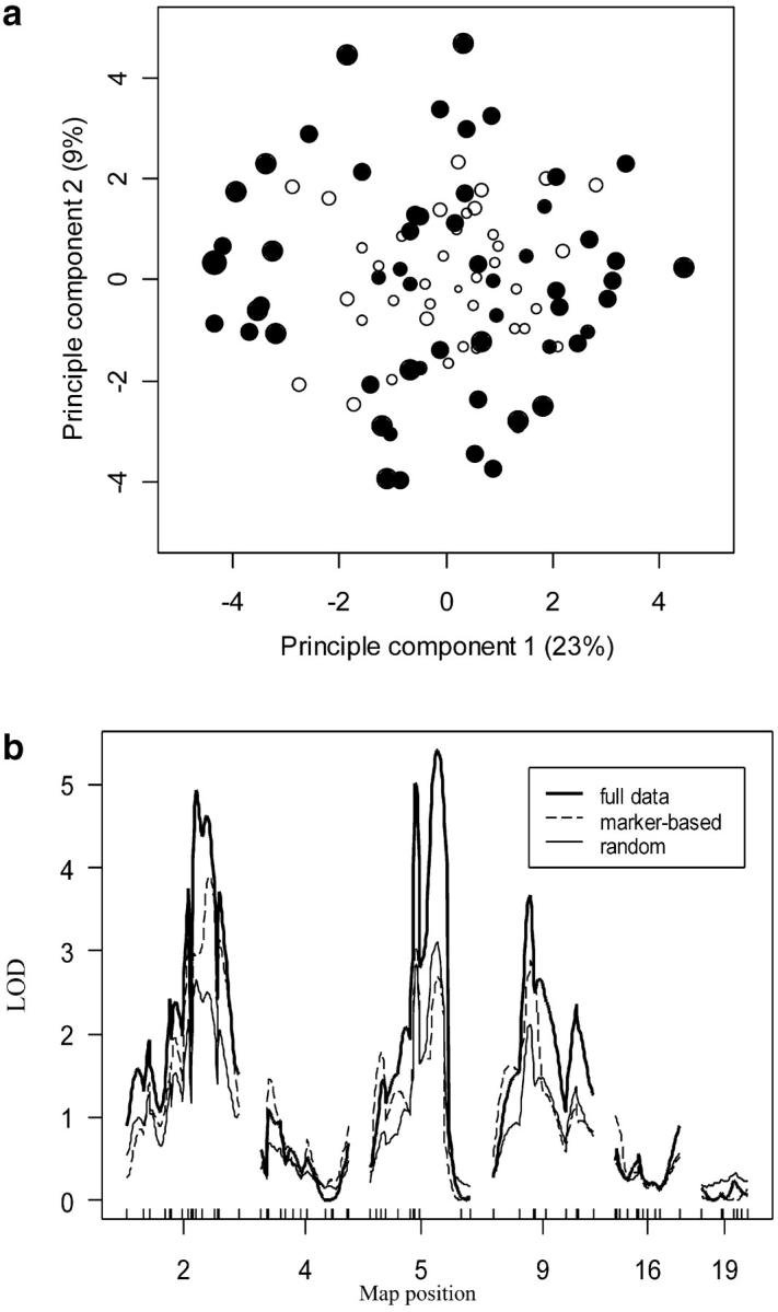
Mice selection experiment. (a) Multidimensional scaling visualization of the mice selection projected onto the first two principle components, which explain, respectively, 23 and 9% of the total variation. The 60 marker-selected mice are solid circles; the remaining 50 mice are open circles. The size of the circle measures the abundance of homozygous genotypes. The smaller the size, the more “H” it has. (b) Interval mapping of SCD1 trait for chromosomes 2, 4, 5, 9, 16, and 19. The LOD curves are for the full mapping panel with 110 (B6 × BTBR) F₂-ob/ob mice (thick solid line), 60 marker-selected mice (dashed line), and 60 randomly selected mice (thin solid line). The vertical axis is the LOD obtained at each position. The horizontal axis shows the chromosomes of interest with markers from the genetic map.

We examined the performance of our selective phenotyping method on the SCD1 phenotype by comparing its resulting LOD profile to that obtained through repeatedly drawing random samples of 60 mice (Figure 5b). Our LOD score was generally higher than the median LOD from random sampling with the exception of chromosome 5, where there appeared to be evidence for dominance and unequal variance for SCD1 across the marker genotypes. Selective phenotyping thus is superior to a random sample of equal size because it provides considerably more resolving power.

DISCUSSION

In this study, we present a criterion for selecting a subset of individuals for phenotyping based on their genotypes. We used an F₂ mapping panel for all the examples, but the method can be easily extended to other experimental designs and combined crosses. The decision to use genome-based, chromosome-based, or marker-based selection is made according to prior knowledge of both the presence and the localization of putative QTL. Stronger, more specific, and more accurate prior information leads to better resolution for those regions of interest. Chromosomes not used in the selection criterion tend to perform like a randomly chosen subset. By selecting individuals that are as genetically dissimilar as possible, the approach proposed here selects subsets of individuals that provide a better mapping panel than random sampling.

The choice of pairwise similarity depends on the research focus. Assigning the same pairwise similarity between different genotypes results in a balanced design, where approximately the same number of progeny is selected for each genotype. This is more desirable if we are equally interested in a broad range of hypotheses about gene action. For an F₂ single-QTL analysis, this includes tests for additivity, dominance, fully dominant and fully recessive. Further selection of individuals with identical K₁ based on smallest second-moment similarity, K₂, results in a more balanced design across pairs of markers, which can improve detection of epistasis. Alternatively, with a limited number of progeny, to reach sufficient detection power, one may want to focus on certain tests of interest. Additive effects are usually considered the most important and most prevailing among all. The similarity measure we present emphasizes the examination of additivity both within and across loci. There is little evidence from our simulations to suggest an improvement in performance when the second moment is included with our measure (not shown), but we have not carried out an in-depth study of epistatic QTL.

The MMA criterion is conceptually simple and easy to implement, but current theory relies on complete data and uncorrelated factors. Correlation from genetic linkage can be minimized by selecting widely spaced markers, in the extreme at most one per region. Since we had few missing genotypes in regions of interest, we imputed missing values on the basis of flanking markers using the Haldane map function of no interference. Repeated imputation yielded only minor changes in selection. More imputation error will generally be introduced into selective phenotyping when using chromosome-based or genome-based selection. We are investigating the importance of missing values and linkage in the experimental design criteria. A natural solution is to define similarity as the expected value of similarity measures based on the flanking marker genotypes when the genotype at this locus is missing.

Interval mapping may give biased estimates for QTL effects in the presence of selective genotyping (Lander and Botstein 1989). We demonstrate that interval mapping is robust against selective phenotyping. Therefore, the inference obtained through analyzing only the selected subjects is representative of the whole population. However, if segregation distortion is present in markers that are used (or not used) for selection, then the mapping panel may be associated with some unobserved selection. Selective phenotyping based on these markers cannot solve this intrinsic problem, but it will also not introduce another layer of bias.

We demonstrate in this article that genome-wide selective phenotyping has improved power on average over that of random sampling and can protect against the occasional (but undetectable) samples that have very low power. In a large experiment, a two-stage selective phenotyping could dramatically reduce cost and increase power. A first stage of genome-wide selection could identify promising genomic regions, which are then used for marker-based selective phenotyping. This is especially useful when more information about genetic architecture is expected to surface at a later stage of the study. Our focus on additive effects was dictated by being able to phenotype only 60 mice. A larger study with hundreds of individuals selected would naturally want to examine general effects. Results here point to the power of such a procedure.

The proposed selective phenotyping methods can be directly applied to many experimental designs. For more general population structure, especially in human genetics, major adjustment is needed. The possible number of genotypes at a certain locus may vary greatly, and the study subjects may come from an unknown number of hidden populations. The genetic similarity between each pair of subjects may be obtained through a more sophisticated alternative, relationship estimation (Goring and Ott 1997; McPeek and Sun 2000). However, situations may exist when it is desirable to retain subjects with a certain marker genotype pattern. Selective phenotyping can be performed after estimation of hidden populations (Corander et al. 2003) based on different genotype patterns. The genetic similarity measure shall be defined accordingly to reflect the population structure. It is worth mentioning that maximizing unrelatedness in a general population sample may lead to maximizing genetic heterogeneity in the sample, which may not be desirable in some cases.

We have demonstrated that selective phenotyping provides an effective strategy to maximize the efficiency of genetic mapping studies that require expensive or time-consuming assays. This can substantially reduce research costs while maintaining high power to detect QTL. This methodology could be extended to association studies to select individuals on the basis of haplotype block information.

APPENDIX

No bias for selective phenotyping:

It is well known that interval mapping is affected by selective genotyping based on phenotype information (Lander and Botstein 1989). However, inference obtained through standard interval mapping is not affected by selection based only on marker genotypes (Jin et al. 2003). To demonstrate this, we introduce a sampling variable, s_i, which equals 1 if the ith progeny is selected, 0 otherwise, with i = 1, … , N. Let Z_i and M_i denote the phenotype and flanking marker genotypes, respectively. Consider analyzing only the selected individuals (s_i = 1). Interval mapping (Lander and Botstein 1989) yields parameter estimators that model Pr(Z_i|M_i, s_i = 1). Note that sampling depends only on the marker genotypes: Pr(s_i = 1|z_i, M_i) = Pr(s_i = 1|M_i). It follows that

Thus inferences based on a model for Pr(z_i|M_i, s_i = 1) are directly interpretable in the model for Pr(z_i|M_i).

MMA similarity:

The first moment K₁ averages the similarity δ_ij between the ith and jth individuals (δ_ij = sum of number of alleles in common over all markers considered) over all pairs of individuals in a selected sample of size n:

For our similarity measure, δ_ij is between zero and two times the number of markers considered. K₂ averages the square of δ_ij over all pairs.

Score:

Score is a standardized version of genetic difference. It is defined as

where max = 2m (the number of markers) is the maximum possible value of K₁, and the range equals max − min = mn/(n − 1), where the “min” is obtained through solving the equation by setting the first derivative to 0 at any given marker. It is assumed that the markers are independent.

References

- Bochner, B. R., 2003. New technologies to assess genotype-phenotype relationships. Nat. Rev. Genet. 4: 309–314. [DOI] [PubMed] [Google Scholar]
- Brem, R. B., G. Yvert, R. Clinton and L. Kruglyak, 2002. Genetic dissection of transcriptional regulation in budding yeast. Science 296: 752–755. [DOI] [PubMed] [Google Scholar]
- Broman, K. W., and T. P. Speed, 2002. A model selection approach for the identification of quantitative trait loci in experimental crosses. J. R. Stat. Soc. Ser. B 64: 641–656. [DOI] [PMC free article] [PubMed] [Google Scholar]
- Broman, K. W., H. Wu, S. Sen and G. A. Churchill, 2003. R/qtl: QTL mapping in experimental crosses. Bioinformatics 19: 889–890. [DOI] [PubMed] [Google Scholar]
- Cheung, V. G., L. K. Conlin, T. M. Weber, M. Arcaro, K. Y. Jen et al., 2003. Natural variation in human gene expression assessed in lymphoblastoid cells. Nat. Genet. 33: 422–425. [DOI] [PubMed] [Google Scholar]
- Churchill, G. A., and R. W. Doerge, 1994. Empirical threshold values for quantitative trait mapping. Genetics 138: 963–971. [DOI] [PMC free article] [PubMed] [Google Scholar]
- Corander, J., P. Waldmann and M. J. Sillanpaa, 2003. Bayesian analysis of genetic differentiation between populations. Genetics 163: 367–374. [DOI] [PMC free article] [PubMed] [Google Scholar]
- Doerge, R. W., 2002. Mapping and analysis of quantitative trait loci in experimental populations. Nat. Rev. Genet. 3: 43–52. [DOI] [PubMed] [Google Scholar]
- Goring, H. H., and J. Ott, 1997. Relationship estimation in affected sib pair analysis of late-onset diseases. Eur. J. Hum. Genet. 5: 69–77. [PubMed] [Google Scholar]
- Jansen, R. C., and J. P. Nap, 2001. Genetical genomics: the added value from segregation. Trends Genet. 17: 388–391. [DOI] [PubMed] [Google Scholar]
- Jin, C., J. P. Fine and B. S. Yandell, 2003 A unified semiparametric framework for QTL analyses, with application to “spike” phenotypes. Technical Report, Dept. of Statistics, University of Wisconsin—Madison.
- Lan, H., J. P. Stoehr, S. T. Nadler, K. L. Schueler, B. S. Yandell et al., 2003. Dimension reduction for mapping mRNA abundance as quantitative traits. Genetics 164: 1607–1614. [DOI] [PMC free article] [PubMed] [Google Scholar]
- Lander, E. S., and D. Botstein, 1989. Mapping Mendelian factors underlying quantitative traits using RFLP linkage maps. Genetics 121: 185–199. [DOI] [PMC free article] [PubMed] [Google Scholar]
- Lander, E. S., P. Green, J. Abrahamson, A. Barlow, M. J. Daly et al., 1987. MAPMAKER: an interactive computer package for constructing primary genetic linkage maps of experimental and natural populations. Genomics 1: 174–181. [DOI] [PubMed] [Google Scholar]
- McPeek, M. S., and L. Sun, 2000. Statistical tests for detection of misspecified relationships by use of genome-screen data. Am. J. Hum. Genet. 66: 1076–1094. [DOI] [PMC free article] [PubMed] [Google Scholar]
- O'Bren, T. E., and G. M. Funk, 2003. A gentle introduction to optimal design for regression models. Am. Stat. 57: 265–267. [Google Scholar]
- Schadt, E. E., S. A. Monks, T. A. Drake, A. J. Lusis, N. Che et al., 2003. Genetics of gene expression surveyed in maize, mouse and man. Nature 422: 297–302. [DOI] [PubMed] [Google Scholar]
- Stoehr, J. P., S. T. Nadler, K. L. Schueler, M. E. Rabaglia, B. S. Yandell et al., 2000. Genetic obesity unmasks nonlinear interactions between murine type 2 diabetes susceptibility loci. Diabetes 49: 1946–1954. [DOI] [PubMed] [Google Scholar]
- Xu, H. Q., 2003. Minimum moment aberration for nonregular designs and supersaturated designs. Stat. Sin. 13: 691–708. [Google Scholar]
- Yvert, G., R. B. Brem, J. Whittle, J. M. Akey, E. Foss et al., 2003. Trans-acting regulatory variation in Saccharomyces cerevisiae and the role of transcription factors. Nat. Genet. 35: 57–64. [DOI] [PubMed] [Google Scholar]