Testing for Hardy-Weinberg Equilibrium in Samples With Related Individuals

Abstract

When the classical χ² goodness-of-fit test for Hardy-Weinberg (HW) equilibrium is used on samples with related individuals, the type I error can be greatly inflated. In particular the test is inappropriate in population isolates where the individuals are related through multiple lines of descent. In this article, we propose a new test for HW (the QL-HW test) suitable for any sample with related individuals, including large inbred pedigrees, provided that their genealogy is known. Performed conditional on the pedigree structure, the QL-HW test detects departures from HW that are not due to the genealogy. Because the computation of the QL-HW test becomes intractable for very polymorphic loci in large inbred pedigrees, a simpler alternative, the GCC-HW test, is also proposed. The statistical properties of the QL-HW and GCC-HW tests are studied through simulations considering a sample of independent nuclear families, a sample of extended outbred genealogies, and samples from the Hutterite population, a North American highly inbred isolate. Finally, the method is used to test a set of 143 biallelic markers spanning 82 genes in this latter population.

WHEN there are no disturbing forces such as selection, mutation, or migration that would change allele frequencies over time and when there is random mating in a very large population, the two alleles of an individual are known not to be associated. As a consequence, the genotype frequencies are given by the product of the allele frequencies and the population is said to be in Hardy-Weinberg equilibrium (HWE). Although it is one of the most basic and oldest tests in genetics, HWE testing has lately regained serious attention from human geneticists. Nielsen et al. (1999) proposed using it to fine map susceptibility loci. Indeed, as shown by these authors, when considering case-only samples and thus conditioning on phenotypes, departure from HW is expected at susceptibility loci acting in a nonmultiplicative manner. More recently, Lee (2003) proposed using the test as a genome-wide screening tool for association. As outlined by Weinberg and Morris (2003), this latter strategy should be considered very carefully. It has important caveats that include little power to detect some plausible genetic models and nonnegligible probability of detecting departures from HW (HWD) due to other reasons, which include selection not driven by the phenotype under study, population stratification, and genotyping errors. In the present context of intensive use of SNP markers, for which the proportion of genotyping errors that are not detectable by routine Mendelian incompatibility checks is fairly significant, as outlined by Douglas et al. (2002), testing for HWE is an additional tool with which to identify genotyping errors. Xu et al. (2002) have shown how systematic use of HW testing in case samples and in control samples may help to avoid false detection of association signals driven by genotyping errors in only one of the two samples (either cases or controls).

Classical approaches to testing for HWE include Pearson's χ² goodness-of-fit test (Gof-HW) and the corresponding likelihood-ratio test for unrelated individuals. However, these tests are not suitable for use in samples containing related individuals as they assume independence among the observations. Neglecting these correlations may lead to spurious conclusions (as we demonstrate in results). Further, permutation-based tests where alleles are randomly reassigned to genotypes to get null distributions are not suitable. Indeed, for such tests to be valid, the alleles must be exchangeable under the null hypothesis, which is not generally the case when considering related individuals. In this article, we propose a method for solving the problem of testing for HWE in a sample with any kind of related individuals, provided that their relationship is known. The method is designed to be suitable for large inbred pedigrees in which the relatedness among individuals may be considerable with many or all individuals related through multiple lines of descent. In addition to requiring correction for nonindependence among the individuals, testing for HWE in large inbred pedigrees also requires precise specification of the hypothesis to be tested. This is because, by definition, in an inbred individual i, a correlation exists between i's two alleles, which is measured by the inbreeding coefficient h_i. When the genealogy of the population is available, the inbreeding coefficient can be computed for any individual so that the correlation between the two alleles of any individual due to the pedigree structure can be measured. We propose a test performed conditional on the relationship among the genotyped individuals specified by the pedigree. In this case, the null hypothesis of the test is that, conditional on the pedigree information, the random variable representing assignment of genotypes to genotyped individuals follows the distribution that would be obtained if the founders' alleles were i.i.d. draws from a distribution (p₁, … , p_a), where p_i is the frequency of allele i, p_i > 0, and ∑p_i = 1 and if, at each meiosis in the pedigree, one of the two parental alleles was passed on with chance 1/2 each (notation defined throughout the article is summarized in Table 1). Deviation from this hypothesis could arise if, within the population, conditional on relationship, mate choice further depended on the genotypes at a given locus. It could also arise due to genotyping errors, selection, mutation, or, at a susceptibility locus, conditioning on phenotype information.

TABLE 1.

Notations

N	No. of individuals in the sample
a	No. of distinct alleles at the locus
M	No. of possible distinct genotypes
hi	Inbreeding coefficient of individual i
Δijk	kth identity coefficient between individuals i and j
pk	Frequency of allele k
r	Fixation index
Y = (Y1, … , YN)	N(M − 1) vector of genotype indicators
μ = (μ1, … , μN)	N(M − 1) vector of genotype indicator expectations
Dp	[N(M − 1) × (a − 1)] matrix with kth column equal to ∂μ/∂pk
Dr	N(M − 1) vector equal to ∂μ/∂r
p = (p1, … , p(a–1))	Vector of the (a − 1)-independent allele frequencies
∑	[N(M − 1) × N(M − 1)] covariance matrix of Y when r = 0
K	∑ in the absence of inter-individual correlations
p̂0	Estimate of p when r = 0
D̂p, D̂r, μ̂0, ∑̂, K̂	Dp, Dr, μ, ∑, K computed at r = 0 and p = p̂0

We have recently proposed (Bourgain et al. 2003) a valid test for case-control association studies in samples with related individuals that is suitable for large inbred pedigrees too complex for exact likelihood computations. Inference is based on the quasi-likelihood score function proposed by McPeek et al. (2004) and a quasi-likelihood score (QLS) statistic for case-control association is constructed. Under certain model assumptions and regularity conditions, this test is asymptotically the locally most powerful test of a general class of linear tests, which includes the χ² test for case-control association corrected for the correlation within and between the individuals. Here, we use a similar idea to construct a quasi-likelihood score test for HWE (QL-HW test). Because it is based on genotypes rather than on alleles, the QL-HW statistic is more complex than the QLS. Allele frequencies do not factor out of the mean and derivative vectors and out of the covariance matrix, as they do in the QLS. Further, whereas the QLS requires only the inbreeding and kinship coefficients to summarize the correlation within an individual and between any pair of individuals, the QL-HW requires the values of the nine condensed identity coefficients for any pair of individuals. We use the efficient algorithm of Abney et al. (2000) to compute these coefficients in complex inbred pedigrees. Because the computation of the QL-HW test may become intractable for very polymorphic loci in large inbred pedigrees, we propose a simpler alternative, the generalized corrected χ² test for Hardy-Weinberg (GCC-HW test). In the case of an outbred sample with a biallelic locus, the GCC-HW test is equivalent to the Gof-HW test with a variance correction that appropriately accounts for inter-individual correlations. In the case of an inbred sample or when considering loci with more than two alleles, the GCC-HW test is a generalization of the corrected χ² test. GCC-HW is also performed conditional on the pedigree structure.

In what follows we first describe the QL-HW and GCC-HW statistics. Type I error of the two tests is assessed in samples of outbred nuclear or extended families and in samples of Hutterites from South Dakota, a North American religious and highly inbred isolate with known genealogy. The inflated type I error introduced in the classical Gof-HW test by the presence of related individuals, using either the χ² distribution or a permutation procedure to get significance, is illustrated in the outbred samples. Power of the QL-HW and GCC-HW tests to detect deviations from HWE in samples of inbred and outbred individuals is evaluated. Finally, the QL-HW test is applied to a set of 143 intragenic biallelic markers typed in samples of Hutterites.

METHODS

Model:

Consider a sample of N individuals and a locus with a different alleles. Define M = a(a + 1)/2, the number of possible distinct genotypes. Let Y = (Y₁, … , Y_N)^T be a vector of length N(M − 1) (a [N(M − 1)] vector) with Y_i = (Y_i1, … , Y_i(M−1))^T a (M − 1) vector of indicators, where Y_ig equals 1 if individual i has genotype g and 0 otherwise. Define E(Y) = μ = (μ₁, … , μ_N)^T with μ_i = (μ_i1, … , μ_ig, … , μ_i(M−1))^T. As recognized by Weir (1996), departures from HWE can be characterized in several ways, including use of fixation indices (correlations between any pair of alleles within individuals) and disequilibrium coefficients (difference between a frequency and its value expected when there is no association between alleles). We propose considering a model based on a fixation index, the model of heterozygote excess and deficiency (the HED model) studied by Rousset and Raymond (1995), and we extend it to explicitly include N different inbreeding coefficients (h_i) for the N individuals. Table 2 gives the corresponding expression of μ_i, the ith component of μ. This model has a distinct parameters: the (a − 1) independent allele frequencies p = (p₁, … , p_k, … , p_a−1) and the fixation index r with the following constraints on these parameters,

1

2

where the constraints on r are derived from the constraint that each genotype frequency lies between 0 and 1. Under the null hypothesis, r = 0 while r ≠ 0 under the alternative hypothesis. p is a nuisance parameter to be estimated.

TABLE 2.

Definition of the model chosen forE(Y) = μ in the case of a locus witha different alleles

Genotype	E(Yi,g) = μig
k/k	1 − hi − rp2k + hi + rpk
a/a
k/l	2(1 − hi − r)pkpl
a/l

h_i is the inbreeding coefficient of individual i, p_k is the frequency of allele k, and r is the fixation index.

In the simple case of outbred individuals and a biallelic marker, where there are three possible genotypes whose frequencies must sum to 1, our model for μ is equivalent to the fully parameterized model that has any two of the three genotype frequencies as free parameters. With a biallelic marker and inbred individuals, there is not a unique two-parameter model for μ that takes into account inbreeding. Either the HED model or the model based on a disequilibrium coefficient could be a natural choice. However, it turns out that in the biallelic case with inbreeding, these two models result in strictly equivalent score tests, so there is no need to choose between them. Thus, in the context of SNP studies where most deviations from HWE are likely to result from genotyping errors, our model is very general in allowing for deviation from HWE.

For multiallelic markers, our choice of model for μ narrows the alternative hypothesis to excess of all kinds of homozygous genotypes and lack of all kinds of heterozygous genotypes when r > 0 or the contrary when r < 0. A primary reason for choosing such a model is that it is relatively parsimonious in that it has only a free parameters. Furthermore, it is motivated by previous findings using microsatellites in which excess of all kinds of heterozygotes has been observed, in particular in the HLA region (Ober et al. 1997; Robertson et al. 1999). Testing for an excess or a deficit of homozygosity is also of interest for detection of genotyping errors (Sobel et al. 2002; see discussion). We believe that the HED model, in which the departure from HWE for homozygous genotypes depends on the frequency of the corresponding allele, is better suited to detection of genotyping errors than is the model based on a disequilibrium coefficient, in which the departure from HWE is the same for all homozygous genotypes. More complex models involving more than a parameters may be chosen when evidence for such alternative models is available. Otherwise, the increase in degrees of freedom of the test will reduce its power when the true alternative is indeed in the direction specified in our model.

Covariance matrix:

For a pair of individuals in an inbred pedigree there are 15 possible ways in which the four alleles of the pair at a particular locus can be identical by descent (IBD; see Figure 1 and also Lange 1997, Chap. 5). When the paternal and the maternal allele of an individual do not need to be distinguished, these 15 configurations reduce to 9, referred to as identity states. Following Jacquard (1974), for a pair of individuals (i, j), we let Δ^ij_k, k = 1, … , 9, denote the conditional probability of identity state k given the relationship between the individuals i and j. These Δ_k's are called condensed identity coefficients. In outbred individuals, Δ^ij₇, Δ^ij₈, and Δ^ij₉ are, respectively, the probability of sharing two, one, or zero alleles IBD given the pedigree, and all other . Abney et al. (2000) have implemented an efficient algorithm to compute the condensed identity coefficients in large complex pedigrees. Note that the inbreeding coefficients of individuals i and j can be obtained from the identity coefficients: and . Let ∑ = var₀(Y) be the [N(M − 1) × N(M − 1)] covariance matrix of Y under the null hypothesis when r = 0. Table 3 gives the entries of ∑ as a function of p and the 9 condensed identity coefficients. Define Ω to be the covariance matrix of Y under the alternative hypothesis, where Ω may depend on both p and r. To derive a test statistic, we require only that Ω be differentiable and invertible and that, under the null hypothesis, Ω = ∑.

Figure 1.—

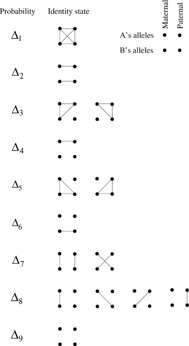
Fifteen possible identity states for individuals A and B, grouped according to their nine condensed states. Lines indicate alleles that are IBD (from Abney et al. 2000).

TABLE 3.

Expressions for the covariances among the genotype indicatorsY_i,g

Genotypes		cov(Yi,g1, Yi,g2)
Covariances between indicators of genotypes g1 and g2 in individual i
g1, g2 = g1		μ0i,g11 − μ0i,g1a
g1, g2 ≠ g1		−μ0i,g1μ0i,g2
g1	g2	covYi,g1, Yj,g2
Covariances between indicators of genotype g1 in individual i and genotype g2 in individual j
k/k	k/k	pkΔij1 + p2kΔij2 + Δij3 + Δij5 + Δij7 + p3kΔij4 + Δij6 + Δij8 + p4kΔij9 − μ0i,k/kμ0j,k/k
k/k	l/l	pkplΔij2 + pkp2lΔij4 + p2kplΔij6 + p2kp2lΔij9 − μ0i,k/kμ0j,l/l
k/k	k/l	Δij3pkpl + 2Δij4p2kpl + Δij8p2kpl + 2Δij9p3kpl − μ0i,k/kμ0j,k/l
k/k	l/m	2Δij4pkplpm + 2Δij9p2kplpm − μ0i,k/kμ0j,l/m
k/l	l/l	Δij5pkpl + 2Δij6pkp2l + Δij8pkp2l + 2Δij9pkp3l − μ0i,k/lμ0j,l/l
k/m	l/l	2Δij6pkpmpl + 2Δij9pkpmp2l − μ0i,k/mμ0j,l/l
k/m	k/m	2Δij7pkpm + Δij8p2kpm + pkp2m + 4Δij9p2kp2m − μ0i,k/mμ0j,k/m
k/m	k/l	Δij8pkpmpl + 4Δij9p2kpmpl − μ0i,k/mμ0j,k/l
k/m	b/l	4Δij9pkpmpbpl − μ0i,k/mμ0j,b/l

^aThe expressions for μ⁰_i,g, expectation of Y_i,g under the null, are given in Table 2 setting r = 0.

Quasi-score test for Hardy-Weinberg equilibrium (QL-HW test):

We propose basing inference on the quasi-score function U (see, e.g., McCullagh and Nelder 1989, Chap. 9):

Here D_r is a [N(M − 1)] vector and D_p is a [(N(M − 1)) × (a − 1)] matrix with the kth column equal to (∂μ/∂p_k). Table 4 gives the expressions for ∂μ_ig/∂r and (∂μ_ig/∂p_k). To construct our Hardy-Weinberg test statistic, we use a similar idea to that used in Bourgain et al. (2003) for the problem of case-control association testing. In analogy with the classical likelihood score statistic when there is a nuisance parameter (see, e.g., Cox and Hinkley 1974, Chap. 9), we use U to build a quasi-score statistic W_QL–HW:

TABLE 4.

Expressions for (∂μ/∂p_k) and (∂μ/∂r) in the case of a locus witha different alleles

Genotype	∂μig/∂pk	∂μig/∂r
k/k	hi + r + 2(1 − hi − r)pk	pk(1 − pk)
l/l	0	pl(1 − pl)
a/a
k/l	2(1 − hi − r)pl	−2pkpl
m/l	0	−2pmpl
a/l	−2(1 − hi − r)pl
a/k

Here I^rr is the (r, r) component of [E(UU^T)]⁻¹, where E(UU^T) is analogous to the information matrix. In our case, the value of r under the null hypothesis is r₀ = 0. p̂₀ is the quasi-likelihood estimate of the nuisance parameter p when r = r₀. In other words, p = p̂₀ is the solution of

3

subject to constraints (1), assuming that there is exactly one such solution. Because we cannot derive a closed-form solution for Equation 3, we obtain p̂₀ by use of the Newton-Raphson method with Fisher scoring as presented by McCullagh and Nelder (1989) for the quasi-likelihood framework. p̂₀ is obtained by iterating

4

until convergence occurs. Here, p̂ⁱ₀ is the approximation to p̂₀ at step i, ∑̂, D̂_p, and μ̂₀ are computed at r = 0 and . To reduce the number of iterations before convergence, we start the iteration procedure with p̂¹₀ equal to the best linear unbiased estimator (BLUE) of p proposed by McPeek et al. (2004). This estimator is based on allele information and does not make use of the additional information of genotypes, i.e., which alleles are paired within the individuals. Finally,

5

where ∑̂, D̂_p, D̂_r, and μ̂₀ are evaluated at r = 0 and p = p̂₀. As demonstrated in Heyde (1997), under the null hypothesis, the quasi-score statistic should follow a χ² distribution with 1 d.f. provided that Var₀(U)^−1/2U ∼ ℳ𝒱𝒩(0, I) under the null hypothesis. We tested the accuracy of the χ² approximation to the null distribution of W_QL–HW (see Null distribution and power study of the W_QL–HW and W_GCC–HW statistics).

To efficiently perform the calculations required in Equation 4, at each step, we take the Cholesky decomposition of ∑̂, i.e., we find an upper triangular matrix B such that B^TB = ∑̂, using an algorithm that simultaneously computes b₀ = B^−TD̂_p and b₁ = B^−T(Y − μ̂₀) at little extra cost (Graybill 1976). Then Equation 4 becomes , where b^T₀b₀ is an [(a − 1) × (a − 1)] matrix, also inverted using its Cholesky decomposition. W_QL–HW is computed with a similar technique in Equation 5.

We conclude this section by describing the form of the QL-HW test statistic in the case of N individuals belonging to F independent families. For each f, 1 ≤ f ≤ F, let N_f be the number of sampled individuals in family f, and let Y_f, μ_f, D_pf, D_rf, and ∑_f be the vectors or matrices previously described but restricted to the N_f members of family f. Allele frequencies are then computed using Equation 4, where and . Similarly W_QL–HW is computed using Equation 5, where all terms of the form X^T∑̂⁻¹B (where X and B are either vectors or matrices) in the formula are computed as .

GCC-HW test:

As the number of alleles per locus and the number of individuals in a family increase, the calculations of the Cholesky decompositions required in (4) and (5) become much more computationally intensive. In practice, with this method, we were not able to analyze Hutterite samples of 400 individuals for loci with more than five alleles. To overcome this limitation, we developed an alternative test, the GCC-HW test, which is computationally simpler than the QL-HW test and therefore suitable for an even wider set of situations (larger samples, larger number of alleles per locus). For outbred samples in the biallelic case, the GCC-HW test is Pearson's Gof-HW corrected using the variance that appropriately accounts for inter-individual correlations. In inbred samples or when considering multiallelic loci, the GCC-HW test is a generalization of this approach. We start by presenting this alternative test in the case of a biallelic locus in an outbred sample with related individuals and present its general expression in a second step. We then clarify how it differs from the QL-HW test.

Special case—corrected χ² test for HW for biallelic loci in outbred samples with related individuals:

Let us first consider a biallelic locus genotyped in an outbred sample with independent individuals. In this case, the QL-HW test is the same as the Gof-HW test, which can be written as , where N_ij is the observed count for genotype ij and p̂_n is the allele frequency estimate of allele 1 obtained by naive counting [p̂_n = (2N₁₁ + N₁₂)/2N].

We next give an equivalent form for Gof-HW in terms of a vector-valued function

which can be left unspecified except that is has the property that

where r₀ = 0. Here D_r, D_p, Y, and μ₀ are the vectors and matrix described in Quasi-score test for Hardy-Weinberg equilibrium (QL-HW test). K is the [(M − 1)N × (M − 1)N] covariance matrix of Y. Because all the individuals are outbred and independent, K is a block-diagonal matrix with K = I_N ⊗ K_ind, where K_ind is a 2 × 2 matrix whose entries depend only on p and are given in the first part of Table 3. It turns out that the Gof-HW test is equal to W_χ²HW, where

6

Here, Ŝ_r is computed at (r, p) = (r₀, p̂₀). p = p̂₀ is the solution of S_p(r₀, p) = 0 and is actually equal to p̂_n. var̂₀S⁻¹_rr denotes the (r, r) entry of var(S)⁻¹ computed at (r, p) = (r₀, p̂₀). It is actually equal to 1/N.

One way to extend (6) so that it is valid when the individuals are related is to consider the same S(r, p) function (with K = I_N ⊗ K_ind, thus neglecting the inter-individual correlations) and to recompute var̂₀S⁻¹_rr to take the inter-individual correlations into account. We have var₀(Y) = ∑, with elements given in Table 3, where all h_i = 0 in this case. Using and noting that for outbred individuals, we get , where ∑̂, K̂, and D̂_r are computed at (r, p) = (r₀, p̂₀) (here again, p̂₀ = p̂_n). We assess the accuracy of the χ² approximation to the null distribution of this corrected χ² (W_CC–HW) statistic in Null distribution and power study of the W_QL–HW and W_GCC–HW statistics.

General form of GCC-HW test:

There does not appear to be a Pearson χ² test corresponding to the HED model for multiallelic loci. Furthermore, in the case of inbreeding, while one can extend the Gof-HW test to allow for a mean level of inbreeding, it does not take into account the different inbreeding coefficients for different individuals. To generalize the W_CC–HW statistic, we consider the following framework. Let

and define

r̂

p̂

to be the solution of C(r, p) = 0 subject to constraints (1) and (2), assuming that there is exactly one such solution. Although the framework is more general, we consider here C to be the form

7

for some invertible matrix L that may depend on r and p, with D_i, L, and μ not depending on Y. Assume that

r̂

p̂

is consistent for the parameters

r

p

of the HED model and is asymptotically normal. Following the arguments used by Cox and Hinkley (1974)(Chap. 9) to derive the score test, under certain regularity conditions, we consider the expansion of C(r, p) in a Taylor series about

r̂

p̂

where

Then,

8

and

9

Under the assumptions made on

r̂

p̂

,

10

should have an asymptotic χ² distribution with dim(r) d.f. Here

is the (r, r) entry of var

r̂−r

p̂−p

. To test the null hypothesis r = r₀, we plug in r = r₀ in (10). p is a nuisance parameter and we use its restricted estimator p̂₀, where p = p̂₀ is the solution of C_p(r₀, p) = 0, subject to constraints (1), assuming that there is exactly one such solution. Under certain regularity conditions, this is asymptotically equivalent to the case when the true p is used.

The W_GCC–HW statistic has the general form defined in (10), where C(r, p) is given by (7) with L set to K, the matrix defined in the subsection Special case—corrected χ² test for HW for biallelic loci in outbred samples with related individuals.

are approximated with Equations 8 and 9, respectively. Doing so, we can consider the same HED model as the one used in the QL-HW test, which allows a distinct h_i for each individual, by simply using for μ the model described in Table 2. To test for HW, we use r₀ = 0. The K matrix used in C(r, p) is the covariance matrix of Y where the intra-individual correlations are taken into account but where the inter-individuals correlations are neglected. Thus, K is still a block diagonal matrix but with distinct matrix elements K_i of size (M − 1) × (M − 1), whose entries depend on p and h_i, and K⁻¹ is a block-diagonal matrix with matrix element K⁻¹_i. We show in the appendix that W_GCC–HW reduces to , where Ĉ_r = C_r(r₀, p̂₀) and

11

computed at (r, p) = (r₀, p̂₀). In outbred samples, p̂₀ corresponds to the naive counting estimator in which allele frequencies are estimated by their observed proportions. In inbred samples, C_p(r₀, p) = 0 may not have a closed-form solution, in which case we use the Newton-Raphson method, as we did for the QL-HW test: p̂₀ is obtained by iteration using Equation 4, where ∑ is replaced by K. We start the iteration procedure with p̂¹₀ equal to the BLUE (McPeek et al. 2004) computed under the pretense that all the individuals have their correct inbreeding coefficients but are independent. Note that, because D_r^TK⁻¹D_p = 0 when considering a biallelic locus in an outbred sample, W_CC–HW is a special case of W_GCC–HW. Whereas the computation of W_QL–HW requires the Cholesky decomposition of ∑, a covariance matrix of size [(M − 1)N × (M − 1)N], the computation of W_GCC–HW requires only the Cholesky decompositions of the N K_i matrices of size [(M − 1) × (M − 1)]. It is thus much less computationally intensive. Similarly to the W_QL–HW quasi-score statistic, we assess the accuracy of the χ² approximation to the null distribution of W_GCC–HW in results.

When the N individuals belong to F independent families, W_GCC–HW and p̂₀ are computed using the same formulas as in the one-family case presented above but with all the terms of the form X^TK̂⁻¹∑̂K̂⁻¹B computed as .

Explanation of the difference between QL-HW and GCC-HW:

Because both have an appropriate variance correction, both QL-HW and GCC-HW are valid tests that are approximately χ² distributed in sufficiently large samples under regularity conditions. The difference is that, in the definition of GCC-HW, the matrix K is plugged in for L in Equation 7, while in the definition of QL-HW, the matrix ∑ is plugged in for L. This difference potentially affects the power of the statistics. For instance, by an argument similar to that given in Bourgain et al. (2003), the QL-HW should be asymptotically more powerful than GCC-HW for local alternatives (i.e., alternatives close to the null hypothesis) under certain regularity conditions, assuming that the HED model holds, and, in fact, should be asymptotically locally most powerful of all statistics of the type defined by Equation 7. We compare actual power of GCC-HW and QL-HW under simulated scenarios in results.

Null distribution and power study of the W_QL–HW and W_GCC–HW statistics:

To test the accuracy of the χ² approximation to the null distributions of the W_QL–HW and W_GCC–HW statistics, we assessed their distributions under the null hypothesis using (i) a sample of 30 outbred independent nuclear families with two parents and two sibs typed (sample nuc), (ii) a sample of 456 individuals from 10 extended outbred genealogies (sample gaw), and (iii) two samples of 611 (sample H1) and 306 (sample H2) Hutterites. The 10 extended genealogies were simulated for the Genetic Analysis Workshop 12 (Almasy et al. 2001). The different genealogies are independent but the mean within-genealogy kinship coefficient is 0.0415 ([0.030–0.054]). The Hutterites are a North American religious isolate originating from Tyrol whose entire population can be traced back to 90 ancestors in the 1700s/1800s. The complete genealogy of the sample could be constructed from a ≥12,000-person Hutterite pedigree. This yielded a 1623-person pedigree that included all known ancestors of the individuals in samples H1 and H2. The nine identity coefficients for all pairs of individuals, from which the inbreeding coefficients can also be obtained, were computed using the efficient algorithm implemented by Abney et al. (2000). Genotype information for a marker was simulated by randomly drawing alleles independently from the same allele frequency distribution for (i) the parents of the nuclear families or (ii) the founders of the 10 genealogies or (iii) the founders of the 1623-person pedigree. Mendelian transmission of these alleles was then simulated (i) in the nuclear families, (ii) in the 10 genealogies, or (iii) throughout the 1623-person pedigree. The validity of the χ² null distribution for W_QL–HW and W_GCC–HW was assessed by comparing the proportion of simulations showing a statistic whose value is greater than the χ² threshold for a nominal type I error and the value of this nominal type I error. For the outbred nuc and gaw samples, the empirical type I error of the classical Gof-HW test was also assessed, using either the χ² distribution or a permutation procedure (where alleles are randomly reassigned to genotypes 5000 times) to obtain significance.

For the Hutterite samples, in addition to the χ² approximation, we also had to develop a parametric bootstrap procedure to assess significance, as follows: for a given data set, we estimated the allele frequencies (p̂_data) using Equation 4 (with ∑̂ for W_QL–HW and K̂ for W_GCC–HW) and computed the value of the statistic W_data (either W_QL–HW or W_GCC–HW). p̂_data was then used to simulate 5000 replicates of the original data set under the null hypothesis (following the procedure described in the previous paragraph). The statistic was computed in each replicate. The empirical significance was assessed as the proportion of simulated statistic values greater than W_data. In principle, one could double-check the type I error of this parametric bootstrap procedure by performing a nested set of simulations, but we did not attempt this for computational reasons.

Simulations were also used to assess power. Even though HW testing is used mostly to identify potential genotyping errors in SNP studies, generating a genotyping error model would also have created Mendelian incompatibilities. As Mendelian incompatibilities are routinely checked before any other test, considering such a genotyping error model would have implied evaluation of a combined Mendelian checking/HW testing approach, whereas we wanted to focus solely on HW testing. Thus, we chose to consider a model without Mendelian incompatibilities. Further, we required this model to be suitable for samples with fixed genealogy. We simulated a selection pattern where the allele transmission from parent to offspring is not equally likely for the two parental alleles (we retain independence of children's genotypes conditional on parents' genotypes). For a biallelic marker, a single parameter 0 < s < 1 is required to describe our model. Table 5 gives the corresponding transmission probabilities from parents to offspring as a function of s. Here, we considered the situation where, for parental couples who are compatible with both homozygous and heterozygous children, the probability that any given child is heterozygous is greater than would be expected under Mendelian inheritance: s > ¹/₂. Power was assessed in the samples nuc, H1 and H2 using 5000 replicates. For the Hutterite samples, founders' alleles were simulated assuming HWE in the founding population, with founding allele frequency taken to be 0.5, 0.7, or 0.85. In the case of nuc, we assume that the families are sampled from a population that is in a steady state for our selection model. We give in Table 6 the population genotype frequencies corresponding to this steady state in an infinite-size population under random mating. When s > ¹/₂, the genotype frequency distribution depends only on s and not on p (whatever the initial allele frequency, p = 0.5 in the steady state). The parental genotypes of the nuc families were sampled independently from the steady-state genotype distribution for various choices of s > 0.5. In such a nuclear family sampling scheme, the classical Gof-HW test would consider only the 60 independent parents. To measure the gain in power obtained while using QL-HW on the global sample instead of the Gof-HW test on the parent sample, we derived analytically the power of the Gof-HW test using a noncentral χ² distribution.

TABLE 5.

Parent/offspring transmission model used to mimic selection in the power computations

Parental genotypes (Gp)	Offspring genotype (Go)	Pr(Go|Gp)*
ii × ii	ii	1
ii × jj	ij	1
ii × ij	ii	1 − s
	ij	s
ij × ij	ii	(1 − s)/2
	jj	(1 − s)/2
	ij	s

^*Probability of offspring genotype conditional on parental genotypes.

TABLE 6.

Steady-state genotype frequencies for the selection model presented in Table 5 under random mating, for a biallelic locus, as a function ofs and of the initial allele frequencyp

Genotypes	11	12	22
s = 1/2	p2	2p(1 − p)	(1 − p)2
s > 1/2	(−1/2 + 1/2a)/(1 − 2s)	(2(1 − s) − a)/(1 − 2s)	(−1/2 + 1/2a)/(1 − 2s)
s < 1/2
p = 1/2	(−1/2 + 1/2a)/(1 − 2s)	(2(1 − s) − a)/(1 − 2s)	(−1/2 + 1/2a)/(1 − 2s)
p < 1/2	0	0	1
p > 1/2	1	0	0

With .

Analysis of biallelic markers:

We used the W_QL–HW statistic to test for HW in a set of 143 biallelic markers in 82 genes that were genotyped in samples of Hutterites. A variety of genotyping methods were used: multiplex PCR and immobilized probe linear array system (LAS) (Mirel et al. 2002) for 48 markers (34%), single base extension with fluorescent polarization (SBE-FP; Chen et al. 1999) for 44 markers (31%), dot blot with allele-specific oligos (Ober et al. 2000) for 26 markers (18%), restriction fragment length polymorphism analysis (RFLP) for 13 markers (9%), size separation on acrylamide gel for 9 insertion/deletion (in/del) polymorphisms (6%), allele-specific (AS) PCR for 1 marker (0.7%), SSCP (Gonen et al. 1999) for 1 marker (0.7%), and denaturing high-performance liquid chromatography (DHPLC; Oefner and Underhill 1995) for 1 marker (0.7%). All markers were checked for Mendelian incompatibilities in the general pedigree using PEDCHECK (O'Connell and Weeks 1998).

RESULTS

Null Distribution of the W_QL–HW and W_GCC–HW statistics:

Table 7 presents the empirical type I error of the classical Gof-HW, W_QL–HW, and W_GCC–HW statistics in the outbred samples of nuclear families and in the extended outbred genealogies. The classical Gof-HW test, whatever the significance procedure used, either the χ² distribution or the permutation test, is anti-conservative. While the inflation in the type I error is moderate in the nuclear families (type I error of 7% instead of 5%), it becomes substantial in the extended GAW12 genealogies (type I error of 10%). In contrast, when the χ² distribution is used to assess significance of the W_QL–HW or W_GCC–HW statistics, the empirical type I error lies within the 95% confidence interval of the nominal type I error (5%) for all three allelic distributions considered in the founders. In the two Hutterite samples (results shown in Table 8), the empirical type I error for both W_QL–HW and W_GCC–HW is smaller than the nominal one. Use of the χ² approximations to the null distributions of the statistics would thus lead to conservative tests in the Hutterite sample. We note, however, that when simulating a sample consisting of 10 independent copies of the 1623-person Hutterite pedigree and running the two statistics on a sample of 6110 Hutterites (10 times sample H1), the empirical type I error for a biallelic locus with frequency 0.5 in the founders is not statistically different from the nominal one when assuming a χ² distribution. Similarly, when considering only 2 outbred genealogies out of the 10 from the gaw sample (corresponding to 106 individuals deriving from 41 founders), the χ² distribution provides valid type I errors for both the W_QL–HW and the W_GCC–HW tests. The asymptotic conditions required for the W_QL–HW and W_GCC–HW to have a χ² distribution under the null hypothesis should thus be met in most samples, except in the extreme case where all the individuals belong to a single inbred pedigree. In this case, the central limit theorem either may not apply or may require a larger sample size to be a good approximation, and the test may be conservative. We give in Table 8 the thresholds corresponding to a 5% nominal type I error, for three different allelic distributions, in the two Hutterite samples. These thresholds vary with sample sizes and allele frequencies. We would thus recommend use of empirical P-values obtained by the parametric bootstrap (as described in methods), for samples in which all the individuals come from a single inbred pedigree.

TABLE 7.

Empirical type I error of the classical χ² goodness-of-fit test for HWE with significance assessed using either the χ² distribution or a permutation procedure and of theW_QL–HW andW_GCC–HW statistics with significance assessed using the χ² distribution, for a 5% nominal type I error

	Statistic:	Gof-HW		WQL–HW:	WGCC–HW:
Allele frequency	Significance with:	χ2 distribution	Permutation	χ2 distribution	χ2 distribution
Nuclear families
0.50		0.073	0.075	0.051	0.052
0.70		0.072	0.074	0.053	0.053
0.85		0.070	0.073	0.046	0.044
GAW12 genealogies
0.50		0.103	0.102	0.050	0.049
0.70		0.099	0.102	0.052	0.049
0.85		0.086	0.094	0.047	0.042

Estimates are based on 5000 simulations in a sample of 30 outbred nuclear families (nuc) and in a sample of 456 individuals from 10 extended genealogies of the GAW12.

TABLE 8.

Empirical type I error of theW_QL–HW andW_GCC–HW statistics for a 5% nominal type I error and 5% corrected threshold, in two different Hutterite samples: H1 (611 individuals) and H2 (306 individuals)

		Empirical type I error				5% corrected thresholdb
Statistic:	WQL–HW		WGCC–HW		WQL–HW		WGCC–HW
Allele frequencya	Sample:	H1	H2	H1	H2	H1	H2	H1	H2
0.50		0.017	0.029	0.020	0.026	2.61	3.00	2.83	3.00
0.70		0.017	0.015	0.014	0.024	2.55	2.71	2.58	2.85
0.85		0.008	0.018	0.003	0.009	2.21	2.59	1.88	2.18

Estimates are based on 5000 simulations.

^aAllele frequency distribution from which the alleles of the pedigree founders are drawn.

^bUncorrected threshold is 3.84.

Power of the W_QL–HW and W_GCC–HW statistics:

Figure 2 displays the power of W_QL–HW in the nuc sample (30 nuclear families) for values of s varying between 0.5 and 0.75, where power was computed using the χ² approximation. Figure 2 also displays the power of the Gof-HW test in the sample of 60 independent parents that can be extracted from the nuclear families. The gain in power obtained while using W_QL–HW instead of Gof-HW can be substantial: when s = 0.65, the power of W_QL–HW is 79% instead of 55% for the Gof-HW test. There is still a notable increase in power at more realistic values of s close to 0.5. The power of W_GCC–HW was also computed for the nuc sample, but it is not shown in the plot as the results were almost indistinguishable from those for W_QL–HW. Thus, the simpler W_GCC–HW appears to be approximately as powerful as the W_QL–HW in this sampling scheme. Because they allow one to use all the information available in the families and thus to increase the sample size, the QL-HW and GCC-HW tests may significantly enhance the power to detect HWD when familial data are available.

Figure 2.—

Power of the QL-HW test in 30 nuclear families (solid line) and power of the Gof-HW test in the corresponding parent sample (dashed line), as a function of s, for a 5% type I error.

In the Hutterite sample, founder genotypes are not available, so the Gof-HW test in founders cannot be performed. Thus, we compare power only for the W_QL–HW and W_GCC–HW tests. To see a power difference between the two tests, we set s = 0.6, even though this value is probably unrealistically high for selection in a human population. Table 9 displays the results, where significance is assessed using a correct 5% nominal threshold obtained by simulation under the true model (the thresholds are shown in Table 8). For the purpose of simulation studies, this method of assessing significance was used because it is much faster than the parametric bootstrap that we use in the real data examples. Because the same method is used with both statistics, we expect this to have a negligible impact on the power comparison. The W_QL–HW performs slightly better than the W_GCC–HW in the Hutterite samples; however, the power difference between the two tests is quite small. Thus, use of W_GCC–HW instead of W_QL–HW in situations in which W_QL–HW cannot be computed (e.g., a highly polymorphic marker in a pedigree with many individuals typed) should not have too strong an impact on power. Conversely, W_QL–HW should be preferred when computable. Note that the power of both methods in the Hutterite samples is expected to increase when the allele frequency becomes closer to 0.5. Indeed, as can be seen from Table 5, our model is such that selection acts only when there is at least one heterozygous parent. When the allele frequency becomes closer to 0.5, the proportion of heterozygous parents increases and the impact of selection increases as a result.

TABLE 9.

Power of theW_QL–HW andW_GCC–HW statistics for different allele frequency distributions in two Hutterite samples (H1 and H2) withs = 0.60

Sample	H1			H2
Allele frequencya	0.5	0.7	0.85	0.5	0.7	0.85
WQL–HW	0.92	0.88	0.76	0.78	0.76	0.63
WGCC–HW	0.90	0.88	0.76	0.78	0.73	0.62

Nominal type I error is 5%; estimates are based on 5000 simulations.

^aAllele frequency distribution from which the alleles of the pedigree founders are drawn.

Marker testing for HWE in the Hutterites:

The results for the 14 markers, of the 143 biallelic markers tested, that showed an associated P-value <5% by the W_QL–HW are shown in Table 10. Four of these markers (HLA-G_689, LTA_26, OR12D2_2, OR2H3_587) are located within the HLA region, which has been associated with homozygous deficiencies in this population (Robertson et al. 1999). The genotyping methods used to type the 14 markers in Table 10 were not very different from those used to type the 143 markers except that the only marker typed with allele-specific PCR was among the 14 markers with a P-value ≤0.05, markers typed by LAS were underrepresented (34% of all markers but only 14% of the markers with a P-value ≤0.05), and markers typed by dot blot were overrepresented (18% of all markers but 28% of the markers with a P-value ≤0.05) (see Figure 3). Thus, it is unlikely that any particular genotyping method was more error prone or contributing disproportionately. We further investigated the genotyping history of these 14 markers. Two markers, HLA-G_689 and OR12D2_2, produced an excess of Mendelian errors and had already been either discarded (for OR12D2_2) or retyped using another method (for HLA-G_689). Two additional markers, PSG4_1 and PLAUR_210, had a high rate of ambiguous genotypes. Overall, it is likely that the deviations from HWE for these 4 markers were due to genotyping errors, although only 2 were previously identified as problematic by Mendelian error checking.

TABLE 10.

Results of theW_QL–HW test in the Hutterites for the 14 biallelic markers with an associated empiricalP-value ≤0.05

Marker name	Genotyping method	rs no.	Sample size	Allele frequency	WQL–HW P-value
PLAUR_210a	Dot blotc	RS2302524	604	0.85	0.0002
PON1_55	LASd	RS85460	646	0.74	0.003
PSG4_1a	Dot blotc	RS4028448	306	0.52	0.015
C5_802	SBE-FPe	RS17611	394	0.51	0.015
ZFR_1	SBE-FPe	RS714932	758	0.67	0.023
IL4R_-3223	AS PCRf	RS2057768	413	0.68	0.027
LTA_26b	LASd	RS1041981	671	0.83	0.028
NIDDM1_43	Dot blotc	RS3792267	675	0.68	0.034
ESE-3_50834	in/delg	RS4987414	504	0.51	0.036
IL4R_1597	Dot blotc	RS15987825	410	0.56	0.036
OR12D2_2a,b	SBE-FPe	—	632	0.52	0.039
HLA-G_689a,b	SBE-FPe	RS2735022	679	0.56	0.041
ZFR_3	RFLPh	RS889318	681	0.66	0.042
OR2H3_587b	SBE-FPe	RS3129034	672	0.71	0.043

Genotyping methods and dbSNP rs numbers are shown. Exact P-values are computed with 5000 simulations.

^aMarkers for which genotyping errors are suspected.

^bMarkers in the HLA region.

^cDot blot with allele-specific oligos.

^dMultiplex PCR and immobilized probe linear array system.

^eSingle-base extension with fluorescent polarization.

^fAllele-specific PCR.

^gSize separation on acrylamide gel.

^hRestriction fragment length polymorphism analysis.

Figure 3.—

Proportion of markers typed with the eight different genotyping methods for the set of 143 SNPs tested (solid bars) and for the 14 SNPs with an associated P-value ≤0.05 (open bars).

Finally, the remaining 10 markers with a P-value ≤0.05 of 143 (6.9%) represent slightly more than what is expected just by chance (but the observed proportion is not significantly different from 5% at the 5% level). Given that the P-values associated with each of these 10 markers are not dramatically small and that we had at least 1 other marker typed in 9 of these genes that was not significant, we believe that the small deviations from expectation in these 9 genes might be due to chance. We cannot rule out, however, that these departures reflect the real action of evolutionary forces.

DISCUSSION

We demonstrated in this article that the classical Gof-HW test has inflated type I error in samples with related individuals when significance is assessed either with a χ² approximation or with a permutation test. Sing and Rothman (1975) previously discussed the problem of testing for HWE in small human populations with nonnegligible correlations among the individuals. Whereas they corrected the expectation of the χ² in a very particular case of correlation among the observations, we propose in this article a general approach suitable for any sample with related individuals provided that their genealogy is known. Our QL-HW test models the correlation between the two alleles of each individual due to the pedigree structure and, by making use of the quasi-likelihood framework, takes into account the correlations among the individuals in the construction of the test.

We chose to base our test on the model of heterozygote excess or deficiency studied by Rousset and Raymond (1995), and we extended it to allow a different inbreeding coefficient for each individual in the sample. In the context of SNP studies, where deviations from HWE are likely to result from genotyping errors, our model is very general in allowing for deviations from HWE. For multiallelic markers, our model specifically tests for an excess or a deficiency of homozygosity. A primary reason for choosing such a model is parsimony. Furthermore, it is motivated by previous findings using microsatellites in which excess of all kinds of heterozygotes has been observed, in particular in the HLA region (Ober et al. 1997; Robertson et al. 1999). This model is also relevant for detection of genotyping errors. Indeed, as noted by Sobel et al. (2002), when automated software or trained technicians genotype by scoring bands on a gel, the most common error is false homozygosity. An error occurs in this case when an allele amplifies insufficiently or a band falls outside a prescribed range. In addition, these authors also discuss the possibility of false heterozygosity when a stutter band is misinterpreted as a second allele. Thus, we expect our model to be useful for detecting genotype errors in the cases of both SNPs and multiallelic markers. Alternatively, a model involving more parameters could be incorporated into our quasi-likelihood score test framework, if the available evidence favored such a model.

We also propose a simpler alternative test, the GCC-HW test, to be used when the QL-HW test might not be computationally feasible, for instance, in the case of highly polymorphic loci in large inbred pedigrees. We found that for a variety of study designs, ranging from many nuclear families to two or more extended genealogies, the χ² approximation to the null distributions of both the QL-HW and the GCC-HW was very accurate. It was only in the extreme case of a single large inbred pedigree that the tests were rather conservative. In that case, we recommend using the parametric bootstrap to assess significance. Further, we showed that the use of the GCC-HW test in place of the QL-HW test has only a very minor effect on the power to detect deviation from HWE. Finally, we illustrated on nuclear family data how the QL-HW test can improve the power to detect departure from HWE over the classical Gof-HW test.

We believe that, by making the HWE test available for a larger variety of samples and by increasing sample sizes through the inclusion of related individuals that are typically discarded, both the QL-HW and GCC-HW tests are of crucial interest in several relevant situations for geneticists. In particular, as illustrated by the data analysis presented here, HWE testing is an additional tool for genotyping error detection. Indeed, of the four markers with HWD and strong suspicion of typing errors after scrupulous checking, only two had been previously detected by regular Mendelian error checking. We thus strongly recommend that HW tests be routinely performed to detect genotyping errors, particularly while working with SNPs. Finally, used very cautiously, the QL-HW and GCC-HW tests could also be considered as possible tools to detect association in samples with related individuals. The program to run the QL-HW and GCC-HW tests is available on request from C.B. (dbSNP home page, http://www.ncbi.nlm.nih.gov/SNP/index.html).

APPENDIX:

EXPRESSION OF W_GCC–HW

To derive W_GCC–HW, we need to evaluate (r̂ − r) and

at (r, p) = (r₀, p̂₀) using approximations (8) and (9), respectively, which require the computation of A ≡ ÊC′ r, p⁻¹_r0,p̂0 and B ≡ var̂Cr, pr₀, p̂₀. We use the notation

It follows from (7) with L = K that , , and . Because C_p(r₀, p̂₀) = 0 and letting Ĉ_r = C_r(r₀, p̂₀), (8) implies that r̂ − r|_r0,p̂0 ≈ α^rrĈ_r. Similarly, (9) implies

Note that and , where . Plugging these expressions in (10) gives, after some algebra, the final expression of den_GCC given in (11).

References

- Abney, M., M. S. McPeek and C. Ober, 2000. Estimation of variance components of quantitative traits in inbred populations. Am. J. Hum. Genet. 66 629–650. [DOI] [PMC free article] [PubMed] [Google Scholar]
- Almasy, L., J. D. Terwilliger, D. Nielsen, T. D. Dyer, D. Zaykin et al., 2001. GAW12: simulated genome scan, sequence, and family data for a common disease. Genet. Epidemiol. 21 S332–S338. [DOI] [PubMed] [Google Scholar]
- Bourgain, C., S. Hoffjan, R. Nicolae, D. Newman, L. Steiner et al., 2003. Novel case-control test in a founder population identifies P-selectin as an atopy susceptibility locus. Am. J. Hum. Genet. 73 612–626. [DOI] [PMC free article] [PubMed] [Google Scholar]
- Chen, X., L. Levine and P. Y. Kwok, 1999. Fluorescence polarization in homogeneous nucleic acid analysis. Genome Res. 9 492–498. [PMC free article] [PubMed] [Google Scholar]
- Cox, D. R., and D. V. Hinkley, 1974 Theoretical Statistics. Chapman & Hall, London.
- Douglas, J. A., A. D. Skol and M. Boehnke, 2002. Probability of detection of genotyping errors and mutations as inheritance inconsistencies in nuclear-family data. Am. J. Hum. Genet. 70 487–495. [DOI] [PMC free article] [PubMed] [Google Scholar]
- Gonen, D., J. Veenstra-VanderWeele, Z. Yang, B. L. Leventhal and E. H. J. Cook, 1999. High throughput fluorescent CE-SSCP SNP genotyping. Mol. Psychiatry 4 339–343. [DOI] [PubMed] [Google Scholar]
- Graybill, F. A., 1976 Theory and Application of the Linear Model. Duxbury Press, North Scituate, MA.
- Heyde, C., 1997 Quasi-Likelihood and Its Application: A General Approach to Optimal Parameter Estimation. Springer-Verlag, New York.
- Jacquard, A., 1974 The Genetic Structure of Populations. Springer-Verlag, New York.
- Lange, K., 1997 Mathematical and Statistical Methods for Genetic Analysis. Springer-Verlag, New York.
- Lee, W. C., 2003. Searching for disease-susceptibility loci by testing for Hardy-Weinberg disequilibrium in a gene bank of affected individuals. Am. J. Epidemiol. 158 379–400. [DOI] [PubMed] [Google Scholar]
- McCullagh, P., and J. A. Nelder, 1989 Generalized Linear Models, Ed. 2. Chapman & Hall, London.
- McPeek, M. S., X. Wu and C. Ober, 2004. Best linear unbiased allele-frequency estimation in complex pedigrees. Biometrics 60 359–367. [DOI] [PubMed] [Google Scholar]
- Mirel, D. B., A. M. Valdes, L. C. Lazzeroni, R. L. Reynolds, H. A. Erlich et al., 2002. Association of IL4R haplotypes with type 1 diabetes. Diabetes 51 3336–3341. [DOI] [PubMed] [Google Scholar]
- Nielsen, D., M. G. Ehm and B. Weir, 1999. Detecting marker-disease association by testing for Hardy-Weinberg disequilibrium at a marker locus. Am. J. Hum. Genet. 63 1531–1540. [DOI] [PMC free article] [PubMed] [Google Scholar]
- Ober, C., L. R. Weitkamp, N. Cox, H. Dytch, D. Kostyu et al., 1997. HLA and mate choice in humans. Am. J. Hum. Genet. 61 497–504. [DOI] [PMC free article] [PubMed] [Google Scholar]
- Ober, C., S. A. Leavitt, A. Tsalenko, T. D. Howard, D. M. Hoki et al., 2000. Variation in the interleukin 4 receptor a gene confers susceptibility to asthma and atopy in ethnically diverse populations. Am. J. Hum. Genet. 66 517–526. [DOI] [PMC free article] [PubMed] [Google Scholar]
- O'Connell, J. R., and D. E. Weeks, 1998. PedCheck: a program for identification of genotype incompatibilities in linkage analysis. Am. J. Hum. Genet. 63 259–266. [DOI] [PMC free article] [PubMed] [Google Scholar]
- Oefner, P. J., and P. A. Underhill, 1995. Comparative DNA sequencing by denaturing high-performance liquid chromatography (DHPLC). Am. J. Hum. Genet. 57 A266. [DOI] [PubMed] [Google Scholar]
- Robertson, A., D. Charlesworth and C. Ober, 1999. Effect of inbreeding avoidance on Hardy-Weinberg expectations: examples of neutral and selected loci. Genet. Epidemiol. 17 165–173. [DOI] [PubMed] [Google Scholar]
- Rousset, F., and M. Raymond, 1995. Testing heterozygous excess and deficiency. Genetics 140 1413–1419. [DOI] [PMC free article] [PubMed] [Google Scholar]
- Sing, C. F., and E. D. Rothman, 1975. A consideration of the chi-square test of Hardy–Weinberg equilibrium in a non-multinomial situation. Ann. Hum. Genet. 39 141–145. [DOI] [PubMed] [Google Scholar]
- Sobel, E., J. C. Papp and K. Lange, 2002. Detection and integration of genotyping errors in statistical genetics. Am. J. Hum. Genet. 70 496–508. [DOI] [PMC free article] [PubMed] [Google Scholar]
- Weinberg, C., and R. W. Morris, 2003. Invited commentary: testing for Hardy-Weinberg disequilibrium using a genome single-nucleotide polymorphism scan based on cases only. Am. J. Epidemiol. 158 401–403. [DOI] [PubMed] [Google Scholar]
- Weir, B. S., 1996 Genetic Data Analysis 2: Methods for Discrete Population Genetic Data, Ed. 2. Sinauer Associates, Sunderland, MA.
- Xu, J., A. Turner, J. Little, E. R. Bleecker and D. A. Meyers, 2002. Positive results in association studies are associated with departure from Hardy-Weinberg equilibrium: Hint for genotyping error? Hum. Genet. 111 573–574. [DOI] [PubMed] [Google Scholar]