Using Temporally Spaced Sequences to Simultaneously Estimate Migration Rates, Mutation Rate and Population Sizes in Measurably Evolving Populations

Abstract

We present a Bayesian statistical inference approach for simultaneously estimating mutation rate, population sizes, and migration rates in an island-structured population, using temporal and spatial sequence data. Markov chain Monte Carlo is used to collect samples from the posterior probability distribution. We demonstrate that this chain implementation successfully reaches equilibrium and recovers truth for simulated data. A real HIV DNA sequence data set with two demes, semen and blood, is used as an example to demonstrate the method by fitting asymmetric migration rates and different population sizes. This data set exhibits a bimodal joint posterior distribution, with modes favoring different preferred migration directions. This full data set was subsequently split temporally for further analysis. Qualitative behavior of one subset was similar to the bimodal distribution observed with the full data set. The temporally split data showed significant differences in the posterior distributions and estimates of parameter values over time.

DRUMMOND et al. (2002, 2003a) treat joint estimation of mutation rate, population size, and sample genealogies from time-stamped serially sampled sequence data, using a Bayesian approach and Markov chain Monte Carlo (MCMC). In this article we extend this method to fit an island migration model (Notohara 1990). We focus on the case of two populations. We model asymmetric migration rates and unequal population sizes using serial samples of sequences.

Software tools for estimating migration parameters from DNA sequence data exist. These include Migrate (Beerli and Felsenstein 1999, 2001), GenTree (Bahlo and Griffiths 2000), and MDIV (Nielsen and Wakeley 2001). These methods use MCMC to obtain maximum-likelihood estimates of migration rates and population sizes, but apply only to sequences obtained at a single time. As a consequence these methods estimate the composite parameter Θ = 2Nμ (here N is the effective population size and μ the mutation rate).

We focus on measurably evolving populations (MEPs; Drummond et al. 2003b). Sequences of a given locus are sampled from individuals in a population on several sampling occasions. By definition, MEPs show a statistically significant increase in the number of substitutions over the sampling interval (Drummond et al. 2003b). The human immunodeficiency virus (HIV) type I is a MEP. Serial samples taken from a single patient over a period of years show rapid accumulation of mutations in the viral genome and the generation of a large number of genetic variants. HIV forms distinct subpopulations in different body tissues, for example, in the brain and in the blood (Wong et al. 1997; Poss et al. 1998; Wang et al. 2001; Zhang et al. 2002). Serially sampled sequence data, labeled by subpopulation, are therefore available. With HIV, the presence of different tissue compartments may signal the availability of reservoirs of virus that can hamper the effectiveness of antiviral therapy (Nickle et al. 2003). It is therefore important to understand the pattern of HIV compartmentalization in the body and the timing of these “colonization” events.

Our method differs from the methods employed by Bahlo and Griffiths (2000) and Beerli and Felsenstein (2001). Because we work with time-stamped sequence data, and MEPs, we can estimate population, migration, and mutation parameters simultaneously and separately (Rodrigo and Felsenstein 1999; Drummond and Rodrigo 2000). We use a Bayesian framework rather than a maximum-likelihood approach. This allows scientists using this approach to incorporate prior information as they deem appropriate. Such prior information may include knowledge about the means and variance of mutation rates or the most plausible direction of migration. Physically irrelevant parameter ranges, such as populations of size very much smaller than one, must be ruled out explicitly. This imposes an additional discipline on the inference.

Our work may be thought of as a methodologically straightforward but technically demanding extension of Drummond et al. (2002)(2003a) to handle the island migration model. We apply our algorithms to a set of simulation studies. This tests software and identifies quantities poorly resolved by the data. We compare our results with results obtained by other authors. We then treat a real HIV data set, drawn from blood and semen samples, from a single patient taken at four time points over the period of 3 years. The data are rich in features of interest. We use them to illustrate the way the tools we have provided may be used to explore such data sets. We are unwilling, however, to make too many strong inferences about HIV biology on the basis of our analyses, because the complexities of HIV evolution present constant challenges to such analyses. In particular, our analyses ignore selection, recombination, and changes in population size, all of which will have significant impact on the results.

The outline is as follows: in island-model genealogies and mutation we describe the island model of migration and its likelihood for serially sampled sequences. In bayesian inference, we determine a posterior distribution for the parameters of interest. The MCMC integration tools we used to sample and summarize that distribution are described in markov chain monte carlo for migration genealogies and code implementation and verification. In selected results from simulated data, we present the results of the simulation studies and finally hiv patient data is devoted to real HIV sequences obtained from two tissue compartments in a single patient over a number of time points. MCMC details are given in the appendix.

ISLAND-MODEL GENEALOGIES

We now describe the probability density for a Fisher-Wright population model (Fisher 1930; Wright 1931) using the Kingman coalescent (Kingman 1982a,b) extended to include migration (Hudson 1990; Notohara 1990) and nonisochronous (i.e., serial or time stamped) leaf tips. For an analysis of the properties of the isochrone model, see Hudson (1990) and Notohara (1990) and references therein.

The island model of migration is a model of p populations, or demes. For j ∈ 𝒟, 𝒟 = {1, 2 … , p}, deme j is a panmictic population of N_j haploid individuals. Time increases into the past and is measured in calendar units. Let λ_ij denote the per capita migration rate from deme i to j (time increases into the past, so in forward time the individual is moving from j to i).

The migration process we describe below is a process that realizes migration-coalescent genealogies under the island model of migration. A migration-coalescent genealogy g is a rooted and directed binary tree graph with four node types: n leaf nodes (with label set ℒ) of in-degree one and out-degree zero, n − 1 coalescent nodes (label set 𝒞) of which n − 2 have in-degree one and out-degree two and one (the root, label R say) has in-degree zero and out-degree two, plus an indeterminate number, m say, of migration nodes (label set ℳ) of in-degree one and out-degree one. Let 𝒜 = 𝒞∪ℳ denote the set of all ancestral (i.e., nonleaf) node labels and V = ℒ∪𝒜 denote the set of all node labels. Tree edges 〈r, s〉 are directed toward the present. Let E denote the set of all edges in the tree graph and V_−R = V \{R} the set of all node labels excluding the root.

Individuals corresponding to leaf nodes are sampled from the demes. Deme labels are recorded. Because the observation process is conditioned on the scientist's sampling of individuals over demes, the number of individuals sampled from a deme need not reflect the deme size. For r ∈ ℒ, suppose individual r was sampled from deme i_r ∈ 𝒟 at calendar time t_r. The event represented by node r ∈ 𝒜 occurred at calendar time t_r. Nodes are labeled from r = 1 to r = m + 2n − 1 in order of increasing age and by least child label in case of ties, so that r > s ⇒ t_r ≥ t_s and 〈r, s〉 implies t_r ≥ t_s. For any set X ⊂ V let t_X = (t_X, r ∈ X), with entries ordered by increasing r. Let t = t_V. Let |X| denote the number of elements in set X.

Let ρ equal the mean number of units of calendar time per generation. We do not estimate ρ; instead we present results for a nominal ρ. For example, for the HIV data set in hiv patient data, t_r is measured in days before an arbitrary zero and we set ρ = 1 day.

The demographic process realizing migration-coalescent tree graphs is defined as follows. An ancestral lineage is associated with each sampled individual and carries a label indicating deme membership. As time increases into the past, each lineage in deme i migrates independently of all other lineages at rate λ_ij to deme j. Each pair of lineages in deme i coalesces at instantaneous rate 1/θ_i, where θ_i = N_iρ. The process terminates when the number of lineages equals one. With each event we associate a node, r ∈ 𝒜, and with each lineage between events an edge 〈r, s〉 ∈ E. For each s ∈ V_−R, let i_s give the deme on edge 〈r, s〉. Let 𝒥 = (i₁ … i_m+2n−2) be the set of all deme edge labels and 𝒥ℒ and 𝒥𝒜, respectively, the sets of deme labels for edges {〈r, s〉 ∈ E, s ∈ ℒ} and {〈r, s〉 ∈ E, s ∈ 𝒜} attached to leaf and ancestral nodes. Let λ = (λ_1,2 … λ_p−1,p) and θ = (θ₁ … θ_p). A visual representation can be seen by skipping ahead to Figure 4, where the leaf deme membership is shown with either a dashed line for one deme or a solid line for the other deme. Migration nodes (events) are where the line changes deme (line type); otherwise it is a traditional coalescent genealogy.

Figure 4.—

Typical trees realized by MCMC simulation of the full data set. (—) Blood deme; (---) semen. (Top) Trees from the s → b mode; (bottom) b → s mode.

The free and conditioned parameters of a migration genealogy g are (E, 𝒥𝒜, t_𝒜) given (𝒥ℒ, t_ℒ). Because the data 𝒥ℒ and t_ℒ are known and fixed throughout the analysis, and leaf labels are determined from the label-time ordering, we write g = (E, 𝒥, t) and keep in mind that some of the parameters in g are fixed. The parameter set 𝒥 is subject to constraints determined from the leaf demes. When there are just two demes, the deme labels 𝒥𝒜 are uniquely determined from the event topology E by propagating the demes from the leaves to the root (switch deme at each migration event). Let Γ denote the set of all admissible migration genealogies g, which can be realized by the migration-coalescent process above, for given 𝒥ℒ and t_ℒ. Γ is the union over m of sets Γ_m containing all migration genealogies with m migration events. Note that the Euclidean dimension of the space Γ_m is m + n − 1 (one dimension for each time variable t_r, r ∈ 𝒜) and as a consequence, Γ is a union of spaces of unequal dimension.

We now write the joint density f(g|θ, λ) for a migration tree (the corresponding distribution is given in appendix A). Consider the interval of time δ_r = t_r+1 − t_r between consecutive nodes on the tree. There are m + 2n − 2 such intervals on a tree g ∈ Γ_m, one interval above each node r ∈ V_−R (for isochronous leaves, δ_r = 0 for r = 1, 2 … n − 1). For i ∈ 𝒟 and r ∈ V_−R, let k_ir denote the number of lineages in deme i in interval r. For i ∈ 𝒟, let 𝒟_−i = 𝒟\{i} denote the set of demes omitting deme i. For each r ∈ V_−R, the interval (t_r, t_r+1] contributes a factor

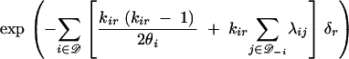to the density, along with a second factor equal to 1/θ_i or λ_ij as the event type at time t_r+1 is coalescent in deme i or (i → j) migration. An interval terminated by a leaf (when r + 1 ∈ ℒ) ends in a nonevent, and the second factor is one. Let m_ij denote the total number of (i → j) migrations, i.e., m_ij = |{r ∈ ℳ; i_r = j, i_ř = i}| with ř the child node of migration node r in g. Let c_i denote the total number of coalescent events in deme i, with ř₁ and ř₂ the child nodes of coalescent node r in g. The overall density is

We note a few distributional details relevant to the MCMC over migration genealogies. Technically, f(g|θ, λ) is the density of a distribution f(g|θ, λ)dg. If g has m migration events then 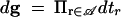is the element of volume in Γ_m. Migration and coalescent events are distinguished by their position on the tree and we take counting measure over topologies and 𝒥-labels conditioned on leaf properties. The density given above is normalized, ∫_Γf(g|θ, λ)dg = 1.

The migration coalescent generalizes the Kingman coalescent. Free movement or strong migration (Nagylaki 1980; Notohara 1993) is signaled by λ_ij ≫ 1/θ_j. Model populations with high migration rates can still be structured, as migration imbalance determines a source and sink population structure. If in addition, for each deme j ∈ 𝒟, the local immigrant and emigrant population fluxes balance,

the aggregate population evolves as one panmictic population of size ∑_j∈𝒟N_j.

MUTATION

Mutation rate, μ, is inferred with our method by incorporating the traditional mutation model. We use the finite sites mutation model, with neutral selection and general time reversible (GTR) substitution process of Felsenstein (1981) and Rodriguez et al. (1990). The substitution process is a continuous-time Markov process with states {A, C, G, T}, a 4 × 1 vector of equilibrium probabilities π, and a 4 × 4 rate matrix Q normalized to generate one substitution per unit calender time (−∑_dπ_dQ_dd = 1). The substitution and migration processes are independent.

Each leaf node r ∈ ℒ has associated with it nucleotide sequence data D_r = (D_r,1, D_r,2, D_r,3, … , D_r,L) of length L with D_r,a ∈ {A, C, G, T, φ} for a = 1, 2, … , L. Gaps, indicated by φ, are treated as unobserved sites. Let D_ℒ be the n × L matrix of sequences on the leaves.

The likelihood PD_ℒ|g, μ is defined and computed in the usual way, using node-to-node transition probabilities (Felsenstein 1981). For these purposes migration nodes may be ignored and we consider the topology in the traditional sense. We calculate the likelihood PD_ℒ|g, μ in the usual manner using pruning (Felsenstein 1981).

BAYESIAN INFERENCE

In this section we set out Bayesian inference for μ the mutation rate, the vector θ of N_iρ-values, and the vector λ of migration rates. The migration genealogy g may be of direct interest also. The joint posterior density of these variables

1

is given in terms of the likelihood function P, the migration genealogy prior f, a prior p on μ, θ and λ, and z, an unknown and intractable normalization constant. Here h is the density of a distribution h(λ, θ, μ, g) dλdθdμdg with dλ = dλ_1,2dλ_1,3 … dλ_p−1,p and dθ = dθ₁dθ₂ …dθ_p.

Subjective, informative priors are a fundamental part of Bayesian inference. However, we want to set out a new parameter estimation scheme for a new data-model pair (namely serial sequence data in an island migration model). Informative priors can hide certain difficulties users will face when they apply Monte Carlo Bayesian inference. First, MCMC convergence is more easily achieved as the sampled probability density is more concentrated in its space of states. For example, the bimodality that makes the HIV data of hiv patient data such a challenge to MCMC, and such a good pedogogical example, can be removed by adding prior information. Second, diffuse priors that are actually improper can lead to improper posteriors and meaningless results. In the last paragraphs of this section and in hiv patient data we explain how an improper posterior could but does not arise in our case. Improper priors put mass on physically irrelevant parameter values. Should not a prior worth the name rule out such states? Certainly. However, suppose that is achieved via a simple cutoff in parameter space. We want to know whether results are sensitive to the choice of cutoff. If the posterior is improper without the cutoff then parameter estimates will be strongly influenced by the choice of cutoff. We should take particular care in choosing the cutoff and make a sensitivity analysis. Just this scenario arises in hiv patient data. Third, when we form parameter estimates using Bayesian inference we should test each data set with several priors and make many entire MCMC analyses of each data set, not just one. What is the range of inferential outcomes that result from approaching these data with different subjective prejudices? How do conclusions change as we move from an informative to a more diffuse prior? Fourth, priors that seem to be noninformative can turn out to be strongly informative for some hypotheses. For example, an improper prior on genealogies assigns equal probability density to all rooted trees with n leaves. This prior is noninformative for comparison of unique tree topologies. However, the marginal prior density of the root time t_R in this prior is tⁿ⁻²_R. This prior is very strongly informative for root time. Diffuse priors bring special problems. We choose examples in which those problems are present so that we can show how to deal with them. We regard our explanations of how to deal with these problems as an integral part of our exposition of the methodology itself.

Note that we are estimating rates for mutation, migration, and coalescence simultaneously from a single data set. Drummond et al. (2002) have shown that mutation rate μ and population size θ_i = N_iρ parameters may be separated when sequenced individuals are sampled serially over a timescale long enough to see mutational change. This is feasible for populations, such as HIV, that are measurably evolving. Drummond et al. (2003a) give conditions for the estimation problem to be well defined in the absence of migration. This issue needs to be considered when priors are improper. We bound θ_iμ, i ∈ 𝒟, μ, and λ_ij above and below. (Note that we bound the traditional parameter Nρμ, but this implies a bound on θ.) In this setting any density of bounded range determines a proper posterior. Note that panmictic populations lead to migration rates λ_ij large compared to 1/θ_j. Bounds must allow such parameter values or the panmictic condition will be eliminated by the prior. We bound λ_ij above so that the number of migrations per generation does not exceed one, λ_ijρ ≤ 1, relying on a fixed estimate for ρ. This allows λ_ij as large as about N_j/θ_j (depending on the accuracy of the estimated generation time), while still providing the upper bound on migration rate needed for posterior normalization.

The upper bound (or upper tail) imposed on θ_i, i ∈ 𝒟, by the prior plays an important role in the inference. Migration genealogies containing no coalescent events in deme i ∈ 𝒟 [so c_i = 0 in f(g|θ, λ)] make up a set S_i ⊂ Γ of nonzero posterior probability p_i, say. Now, for each g ∈ S_i there is ε(g, i) so that f(g|θ, λ) > ε(g, i) for all θ_i ≥ 0. In other words, for each demographic parameter θ_i there is a component of the posterior in which the distribution of θ_i at large values is controlled only through the prior p(μ, θ, λ). These physically irrelevant parameter values, corresponding to populations of negligible size, must be ruled out explicitly. It follows that if, for example, the θ_i priors are untruncated uniform (or otherwise nonintegrable) priors on θ_i ≥ 0, the posterior cannot be proper. An example of this posterior sensitivity to prior bounds is discussed in detail at the end of hiv patient data. A lower bound on λ_ij plays a similar role for Jefferys priors (of the form 1/X for parameter X). In that case the problem arises where tree states with no migration events in one direction m_ij = 0 have nonzero probability, the likelihood is bounded away from zero as λ_ij → 0, and the posterior has the form 1/λ_ij at small λ_ij. Again, unphysical parameter values must be ruled out explicitly.

MARKOV CHAIN MONTE CARLO FOR MIGRATION GENEALOGIES

The posterior density h is summarized using samples drawn from h via Metropolis Hastings Markov chain Monte Carlo (MCMC; Metropolis et al. 1953; Hastings 1970). The constant z does not need to be evaluated. The main challenges we encountered are the classic obstacles of MCMC-Bayesian inference, the bimodality apparent in some parameters, and a posterior distribution that is very close to being improper. We discuss these issues below. In appendix A we describe a Metropolis-Hastings algorithm that determines a Markov chain X_n, n = 0, 1, 2, … , with unique equilibrium distribution coinciding with the posterior distribution. The arguments ψ = (λ, θ, μ, g) of the posterior density function h make up the state vector. The MCMC acceptance probability we write in Equation A1 is a slightly simplified form of the Metropolis-Hastings-Green acceptance probability of Green (1995). The number of migration events in the state ψ is randomly variable, and as a consequence the tree-component g of the MCMC state must jump between subspaces g ∈ Γ_m, which are, as we note above, of unequal dimension. The Metropolis-Hastings-Green generalization of the usual Metropolis-Hastings algorithm treats this feature.

The MCMC operators used to transform the state are called “moves.” We implemented ∼10 distinct move types. At each MCMC step we choose one of these moves according to some random schedule and apply it to the state. See appendix A for details. We omit detailed descriptions of moves specified in Drummond et al. (2002). Where a tree-topology change is proposed, it is necessary to check that the candidate state is legal (identical deme label for all edges in E attached to every coalescent node). Our candidate generation ignores deme labels. Any candidate state that was not a legal migration-coalescent genealogy was rejected and the MCMC was counterincremented. Such rejections are computed rapidly and appear to give good mixing per CPU cycle, even in the case of many demes (four). Addition and deletion of migration nodes were implemented using a pair-birth/death operation (A4) and a pair-split/merge operation (A5). These moves are illustrated in Figure 1. These operators give irreducibility over migration node number and position for two demes. With the migration birth/death operation (A3) these moves allow the MCMC to visit any migration history of a given coalescent tree with three or more demes. A set of now standard coalescent tree operators (Drummond et al. 2002) gives irreducibility over Γ. Mixing over the parameters μ, θ, and λ of the mutation and demography models is achieved via scaling moves, that is, by taking random multiples. This is just random-walk MCMC carried out on a log scale. The two advantages of scaling MCMC are, first, that the size of the change is automatically at the scale of the parameter and, second, that the posterior distribution is insensitive to certain scaling transformations (so t/θ is invariant under t → δt, θ → δθ). Tricks of this kind are discussed in detail in Drummond et al. (2002).

Figure 1.—

Two basic migration moves used in our MCMC implementation. (A) Two migration nodes or events are either deleted or added to a single edge. (B) The migration event is “moved” through a coalescent node.

Moves that are simple may give adequate mixing per CPU second if they can be evaluated quickly. Such moves may be relatively easy to implement accurately. We found that we were able to treat at least some problems of practical interest with the simple moves listed in appendix A. Operations on migration nodes are fast, as no likelihood change is involved.

In the experiments reported in selected results from simulated data and hiv patient data, we restrict attention to populations spread over just two demes, so that p = 2 and 𝒟 = {1, 2}. The first real two-deme data set we looked at was rich in features of potential methodological and biological interest, so we have chosen to display our work in this setting. In the two-deme problem, the deme type i_s ∈ 𝒟 of each edge 〈r, s〉 is determined uniquely from 𝒥ℒ, the leaf deme values. The MCMC moves in appendix A treat p ≥ 2. There are two simplifications to the MCMC moves for p = 2. First, the migration birth/death operation (A3) is not required (the MCMC parameters are fixed so that it is selected with probability zero at the proposal step). Second, there is a deme-selection step in the pair-birth move that is uniform at random from the set of demes that might admissibly occupy the new position. It will be seen that this set has just one member in the binary case, so the admissible deme is selected with probability one.

Suppose we iterate the MCMC J steps, collecting samples ψ_s every S steps for a total N = J/S samples. A MCMC realization of this kind is called a “run.” We estimate f̂ = N⁻¹∑_sf(ψ_s). It is important to have reliable estimates of var{f̂} to debug MCMC, that is, to determine whether the difference between f̂ and E_h{f(ψ)} is significant. We follow Geyer (1992). The uncertainty in our estimate f̂ depends on the integrated autocorrelation time τ_f. Since var{(f̂)} = τ_fvar{(f)}/N, τ_f can be interpreted as the number of correlated MCMC samples f(ψ_s) with the same variance-reducing effect as one independent sample. We estimate τ_f from the lag a autocorrelation function γ_a = cov(f(ψ_s), f(ψ_s+a))/var(ψ_s) using the monotone sequence estimator described in Geyer (1992). We report the effective sample size (ESS) N/τ_f for a few statistics computed from our MCMC runs to give a quality check on the MCMC. Efficiency comparisons can be decided from estimated integrated autocorrelation times. Let c denote the mean number of CPU seconds per update. The program with the smallest cτ_f-value is generating iid-equivalent samples f(ψ_s) most rapidly.

It is necessary to check that the MCMC has reached equilibrium and that the variance estimates discussed in the preceding paragraph are reliable. We make multiple independent MCMC runs r = 1, 2, … , R, from starting conditions drawn independently from the ψ-prior. We evaluate a f̂_r for each run and check that the between-run variance of f̂ is predicted by its in-run variance. When we report results in selected results from simulated data and hiv patient data, we superimpose histograms of f(ψ) computed from the R independent runs. We inspect traces, f(ψ_s) as a function of s, for any visual evidence of a trend. We perform a number of further checks as described in Geyer (1992).

CODE IMPLEMENTATION AND VERIFICATION

The program was written in the JAVA programming language. JAVA was chosen primarily because of its portability and object-oriented features. MCMC is computationally very intensive, so some effort went into tuning performance. However, correctness and ease of debugging were prioritized ahead of performance.

A number of tests were used to verify and debug the code. Naturally we checked that we could recover parameter values from synthetic data, for a wide range of parameter values. Our set of MCMC moves includes moves that are not needed for irreducibility. We check that the simulated posterior density does not change as we vary the proportions in which moves are used. We used the MCMC to simulate the prior density f(g|θ, λ) for migration-coalescent trees. Independent samples from this density can be obtained by backward simulation of the migration-coalescent process. A number of statistics [for example, t_R = max(t) and m = |ℳ|] were checked in this way and were found to have excellent agreement.

SELECTED RESULTS FROM SIMULATED DATA

The results of 150 simulated data sets are summarized in Table 1. The first set of simulation studies (top of the table) is for symmetric migration rates and population sizes, where this restriction was relaxed for the second set of simulation studies. The details of each are now discussed.

TABLE 1.

Means of the modes, standard deviation of the modes, and coverage estimators for relevant parameters of 25 simulated data sets each

s/ca	True θ, λ	θ	σθ	% coverage	λ	σλ	% coverage	μ	σμ	% coverage
c	0.05, 2	0.05124	0.008339	92	2.278	1.579	100	—	—	—
c	0.05, 200	0.04976	0.007293	100	248.7	135.44	100	—	—	—
s	0.05, 2	0.04937	0.008226	92	1.832	1.270	100	0.9723	0.06115	100
s	0.05, 200	0.04832	0.006364	92	194.7	98.9	96	0.972	0.05112	96
N1, λ1 → 2, s	0.1, 1	0.1006	0.02805	90	1.078	1.039	100	1.013	0.4470	100
N2, λ2 → 1, s	0.2, 10	0.2054	0.04405	90	11.04	3.343	100
N1, λ1 → 2, s	0.2, 1	0.2111	0.05082	92	1.509	1.939	96	0.9935	0.05762	92
N2, λ2 → 1, s	0.1, 10	0.1001	0.02510	100	12.13	4.559	100

Where serial sequences are used, μ is included. All run lengths were three million states while some runs were longer; see the text for details. The last four rows show the asymmetric simulations.

^aSerial samples (s); contemporary samples (c).

Symmetric migration and population sizes:

For simplicity of exposition and to connect with earlier work, we take two identical demes. We suppose that the migration rates either way and population sizes are known a priori to be equal. In the next section we treat a more general estimation problem. We set λ_1,2 = λ_2,1 = λ and θ₁ = θ₂ = θ. We make two pairs of studies, corresponding to parameter estimation in the weak (λ = 2, θ = 0.05, λ < 1/θ) and strong (λ = 200, θ = 0.05, λ > 1/θ) migration regimens. The MCMC sampling problem becomes harder as the posterior mean λ increases, as the mean and variance of the number of migration events (about 300 in our strong migration example) increases. In each migration regime we consider serial and isochronous leaf data. We consider isochronous leaf data to allow readers to compare our results with previous studies, in particular, Beerli and Felsenstein (1999). For serial data we estimate λ, θ, μ, and g. For isochronous data, θ and μ are confounded. In that setting we condition on knowledge of μ and estimate λ, θ, and g. We tried Jeffreys priors and uniform priors for λ, θ, and μ with conservative upper bounds. Results presented are for Jeffreys priors, but were in any case very similar.

In each of the four studies we generate 25 migration-coalescent trees. Each tree has 50 leaves, with 25 individuals in each deme. On each tree we simulate synthetic sequence data using a GTR model with fixed relative rate matrix (Shankarappa et al. 1999; normalized to unit mean total substitution rate). This rate matrix is appropriate for HIV and is used in the study of real HIV data presented in the next section. All sequences were 1000 bp long and the mutation rate μ was set equal to one. For the serial data the 50 leaves were split into two groups of 25, offset in time by 0.1 time units (since data are synthesized with μ = 1, these time units happen to be substitutions per site). The earlier sample set was made up of 12 sequences from subpopulation 1 and 13 from subpopulation 2. The MCMC runs were 3 million states long. The worst mixing (by far) was observed for serial data with λ = 200, where there are a large number of migration events on the tree, and μ and θ are estimated separately. For this group of 25 synthetic data sets, each MCMC run was monitored for convergence, and terminated when appropriate, rather than run as a batch for a predetermined number of updates. Run times varied between 2 and 10 hr with run lengths up to 8 million updates. ESS values depend on the particular realization of synthetic data, varying between 25 and 200 for μ and 10 and 100 for λ.

Results are summarized in Table 1, top. For each study we report the proportion of the 25 trials in which the true parameter values were inside the 95% highest posterior density (HPD) confidence set. We uncover the truth as we had hoped. Figure 2 shows the marginal posterior density for migration of a typical MCMC run. It is a skewed unimodal distribution. For this reason we used a mode estimator on the marginal posterior density. There is a slight bias, of the same kind observed by Beerli and Felsenstein (1999) in studies of the likelihood for isochronous data. Mode estimation was accomplished by noting that the local density is inversely proportional to the spread of a fixed number of adjacent point samples. We note that the mode is generally a much better point estimator of the true value than mean estimators used in other articles. Contour plots of 95% migration parameters of representative samples from isochronous and serial leaf data are shown in Figure 3. The isochronous data give migration rate estimates that are both less precise and more strongly skewed than migration rate estimates derived from serial data.

Figure 2.—

A typical marginal density plot for simulated data for λ. In this example θ = 0.05 and λ = 2.

Figure 3.—

Approximate 95% HPD confidence contour plots for representative synthetic data runs. True values are θ = 0.05 and λ = 2 indicated by crosshairs. (A) For serial samples; (B) for isochronous samples. Note reduced variance at B.

Asymmetric migration rates and population sizes:

Two simulated studies relaxed the original constraint of symmetric population size and migration rates. A total of 60 taxa were used, and the true values tested are λ₁ = 1, λ₂ = 10 and θ₁ = 0.1, θ₂ = 0.2 while for the second set the population size parameters were reversed to θ₁ = 0.2, θ₂ = 0.1. In all other aspects the simulation setup was the same as that for the symmetric case above except as noted below.

The reason for the increase in taxa was to obtain informative confidence interval estimates; otherwise they would often be very like the prior. Table 1, bottom, gives the results for the two-parameter sets and shows good recovery of the truth. Generally the convergence and variance are less favorable for this case and longer runs were required (∼5 million); otherwise the qualitative behavior is similar to that described above.

HIV PATIENT DATA

In this section we present an analysis of a real data set. We have chosen HIV sequence data from a single patient. Four sets of samples were collected from two viral demes (blood and semen) over a period of 3 years yielding 31 blood (b-deme) and 25 semen (s-deme) sequences of length 638. The distribution of leaf demes across time can be seen from the line type at the leaf tips in Figure 4.

In the following analysis we use a GTR substitution model with the same fixed rate matrix used for the synthetic data. We do not assume, as we did above, that the two populations are behaving in the same way. The migration rates and population sizes are all distinct. We have 𝒟 = {blood, semen}, p = 2, and parameters λ = (λ_s,b, λ_b,s), θ = (θ_s, θ_b), μ, and g.

We began by making some exploratory runs on the complete data set, varying priors and start-state and pseudo-random number initialization between runs. The key feature is bimodality in migration rate parameters. The Markov chain state ψ = (λ, θ, μ, g) flips between two different interpretations of the data. Figure 5A shows the behavior of the parameter λ_s,b along a 200 million update segment of a 540 million update run. In this run the λ, θ and μ priors were flat and bounded at conservative values. The λ_s,b-parameter is jumping between two quite different values. All parameters jump in concert with λ_s,b. This posterior distribution has two well-defined peaks. This is visible in a contour plot of the joint posterior λ_s,b, λ_b,s|D distribution, Figure 5B.

Figure 5.—

Some plots for the full HIV data set. (A) Plot of λ_s→b for the full HIV data set showing 400 million of the total 540 million updates. Flat bounded priors were used. (B) The migration contour plot from the same data clearly showing the bimodality.

What is the origin of the bimodality? The simplest possibility is that the data tell us that the migration is asymmetric, but leave the favored direction in doubt. Uncertainty of this kind can be removed, if further prior knowledge is available; as noted in the Introduction, with appropriate information, we may weight the asymmetry of rates in favor of one or the other direction of migration. On the other hand, the MCMC might be failing us. Perhaps there is no real bimodality and the MCMC is not in equilibrium. We consider also the possibility that the model is wrong. In particular the population sizes and per capita migration rates may change with time. Also the blood deme may in fact be multiple unobserved demes, which we discuss below in more detail.

Figure 4 gives typical genealogies for the respective modes. At the top is a tree from the s → b (λ_b,s > λ_s,b) mode. There are in forward time many migration events, most of which are s → b and close to the leaves (so λ_b,s is large). At the bottom is a tree from the b → s mode (λ_s,b > λ_b,s). There are fewer migration events, most of which are b → s. There are no important changes in the topology of coalescent events between modes.

Trees in the b → s mode have fewer migration events than those in the s → b mode. In the s → b mode, the proximity of many s-deme leaves to the root supports an s-deme for the root. Coalescent branches terminating in b-deme leaves are typically much longer than those terminating in s-deme leaves. This feature is particularly marked in the topmost b-clade associated with the last two time stages in the data set (compare it with the s-clade for those two stages). Because so much of the total branch length is close to b-deme leaves, the s → b events needed to convert the s-deme at the root are most probably located close to the leaves. This statement has been checked by analyzing the simple but related problem of estimating the relative rates of a two-state mutation process on a fixed tree. Extending the leaf branches raises the likelihood of asymmetric rate estimates. This kind of reconstruction (many migration events close to leaves) was never seen in synthetic data on simulated trees. It is seen in synthetic data generated on trees, like those in Figure 4, simulated from the posterior of this HIV data set. It seems likely that the bimodality is related to the long branches attached to the blood-deme leaves.

Why are the branches attached to the blood deme stretched in this way? We may be seeing a model violation. The blood deme may be a composite of several unobserved demes. The likely consequence of multiple, hidden demes is to lengthen the time to coalescence of any two lineages, i.e., to lengthen the branch lengths. As we note above, the apparent relationship between bimodality and long branches may therefore be a reflection of the fact that we have not sampled from these hidden demes. Other aspects of HIV evolution can also account for long branches; for instance, both population growth and recombination have the characteristic effect of producing long terminal lineages, consistent with the patterns we observe here.

In the remainder of this section we rule out the possibility that the bimodality is a consequence of software artifacts and insufficient mixing of the Monte Carlo chain. In these bimodal runs, the MCMC state is moving between two classes of migration genealogies that differ by the number and position of a large number of nodes (∼60). The intermediate states have low probability. It is the bimodality of this data set rather than its size that puts it at the limit of what we can study with this software on current hardware. The states make sense as alternative explanations of the given leaf deme types. This basic consistency, with positive results for the MCMC convergence checks described in markov chain monte carlo for migration genealogies, convinces us that the bimodality is real and that the MCMC is delivering states representative of the posterior.

We search now for evidence of time dependence in λ and θ. We separate the data into two sets. The “new” (“old”) data set contains sequences from all individuals sampled at the two “last” (“first”) time stages. The MCMC mixes far more rapidly on these data sets. Effective sample sizes in the hundreds are obtained from overnight runs and we were able to make a more thorough study. For each of these data sets we made 20 runs with random starting states and 500 million updates per run, sampling every 10,000 states. Of the 20 runs, 10 used flat priors and 10 used scale invariant Jeffreys priors. Conservative hard upper bounds were imposed in all cases. Figure 6 shows the estimated autocorrelation function computed from the MCMC output for μ in the new data set with flat priors and was typical. These statistics yielded a worst-case parameter ESS of 1300, the smallest effective sample size over all runs.

Figure 6.—

Autocorrelation function γ_s (defined in markov chain monte carlo for migration genealogies) for μ for the new data set. The x-axis is sample number (multiply by 10,000 to get updates). This plot indicates (i.e., good) typical mixing.

Selected marginal posterior plots are shown in Figures 7 and 8. Marginal posterior densities are consistent between runs, which supports other evidence that the MCMC runs have equilibrated. The time to equilibrium was a tiny fraction of the run length. The bimodality present in the full data set is visible in Figure 10, the new data set, which tends to support the view that it represents a real ambiguity in the data, rather than an artifact of time-varying demography. When the migration genealogies associated with the two modal classes of the new data set are examined, we see the same qualitative behavior as for the full data set, which is shown in Figure 9.

Figure 7.—

Marginal posterior density for μ in old (right-hand peak) and new (left-hand peak) data sets. Note the decrease in mutation rate with time.

Figure 8.—

Marginal λ_s→b in the old data set. The higher peak was obtained using Jeffreys priors and the lower one using flat priors.

Figure 10.—

Contour plots of migration rates for temporally split data sets. (A) The new data set (note the bimodality). (B) The old data set.

Figure 9.—

Instances of trees from the new data set MCMC chain showing bimodality similar in character to the full data set. Analysis of the old data set does not show bimodality.

Comparison of the two data sets does reveal significant differences in parameter values. Referring to Figure 7, the mutation rate is higher in the old data set. We have used a constant nominal generation time ρ equal to 1 day. The mutation rate depends on generation time, which in turn is dependent on the type of cell infected: broadly, HIV-infected cells can be classified into three categories—productively infected cells, long-lived cells, or latently infected cells (Perelson et al. 1996). Each of these categories has different generation times, the shortest being productively infected cells (on the order of 2 days) and the longest being latently infected cells (on the order of several years). It is conceivable that as infection progresses, the relative proportions of these infected cells change in the tissues sampled, thus leading to a change in observed mutation rates. Migration is strongly s → b in the early part of the infection, but only weakly asymmetric in the later stages, possibly reflecting a higher rate of early colonization events, before the saturation of available target cells in semen (Figure 10).

Figure 11B illustrates the general point that the switch from flat to Jeffreys priors has little consequence for marginal posterior densities. In Figure 11B we see that the Jeffreys prior does pull in the upper tail of the θ_s-distribution fairly sharply. This sensitivity of the upper tail of the θ_i-distribution to the choice of prior can be understood as follows. Bounds can be set to conservative values without particular care if the MCMC output is studied carefully. Where MCMC runs actually visit bounds, we have a possible signal that the data are adding little to the information in the prior. The parameter θ_sμ visits its upper bound (at N_sρμ = 0.5); since μ ≈ 0.2 × 10⁻⁵ this bound acts around θ_s ≃ 0.5/0.2 × 10⁻⁵ ≃ 25,000. This is visible in Figure 11A, where θ_s exceeds the plotted range. This is just what we expect from the discussion in bayesian inference concerning migration genealogies with no coalescent events in a given deme [the c_i parameter of f(g|θ, λ) is zero with posterior probability p_i] for the flat prior used for that run. If p_i is very small, the MCMC θ_i-trace will not visit the tail of the posterior density made up of states associated with c_i = 0, even though (for the flat prior) that tail does not die to zero as θ_i → ∞. For the full HIV data set this is the case. The posterior mean θ-values will diverge as the prior upper bound is sent to infinity but the problem is not visible in the MCMC because the corresponding p_i-values are negligible. However, in the new component of the data set, both p_s and p_b are sufficiently large. The long tail in the θ_s-distribution for the flat prior in Figure 11B and the spiky excursions to the upper bound at θ_sρμ = 0.5 are instances of the phenomenon. Care needs to be taken to ensure that the upper tail of the prior θ_i, i ∈ 𝒟, distributions really represent prior knowledge. No Bayesian inference that is completely noninformative of θ_i can be made. Where the MCMC does not reveal the true tail behavior, as in the full data runs, the best we can do is assert that we have enough evidence to know what we would see if we waited long enough.

Figure 11.—

New data set plots for θ_s. (A) One MCMC trace and (B) multiple marginal plots. The higher peak in B was obtained using Jeffreys priors and the other using flat priors. Despite the appearance of bad mixing, we note the excellent agreement between chains in B.

DISCUSSION

We have shown that we can simultaneously recover mutation rate, population sizes, migration rates, and genealogical information from temporal and spatially sampled sequence data within a Bayesian framework using MCMC. This nontrivial problem involving a space of varying dimension has been shown to converge in practical time frames with complex data sets of moderate size.

Simulation results demonstrated that recovery of the true parameters is consistent and repeatable with rapid convergence for low (λ < 1/θ) migration rates. The case of large migration (λ ≥ 1/θ) convergence is slow due to the large number of migration events on the genealogy, frequently exceeding 500.

A real HIV data set was also analyzed to further demonstrate the method. It was found that the joint posterior density was bimodal on exploratory runs. This bimodality could be understood as a consequence of the coalescent tree shape, which the sampled sequences determine. The very long leaf branches attached to blood-deme individuals raise the likelihood for an interpretation that would otherwise have low probability, an interpretation putting many s → b migration events on those long branches. As a consequence, the data do not distinguish the preferred direction of migration. This conclusion was supported by results obtained when the data set was split temporally. The same qualitative behavior was observed in one of the data sets. Joint posterior distributions were successfully recovered from both time “sets” and were shown to be reasonably insensitive to priors.

Parameters, in particular the mutation rate, vary from the earlier to the later data set. This is particularly important, because it demonstrates the need to take account of the fact that the values of some or all evolutionary parameters may change over time. With MEPs it becomes possible to model these changes explicitly (see, for instance, Drummond et al. 2001). In fact, allowing evolutionary parameters to change over time permits us to model some biologically interesting phenomena. For instance, if we allow migration rates to change from zero to nonzero values as one moves backward in time, we can simulate vicariant biogeographic events that may precede speciation. Alternatively, with ancient DNA samples obtained from glacial refugia, one may be able to model both the onset of glaciation and the consequent restriction to gene flow, followed by the period of subsequent recolonization. Modeling these types of changes, while potentially challenging from a MCMC perspective, poses no theoretical obstacle.

However, the fact that we have not incorporated changes into the present model also makes us wary about making too many inferences on the basis of our analysis of the real HIV data set. In particular, it is reasonable to assume that as infection of a new compartment proceeds, population size in that compartment will increase. We have not factored such increases into our analyses. Nor have we taken account of positive selection acting on the HIV genome. The complexity of HIV evolution challenges simple models of inference. For this reason, we view such models as stepping stones to reality.

APPENDIX:

MARKOV CHAIN MONTE CARLO MOVE TYPES

We now present the details of our MHMCMC implementation. We do not cover the moves already presented in Drummond et al. (2002). We note that where such a move results in an illegal state due to migration constraints, the move is rejected, and for a small number of demes (four or less) this gives reasonable acceptance rates (i.e., very similar to the original moves performance). Generally acceptance rates were quite low for some moves, but still gave acceptable ESS per CPU cycle because of the very quick evaluation of the acceptance ratio. All tunable parameters were not difficult to adjust and both the simulated data and HIV data gave similar overall acceptance rates of ∼20%. The MCMC scheme used was reversible jump MCMC; see Green (1995)(2003) for further details.

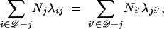
Suppose X_n = ψ. We refer to n as the MCMC update counter. X_n+1 is determined in the following way. Move k is chosen, with probability r(k), from a fixed set of state operators. Let u = (u₁, u₂, …) denote an ordered list of independent uniform variates. Let T_k(ψ, u) = ψ′ denote a move T generating the new state ψ′. We suppose that there is k′ for which r(k′) > 0 and T_k′(ψ′, u′) = ψ for some u′. With some probability α(ψ′, ψ) set X_n+1 = ψ′, and otherwise set X_n+1 = ψ. The acceptance probability α is chosen to ensure that the Markov process is reversible with respect to h. Following Green (1995) set

A1

The requirement that the last term, which is the Jacobian for the change of variables from (ψ, u) to (ψ′, u′), must be nonsingular, is called the dimension-balancing condition. Let

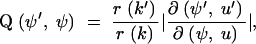A2

so that α(ψ′, ψ) = min{1, Q(ψ′, ψ)h(ψ′)/h(ψ)}. It is convenient, for the variable dimension MCMC, to drop the convention that the nodes labels are time ordered. Nodes carry their labels as they are operated on by MCMC moves. The maximum label need not equal m + n − 1.

Joint scale move:

This move was needed to obtain acceptable μ-mixing. Fix 0 < β < 1 and draw δ uniformly at random from [β, 1/β]. The candidate state ψ′ is

where . The leaf times are not scaled, since they are data. If the move produces an invalid state (child older than parent), the move is rejected. Otherwise the move is its own inverse and Q(ψ′, ψ) = δ^{1+p−p(p−1)/2+m+n−1−2}; that is, Q = δ^|𝒜^|−1 when p = 2 since |𝒜| = m + n − 1. We found that β = 1.1 − 1.2 gave good acceptance ratios (∼20%).

More general scale moves:

We employed a number of variants of the joint scale move described above. Variables were scaled individually and in randomly chosen groups. This amounts to a collection of random-walk operations that act on the log scale. As an example, the μ-variable is updated as follows. Fix 0 < β_μ < 1. If the scale-μ update is chosen, δ is drawn uniformly at random from [β_μ, 1/β_μ]. The candidate state ψ′ is

The Hastings-Green factor is Q(ψ′, ψ) = 1/δ. The real variables λ, μ, and Θ and the t_𝒜 parameters of g were all updated in this way. The β-parameter of the log-scale update is fixed for each parameter type at a value chosen by trial and error to give reasonable mixing by CPU time. Usually two or three exploratory runs are needed to obtain good estimates for β, which was in the range 1.1–2 for acceptance rates of ∼20%.

Migration birth/death operation:

This move is needed to obtain irreducibility over more than two demes. A node r is chosen uniformly at random from 𝒜. Let r_p denote the parent of r. With probability 1/2 we add a new migration node r̂ uniformly at random on edge 〈r_p, r〉; otherwise let r̂ denote the parent of r_p and remove node r_p from edge 〈r̂, r〉. Consider the subtree g_〈r̂,r〉 of g defined to be the maximal connected subtree containing edge 〈r̂, r〉 and no nodes of equal in- and out-degree. Any migration node of g that is a node of g_〈r̂,r〉 must be of degree 1 (a terminal node) in g_〈r̂,r〉. Each terminal node of g_〈r̂,r〉 is either leaf or migration node in g. The deme value i on all edges of g_〈r̂,r〉 is equal to i_r. We update i in a way that avoids generating matching demes across any migration event. If g_〈r̂,r〉 includes a leaf node of g, then no deme change can be made. In this case the update is rejected and the MCMC counterincremented. Otherwise, the terminal nodes of g_〈r̂,r〉 must all be migration nodes of g. Let ℬ denote the set of all deme labels for edges of g that are either edges of g_〈r̂,r〉 or adjacent to terminal nodes of g_〈r̂,s〉. If 𝒟\ℬ is empty, the update is rejected and the MCMC counterincremented. Otherwise, a new value for the deme i over g_〈r̂,r〉 is chosen uniformly at random from 𝒟\ℬ and applied to all edges of g that are edges of g_〈r̂,r〉. The Hastings ratio for the birth move is

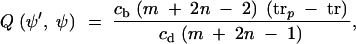where c_b and c_d are the numbers of legal demes of subtree g〈r̂, r〉 for a birth or death move, respectively.

Migration pair birth/death move:

This move operates on the topology by birth or death of two migration events. The operation is illustrated at the top of Figure 1. The birth and death operations are chosen with equal probability.

Pair death acts as follows. A tree edge 〈r̂, s〉 is chosen uniformly at random from E. If either r, s ∉ ℳ then the proposal is rejected and the MCMC update is counterincremented. Let r̂, š ∈ V, respectively denote the parent of r and child of s. Let i_r and i_š denote the deme values on 〈r̂, r〉 and 〈s, š〉, respectively. If i_r ≠ i_š, the move is rejected and the MCMC update is counterincremented. Otherwise, the candidate state is generated by replacing the edges 〈r̂, r〉, 〈r, s〉, and 〈s, š〉 in E with an edge 〈r̂, š〉. The parameters λ, μ, and Θ are unchanged.

Pair birth acts as follows. A tree edge 〈r, s〉 is chosen uniformly at random from E. Two new migration nodes are inserted at times τ₁ and τ₂, each chosen uniformly at random on t_s < τ < t_r. Suppose the deme on 〈r, s〉 was i_s. The deme on the new edge is chosen uniformly at random from 𝒟_−is. The Hastings-Green factor for the pair-birth proposal is

A3

Although acceptance rates were low (∼2%), the mixing per CPU time was good because no likelihood calculation needs to be done.

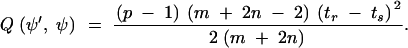
Coalescent node merge/split move:

This move operates on the topology. Migration events split or merge as they are dragged through a coalescent node. The number of migration nodes changes by one. The operation is illustrated at the bottom of Figure 1. The move proceeds as follows. A coalescent node r is chosen uniformly at random from 𝒞.

With probability one-half, a merge operation is attempted, and otherwise a split operation.

The split operator acts as follows:

Let r̂ denote the parent of r and ř₁ and ř₂ its two children. If r̂ ∉ ℳ, the move is rejected and the MCMC is counterincremented. Otherwise, let

^

r̂

denote the parent of r̂ and i_r̂ the deme label on edge , r̂. The edges , r̂ and , r are replaced by an edge , r. The deme label i_r for the new edge is set equal to i_r̂. On the child side of r, two new migration nodes s₁ and s₂ are inserted at times τ₁ and τ₂, chosen uniformly at random on t_r̂1< τ₁ < t_r and t_r̂2 < τ₂ < t_r, respectively. For a = 1, 2, edge 〈r̂, ř_a〉 is replaced by edges 〈r, s_a〉 and 〈s_a, ř_a〉 and deme value is assigned.

The merge operator acts as follows. If either ř₁, ř₂ ∉ ℳ, the move is rejected and the MCMC is counterincremented. For a = 1, 2, let

ˇ

řa

denote the child of

ˇ

řa

. If i_ř1 ≠ i_ř2, the move is likewise rejected. Otherwise, for a = 1, 2, edges ř_a, _a and 〈r, ř_a〉 are replaced by an edge r, _a. This deletes migration nodes ř₁ and ř₂. On the parent side of r, a new migration node s is inserted at a time τ chosen uniformly at random on (t_r̂, t_r). Edge 〈r̂, r〉 is replaced by edges 〈r̂, s〉 and 〈s, r〉 and deme labels i_s = i_r and are assigned.

The Hastings-Green ratio for the split operator is

The move above splits from, and merges to, a migration node on the parent edge only. It is straightforward to modify the move so that any of the three edges can assume the status that the parent edge has in the move above. Again this move has a low acceptance ratio (∼1%) but acceptance/rejections can be evaluated very rapidly.

References

- Bahlo, M., and R. C. Griffiths, 2000. Inference from gene trees in a subdivided population. Theor. Popul. Biol. 57: 79–95. [DOI] [PubMed] [Google Scholar]
- Beerli, P., and J. Felsenstein, 1999. Maximum-likelihood estimation of migration rates and effective population numbers in two populations using a coalescent approach. Genetics 152: 763–773. [DOI] [PMC free article] [PubMed] [Google Scholar]
- Beerli, P., and J. Felsenstein, 2001. Maximum likelihood estimation of a migration matrix and effective population sizes in n subpopulations by using a coalescent approach. Proc. Natl. Acad. Sci. USA 98(8): 4563–4568. [DOI] [PMC free article] [PubMed] [Google Scholar]
- Drummond, A., and A. Rodrigo, 2000. Reconstruction genealogies of serial samples under the assumption of a molecular clock using serial-sample UPGMA. Mol. Biol. Evol. 17 (12): 1807–1815. [DOI] [PubMed] [Google Scholar]
- Drummond, A. J., G. K. Nicholls, A. G. Rodrigo and W. Solomon, 2002. Estimating mutation parameters, population history and genealogy simultaneously from temporally spaced sequence data. Genetics 161: 1307–1320. [DOI] [PMC free article] [PubMed] [Google Scholar]
- Drummond, A. J., G. K. Nicholls, A. G. Rodrigo and W. Solomon, 2003a Tools for Constructing Chronologies, pp. 151–174. Springer-Verlag, Berlin, Heidelberg, Germany/New York.
- Drummond, A. J., O. G. Pybus, A. Rambaut, R. Forsberg and A. G. Rodrigo, 2003. b Measurably evolving populations. Trends Ecol. Evol. 8(9): 481–488. [Google Scholar]
- Felsenstein, J., 1981. Evolutionary trees from DNA sequences: a maximum likelihood approach. J. Mol. Evol. 17: 368–376. [DOI] [PubMed] [Google Scholar]
- Fisher, R. A., 1930 The Genetical Theory of Natural Selection. Clarendon Press, Oxford.
- Geyer, C. J., 1992. Practical Markov chain Monte Carlo. Stat. Sci. 7: 473–511. [Google Scholar]
- Green, P. J., 1995. Reversible jump Markov chain Monte Carlo computation and bayesian model determination. Biometrika 82: 711–732. [Google Scholar]
- Green, P. J., 2003 Highly Structured Stochastic Systems (http://www.oup.co.uk/isbn/0-19-851055-1).
- Hastings, W. K., 1970. Monte Carlo sampling methods using Markov chains and their applications. Biometrika 57: 97–109. [Google Scholar]
- Hudson, R. R., 1990 Gene genealogies and the coalescent process, pp. 1–44 in Oxford Surveys in Evolutionary Biology, Vol. 7. Oxford University Press, Oxford.
- Kingman, J., 1982. a The coalescent. Stoch. Proc. Appl. 13: 235–248. [Google Scholar]
- Kingman, J., 1982. b On the genealogy of large populations. J. Appl. Probab. 19A: 27–43. [Google Scholar]
- Metropolis, N., A. Rosenbluth, M. Rosenbluth, A. Teller and E. Teller, 1953. Equations of state calculations by fast computing machines. J. Chem. Phys. 21: 1087–1091. [Google Scholar]
- Nagylaki, T., 1980. The strong-migration limit in geographically structured populations. J. Math. Biol. 2: 101–114. [DOI] [PubMed] [Google Scholar]
- Nickle, D. C., M. A. Jensen, D. Shriner, S. J. Brodie, L. M. Frenkel et al., 2003. Volutionary indicators of human immunodeficiency virus type 1 reservoirs and compartments. J. Virol. 77: 5540–5546. [DOI] [PMC free article] [PubMed] [Google Scholar]
- Nielsen, R., and J. Wakeley, 2001. Distinguishing migration from isolation: Markov chain Monte Carlo approach. Genetics 158: 885–896. [DOI] [PMC free article] [PubMed] [Google Scholar]
- Notohara, M., 1990. The coalescent and the genealogical process in geographically structured population. J. Math. Biol. 29: 59–75. [DOI] [PubMed] [Google Scholar]
- Notohara, M., 1993. The strong-migration limit for the genealogical process in geographically structured populations. J. Math. Biol. 31: 115–122. [Google Scholar]
- Perelson, A. S., A. U. Neumann, M. Markowitz, J. M. Leonard and D. D. Ho, 1996. HIV-1 dynamics in vivo: virion clearance rate, infected cell life-span, and viral generation time. Science 271: 1582–1586. [DOI] [PubMed] [Google Scholar]
- Poss, M., A. G. Rodrigo, J. J. Gosink, G. H. Learn, D. de Vange Panteleef et al., 1998. Evolution of envelope sequences from the genital tract and peripheral blood of women infected with clade A human immunodeficiency virus type 1. J. Virol. 72(10): 8240–8251. [DOI] [PMC free article] [PubMed] [Google Scholar]
- Rodrigo, A. G., and J. Felsenstein, 1999 The Evolution of HIV. Johns Hopkins University Press, Baltimore.
- Rodriguez, F., J. L. Oliver, A. Marin and J. R. Medina, 1990. The general stochastic model of nucleotide substitution. J. Theor Biol. 142: 485–501. [DOI] [PubMed] [Google Scholar]
- Shankarappa, R., J. B. Margolick, S. J. Gange, A. G. Rodrigo, D. Upchurch et al., 1999. Consistant viral evolutionary changes associated with the progression of human immunodeficiency virus type 1 infection. J. Virol. 73: 10489–10502. [DOI] [PMC free article] [PubMed] [Google Scholar]
- Wang, T. H., Y. K. Donaldson, R. P. Brettle, J. E. Bell and P. Simmonds, 2001. Identification of shared populations of human immunodeficiency virus type 1 infecting microglia and tissue macrophages outside the central nervous system. J. Virol. 75(23): 11686–11699. [DOI] [PMC free article] [PubMed] [Google Scholar]
- Wong, J. K., C. Cignacio, F. Torrian, D. Havlir, N. J. Fitch et al., 1997. In vivo compartmentalization of human immunodeficiency virus: evidence from the examination of pol sequences from autopsy tissues. J. Virol. 71(3): 2059–2071. [DOI] [PMC free article] [PubMed] [Google Scholar]
- Wright, S., 1931. Evolution in Mendelian populations. Genetics 16: 97–159. [DOI] [PMC free article] [PubMed] [Google Scholar]
- Zhang, L., L. Rowe, T. He, C. Chung, J. Yu et al., 2002. Compartmentalization of surface envelope glycoprotein of human immunodeficiency virus type 1 during acute and chronic infection. J. Virol. 76(18): 9465–9473. [DOI] [PMC free article] [PubMed] [Google Scholar]